Experience-driven rate modulation is reinstated during hippocampal replay
Figures
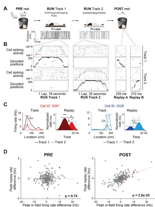
Rate coding in wake and rest.
(A) Experimental design. Each recording session, the rats rested (PRE), ran back and forth on two different linear tracks (RUN), and then rested again (POST) (left to right). An example of LFP activity in each behavioral state is displayed (RUN-theta, PRE/POST-sharp wave ripples [SWR]). Rat schematic was adapted from SciDraw.io (https://doi.org/10.5281/zenodo.3926277, https://doi.org/10.5281/zenodo.3926237, https://creativecommons.org/licenses/by/4.0). (B) Raster plots of spiking activity of cells sorted by their peak firing rate on the track (top: Track 1, n = 72 cells; bottom: Track 2, n = 57 cells), and the associated decoded positions for a single exemplar lap (first two columns) and replay event (last two columns), for each track (top: Track 1; bottom: Track 2). Because posterior probabilities are normalized across both tracks, decoded positions during behavior and replay can have substantially higher likelihood values on one track. Example from rat 3, session 2. (C) Two example neurons (highlighted in B) that changed their peak instantaneous firing rate (shaded areas, cartoon depictions of instantaneous firing rates) during two example replay events (displayed in B) in the same direction as their peak in-field firing rate difference between tracks (unshaded areas, actual ratemaps). The activity and properties of the example neurons are color coded throughout all the panels. (D) The peak in-field firing rate difference (Track 1–Track 2) significantly predicts the average peak instantaneous replay rate difference (Track 1–Track 2) in POST rest, but not PRE rest. Each data point is a neuron active on both tracks (PRE: n = 252 cells, POST: n = 272 cells).
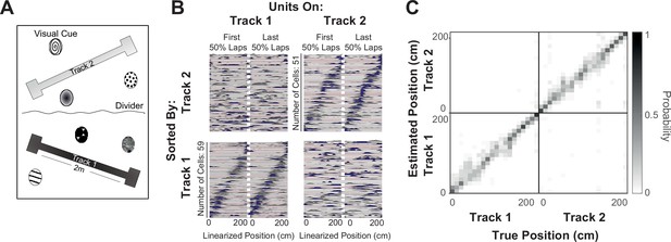
Experimental setup, remapping, and field stability.
(A) Layout of the recording room – two linear tracks, each surrounded by visual cues and visually occluded from each other. (B) Ratemaps for Track 1 (left column) and Track 2 (right column) in an example session (rat 3, session 2) computed for the first 50% of laps (left half) and last 50% of laps (right half) and sorted by the ordered position of place fields on Track 1 (bottom) and Track 2 (top). (C) Confusion matrix for decoded position (posterior probability normalized over both tracks) for an example session (rat 3, session 2). Distribution of peak posterior probabilities (y-axis) is plotted at each True position during the behavioral episode (x-axis).
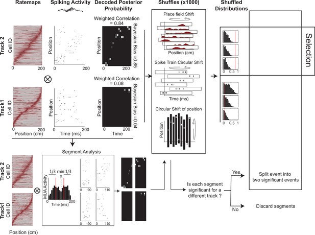
Analysis pipeline for detection of significant replay events.
Detected replay spike trains were decoded using a Bayesian framework. Each track’s ratemaps obtained during RUN were used to calculate the decoded posterior probabilities for each replay sequence (top left). In addition, all replay events were split into two shorter events based on the minimum in the multi-unit activity (MUA) during the middle third of the replay event (bottom left, segment analysis). For each replay event, weighted correlations were calculated on decoded posterior probability from both the whole replay sequence and each segment, and the three scores were compared to three different shuffles (place field shift, spike train circular shift, and circular shift of position, 1000 shuffles performed for each type). Only events with weighted correlation scores higher than 95% for every shuffle distribution (97.5% for split replay events) were considered statistically significant.
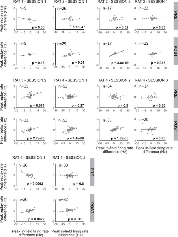
Reinstatement of rate modulation during replay for each individual session.
The peak in-field firing rate difference (Track 1–Track 2) significantly predicts the average peak instantaneous replay rate difference (Track 1–Track 2) in POST in 8 out of 10 session. In contrast, only 1 out of 10 session have a statistically significant regression in PRE. Each data point is a neuron active on both tracks. Significance and number of data points (common cells in both tracks) are indicated in each plot.
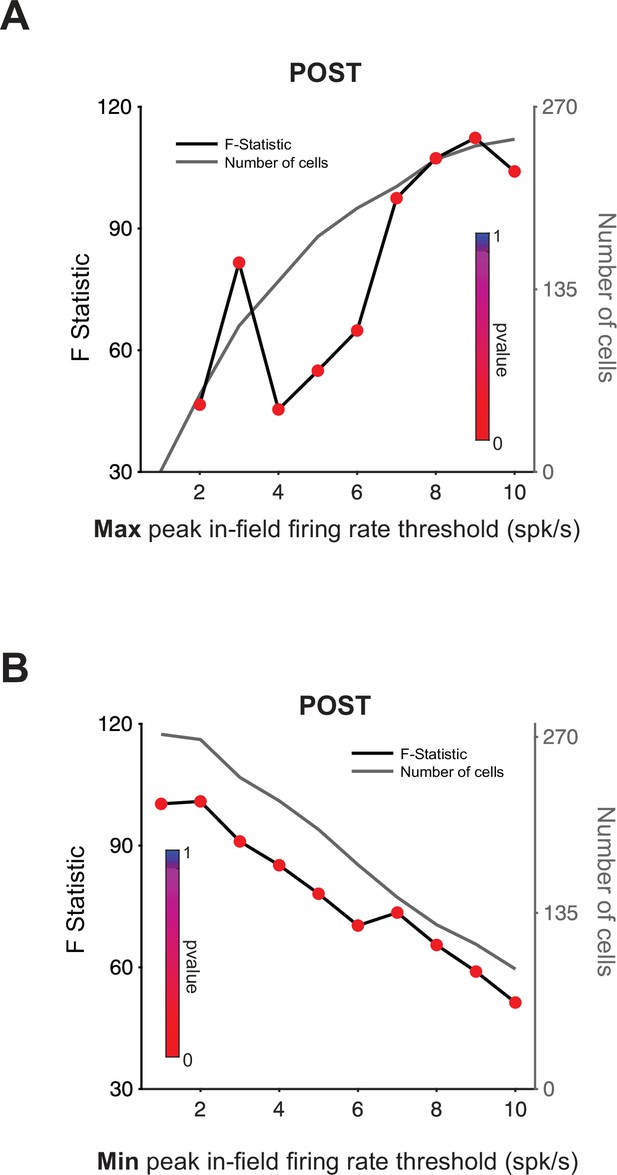
Significance of regression analysis using a stricter criterion of place cell activity.
(A) F-statistic of regression – peak in-field firing rate vs. peak replay rate (track difference) – for replay events occurring during POST, as the criterion for place cell activity (maximum peak in-field firing rate) is progressively increased from 1 Hz to 10 Hz. The first regression that only included place cells with a maximum peak in-field firing rate of 1 Hz is absent as no cells met this criterion. All the remaining regressions are statistically significant (up to and including using a threshold of 10 spk/s). The p-value of each regression is indicated by color. The number of cells used in each regression is indicated by the green line. (B) F-statistic of regression – peak in-field firing rate vs. peak replay rate (track difference) – for replay events occurring during POST, as the criterion for place cell activity (minimum peak in-field firing rate) is progressively increased from 1 Hz to 10 Hz. All regressions are statistically significant (up to and including using a threshold of 10 spk/s). The p-value of each regression is indicated by color. The number of cells used in each regression is indicated by the green line.
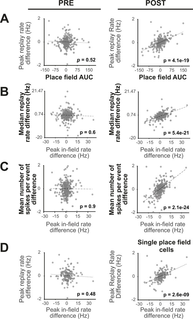
Significance of regression analysis with alternative place field and replay rate metrics, and stricter criteria for cell selection.
F-statistic of regression – peak in-field firing rate vs. peak replay rate (track difference) – for replay events occurring during PRE (left column) and POST (right column) using alternative metrics: (A) Place field area under the curve (new x-axis, PRE: n = 252 cells, POST: n = 272 cells), (B) Median replay rate (new y-axis, PRE: n = 252 cells, POST: n = 272 cells), and (C) mean number of spike per event (new y-axis, PRE: n = 252 cells, POST: n = 272 cells). And using new criteria for cell selection: (D) single place field cells (PRE: n=137 cells, POST: n = 153 cells).
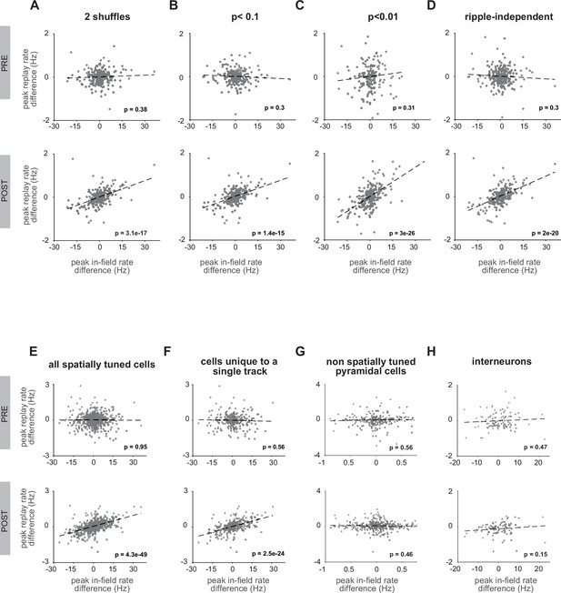
Significance of regression analysis with alternative criteria for replay detection and cell selection.
F-statistic of regression – peak in-field firing rate vs. peak replay rate (track difference) – for replay events occurring during PRE (top row) and POST (bottom row) using alternative metrics for replay detection and place cell inclusion: (A) Two shuffles (detected/candidate event ratio PRE = 18.4% 1565/8485, POST = 27.3% 3917/14326). (B) p-Value<0.1 used for replay detection (detected/candidate event ratio PRE = 21.2% 1803/8485, POST = 31.3% 4483/14326). (C) p-Value<0.01 used for replay detection (detected/candidate event ratio PRE = 2.5% 211/8485, POST = 8.3% 1195/14326). (D) No ripple power threshold for replay detection (detected/candidate event ratio PRE = 14.9% 1262/8485, POST = 22.0% 3157/14326). (E) All spatially tuned cells (PRE: n = 653 cells, POST: n = 740 cells). (F) Only place cells with place fields on a single track (PRE: n = 304 cells, POST: n = 359 cells). (G) Non-spatially tuned pyramidal cells – with a firing rate less than 1 spk/s on both tracks (PRE: n = 258 cells, POST: n = 366 cells). (H) Interneurons (PRE: n = 106 cells, POST: n = 107 cells).
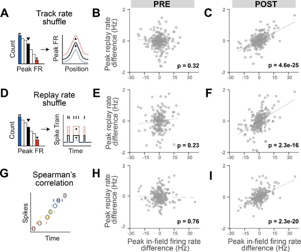
The reinstatement of rate modulation during rest replay is observed using replay detection methods insensitive to firing rate.
(A, D, G) Three methods of replay detection that are insensitive to firing rate: (A) track rate shuffle (PRE: n = 252 cells, POST: n = 271 cells), (D) replay rate shuffle (PRE: n = 186 cells, POST: n = 261 cells), (G) rank-order correlation (Spearman), where black circles indicate median spike times (PRE: n = 253 cells, POST: n = 271 cells). (A, D) Example of the original rate (right plot, in black) randomly scaled up (right plot, in red) or down (right plot, in blue), after drawing a random value from the rate distribution (left plot). (B, E, H) Regression of peak in-field firing rate vs. peak replay rate difference (Track 1–Track 2) for PRE replay events with modified detection method: (B) track rate shuffle, (E) replay rate shuffle, and (H) Spearman’s correlation. (C, F, I) Regression of peak in-field firing rate vs. peak replay rate difference (Track 1–Track 2) for POST replay events with modified detection method: (C) track rate shuffle, (F) replay rate shuffle, and (I) Spearman’s correlation. The number of cells for each analysis varies as a consequence of different sets of replay events being respectively selected and therefore included in the regressions.
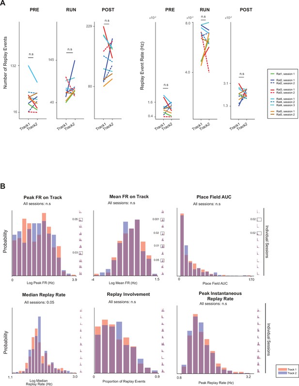
Between-track comparison of place field and replay properties.
(A) Number of replay events (left) and replay event rate (right) for each track during PRE, RUN, and POST. The differences between tracks for any of these comparisons were not statistically significant (Wilcoxon sign-rank, p>0.05, n = 10). (B) Distribution of peak firing rate on track (top left), mean firing rate on track (top center), place field area under the receiver-operating characteristic curve (AUC) (top right), median replay rate (bottom left), replay involvement (bottom center), and peak instantaneous replay rate (bottom right) for tracks 1 and 2, and for individual session distributions (inset) (Kolmogorov–Smirnov test, n.s. p>0.05).
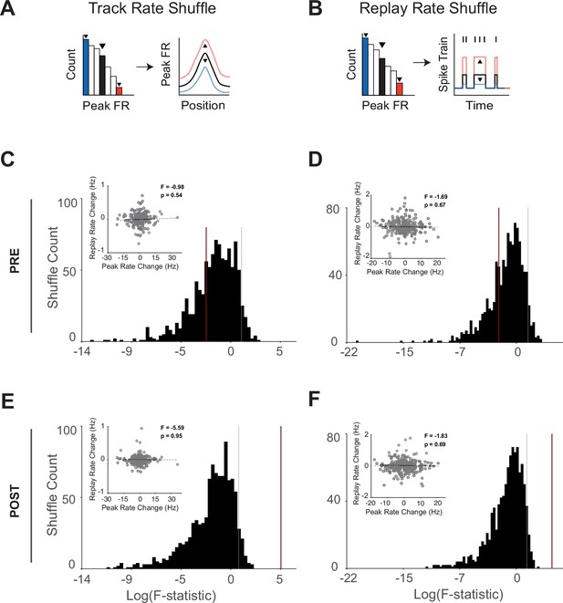
Recomputing the statistical significance of regression analysis relative to a shuffled distribution.
(A) Track rate shuffle and (B) replay rate shuffle were used to randomize the overall firing rate of place fields within a track (x-axis) and the cell’s firing rate during replay events (y-axis), respectively. An F-statistic distribution was then calculated to measure the significance of the regression. (A, B) Example of the original rate (right plot, in black) randomly scaled up (right plot, in red) or down (right plot, in blue), after drawing a random value from the rate distribution (left plot). (C–F) F-statistic distributions obtained from the shuffle (black), where dashed gray line indicates p<0.05, and red line indicates the F-statistic value of original data (main plot Figure 1D). One example of a regression plot within the shuffle distribution (inset plot). (C) PRE: track rate shuffle. (D) PRE: replay rate shuffle. (E) POST: track rate shuffle. (F) POST: replay rate shuffle.
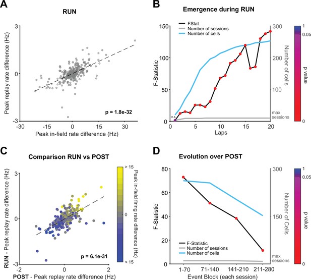
Rate modulation during replay is observed from the beginning of RUN and continues throughout the entire RUN and POST epochs.
(A) Regression of peak in-field firing rates against peak replay rates (track differences) for all local RUN replay events. (B) Lap by lap emergence of rate modulation for RUN local replay events. F-statistic of regression – peak in-field firing rate vs. peak replay rate (track difference) – for replay events occurring both prior to and including the specified lap. The p-value of each regression is indicated by color. The number of cells and number of data sessions contributing in each regression are indicated with the cyan and gray line, respectively. (C) Peak replay rate difference for replay events (RUN vs. POST), color coded by peak in-field rate differences between tracks. (D) Temporal dynamics of rate modulation during POST. The regression’s F-statistic (y-axis) and the corresponding p-value (marker color), analyzed in non-overlapping blocks of 70 consecutive replay events (per session). The number of cells and number of data sessions contributing in each regression are indicated with the cyan and gray line, respectively.
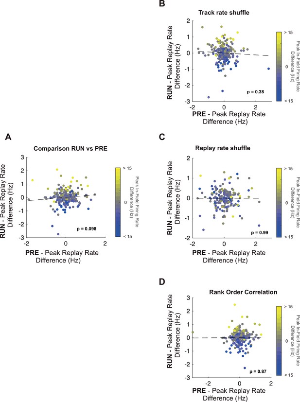
Between track differences in replay rate during PRE is not predictive of replay rate differences observed during RUN local replay events.
(A) Peak replay rate difference for replay events (RUN vs. PRE), color coded by peak in-field rate differences. A linear regression was not statistically significant (p=0.1) using our main replay event detection method, and we did not observe a significant regression (p>0.05) for any of the three alternative methods that control for rate biases in selective significant replay events. (B) Track rate shuffle, (C) replay rate shuffle, and (D) rank-order (Spearman) correlation.
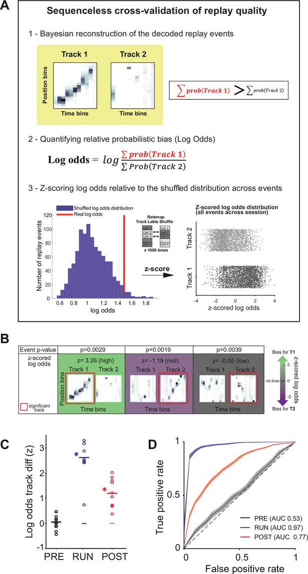
Sequenceless decoding to cross-validate replay events.
(A) Description of a sequenceless decoding based method for cross-validating replay events originally detected based on sequenceness. (1) Events are decoded, and the posterior probabilities summed across each track, (2) the log odds ratio is calculated, and (3) this ratio is z-scored using a log odds distribution, based on place fields with shuffled track identity. (B) Example of three replay events scored as significant based on their sequenceness (i.e., order of cell activation) (top row ‘Event p-value’), while presenting different posterior probability distributions across the two tracks (bottom row ‘z-scored log odds’). From left to right, examples of replay events with high, medium, and low z-scored log odds, respectively. (C) The decoding performance for context (Track 1 or Track 2) using the mean z-scored log odds difference between tracks for replay during PRE (black), RUN (blue), and POST (red). Each data point is the mean of an individual session, while the horizontal line indicates the mean across all sessions (*p<0.05, one-tailed rank-sum test). The filled box indicates the SD from the replay track identity shuffles. (D) Receiver-operative characteristic (ROC) curves of Track 1/Track 2 binary discrimination for replay events during PRE, RUN, and POST. The dashed line along the diagonal indicates chance performance (area under the ROC curve [AUC] = 0.5). The shaded region indicates the bootstrapped SE of the ROC curves.
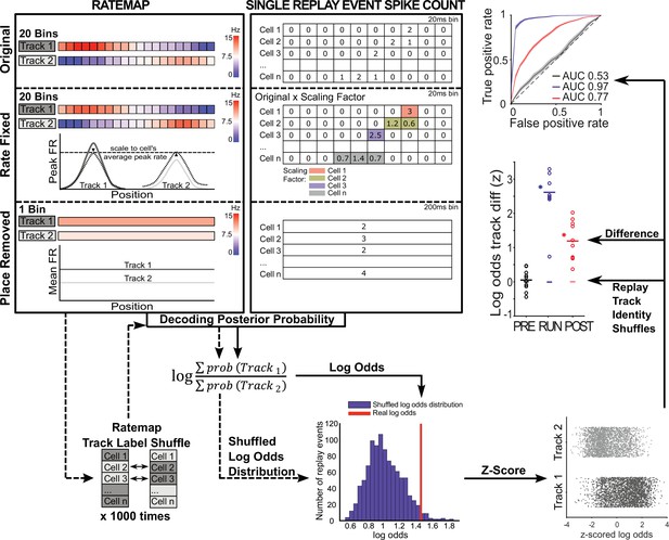
Schematic of modified Bayesian decoding framework.
The concatenated Track 1 and Track 2 ratemap (top first column) and spike counts during each replay event (top second column) are used for Bayesian decoding. This produces a posterior probabilistic distribution for each replay event, which is normalized across all position bins from both tracks to sum to 1 (original, top row). Then, the relative probabilistic bias between Track 1 and Track 2 (log odds) is computed. As control conditions, the original ratemap and replay spike counts are selectively modified such that only place information (rate fixed manipulation, second row) or rate information (place removed manipulation, third row) is available for Bayesian decoding. For rate fixed manipulation, rate information is fixed by (1) rescaling each cell’s peak in-field firing rate to the mean value across both tracks, and (2) rescaling its spike count during each replay event to the average firing rate across all replay events. For place removed manipulation, the place and sequence information is removed by decoding using only a single position bin covering the entire track (when the animal’s moving speed is above 5 cm/s) and a single time bin spanning the entire replay event. For all conditions, the manipulated replay events are next decoded using the original decoding pipeline, including a Track 1 and Track 2 ratemap track label shuffle, obtained by randomly permuting each cell’s Track 1 and Track 2 ratemaps 1000 times for each replay event (bottom left). The permutation is done by either keeping a cell’s ratemap unaltered or performing a between track swap. The z-scored log odds for each replay event is obtained by comparing the raw log odds relative to the shuffled log odds distribution. For each behavioral epoch (i.e., PRE, RUN, and POST), Track 1 and Track 2 z-scored log odds distributions are obtained by classifying each replay event according to the track identity determined by the sequenceness of the replay (bottom right). The track discrimination performance is quantified using two measurements. The first method quantifies binary discriminability using receiver-operative characteristic curve (ROC curve). In brief, the ROC curve is constructed by plotting the true-positive rate against false-positive rates obtained by shifting discrimination threshold across the two z-scored log odds distributions. The area under the ROC curve (AUC) would thereby indicate the performance of binary discriminability where AUC = 1 indicates perfect discrimination and AUC = 0.5 indicates chance-level discrimination (right, top plot). The second method quantifies the mean difference between Track 1 and Track 2 z-scored log odds distributions. The mean z-scored log odds track difference for each behavioral epoch is obtained by taking the average of the z-scored log odds track difference across all replay events within each session and then across all 10 sessions. The statistical significance for this measurement is quantified using one-tailed rank-sum test in which the mean z-scored log odds track difference from 10 sessions are compared to the shuffled version of the log odds track differences distribution where the replay events from each session were resampled with replacement 1000 times and their track identities were assigned randomly (referred to as replay track identity shuffle) (right, bottom plot).
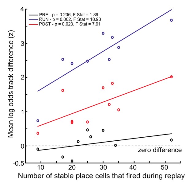
The relationship between the number of stable place cells that participated in replay and the mean log odds track difference during PRE (black), RUN (blue), and POST (red).
Each dot represents the mean value of an individual session. The horizontal dashed line indicates zero track difference. A linear regression was considered statistically significant when p<0.05.
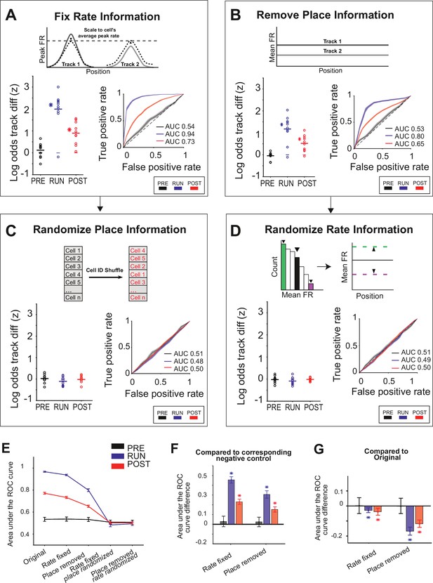
Either place or rate representations can be used to classify the replayed context.
(A–D) The decoding performance for context (Track 1 or Track 2) for each manipulation, restricting the information (rate and/or place) available to the decoder. (Main plots) Mean z-scored log odds difference between tracks for replay during PRE (black), RUN (blue), and POST (red). Each data point is the mean of an individual session, while the horizontal line indicates the mean across all sessions (*p<0.05, one-tailed rank-sum test). The filled box indicates the SD from the replay track identity shuffles. (Insets) Receiver-operative characteristic (ROC) curves of Track 1/Track 2 binary discrimination for replay events during PRE, RUN, and POST. The dashed line along the diagonal indicates chance performance (area under the ROC curve [AUC] = 0.5). The shaded region indicates the bootstrapped SE of the ROC curves. (A) Rate fixed manipulation (only place information available), (B) place removed manipulation (only rate information available), (C) rate fixed manipulation with place information additionally randomized (no rate or place information available), and (D) place removed manipulation with rate information additionally randomized (no rate or place information available). (E) Summary of mean and SEM AUC under each manipulation condition, for PRE, RUN, and POST. (F) Mean AUC difference between each manipulation and the corresponding negative control. (G) Mean AUC difference between original and rate fixed and place removed manipulation. For (F, G), asterisks (*) indicate where the 95% confidence interval of the bootstrapped AUC difference distribution does not overlap with 0 (Table 3A and B). Similar results were obtained using an alternative approach (DeLong method) for measuring significance (Table 3C and D; see ‘Methods’).
Tables
Overview of behavior, number of recorded cells, and decoding accuracy for all sessions and rats.
| Time resting(min) | Cells | Decoding quality (%) | |||||||
|---|---|---|---|---|---|---|---|---|---|
| Session | Track | Number of laps | PRE | POST | Cells used for replay analysis | Common to T1 and T2 (stable/non-stable) | Stable cells included in regression analysis | Classification accuracy | Local decoding accuracy |
| Rat 1, session 1 | 1 | 10 | 83 | 155 | 27 | 10 (9/1) | 9 | 86 | 58 |
| Rat 1, session 1 | 2 | 12 | 83 | 155 | 27 | 10 (9/1) | 9 | 93 | 66 |
| Rat 2, session 1 | 1 | 15 | 59 | 125 | 70 | 41 (29/12) | 29 | 97 | 86 |
| Rat 2, session 1 | 2 | 59 | 59 | 125 | 63 | 41 (29/12) | 29 | 93 | 89 |
| Rat 2, session 2 | 1 | 22 | 54 | 104 | 49 | 28 (17/11) | 17 | 92 | 82 |
| Rat 2, session 2 | 2 | 33 | 54 | 104 | 43 | 28 (17/11) | 17 | 90 | 79 |
| Rat 3, session 1 | 1 | 34 | 49 | 123 | 59 | 33 (25/8) | 25 | 94 | 85 |
| Rat 3, session 1 | 2 | 27 | 49 | 123 | 51 | 33 (25/8) | 25 | 94 | 80 |
| Rat 3, session 2 | 1 | 36 | 69 | 137 | 72 | 44 (33/11) | 33 | 94 | 85 |
| Rat 3, session 2 | 2 | 38 | 69 | 137 | 57 | 44 (33/11) | 33 | 97 | 86 |
| Rat 4, session 1 | 1 | 19 | 103 | 129 | 87 | 66 (52/14) | 52 | 94 | 80 |
| Rat 4, session 1 | 2 | 10 | 103 | 129 | 80 | 66 (52/14) | 52 | 94 | 85 |
| Rat 4, session 2 | 1 | 13 | 98 | 125 | 63 | 44 (35/9) | 35 | 88 | 78 |
| Rat 4, session 2 | 2 | 11 | 98 | 125 | 52 | 44 (35/9) | 35 | 97 | 82 |
| Rat 4, session 3 | 1 | 30 | 72 | 76 | 42 | 30 (20/10) | 20 | 91 | 81 |
| Rat 4, session 3 | 2 | 20 | 72 | 76 | 44 | 30 (20/10) | 20 | 97 | 82 |
| Rat 5, session 1 | 1 | 13 | 91 | 76 | 50 | 31 (20/11) | 20 | 97 | 85 |
| Rat 5, session 1 | 2 | 11 | 91 | 76 | 57 | 31 (20/11) | 20 | 90 | 89 |
| Rat 5, session 2 | 1 | 13 | 72 | 86 | 70 | 47 (32/15) | 32 | 94 | 88 |
| Rat 5, session 2 | 2 | 19 | 72 | 86 | 66 | 47 (32/15) | 32 | 94 | 87 |
Summary statistics of the z-scored log odds difference per session and across sessions for PRE, RUN, and POST.
| Original | Rate fixed | Place removed | Rate fixed, place randomized | Place removed, rate randomized | ||||||||||||
|---|---|---|---|---|---|---|---|---|---|---|---|---|---|---|---|---|
| Session | Mean | SE | p-Value | Mean | SE | p-Value | Mean | SE | p-Value | Mean | SE | p- Value | Mean | SE | p- Value | |
| PRE | Rat1 Session1 | –0.09 | 0.32 | 0.02 | –0.03 | –0.30 | ||||||||||
| Rat2 Session1 | 0.27 | 0.38 | 0.02 | 0.04 | 0.00 | |||||||||||
| Rat Session2 | –0.32 | –0.51 | –0.34 | 0.31 | 0.03 | |||||||||||
| Rat3 Session1 | 0.13 | –0.21 | 0.06 | –0.37 | 0.05 | |||||||||||
| Rat3 Session2 | 0.47 | 0.65 | 0.00 | –0.05 | 0.17 | |||||||||||
| Rat4 Session1 | 0.17 | 0.22 | 0.06 | 0.12 | –0.08 | |||||||||||
| Rat4 Session2 | 0.02 | 0.27 | –0.05 | 0.06 | 0.23 | |||||||||||
| Rat4 Session3 | –0.13 | –0.01 | –0.04 | –0.19 | –0.18 | |||||||||||
| Rat5 Session1 | –0.44 | –0.17 | –0.35 | 0.23 | –0.04 | |||||||||||
| Rat5 Session2 | 0.46 | 0.26 | 0.18 | 0.13 | –0.11 | |||||||||||
| Mean | 0.05 | 0.10 | 0.24 | 0.12 | 0.11 | 0.21 | –0.04 | 0.05 | 0.43 | 0.03 | 0.06 | 0.24 | –0.02 | 0.05 | 0.69 | |
| RUN | Rat1 Session1 | 0.74 | –0.19 | –0.11 | –0.34 | 0.05 | ||||||||||
| Rat2 Session1 | 3.29 | 2.36 | 1.47 | –0.05 | –0.07 | |||||||||||
| Rat2 Session2 | 2.53 | 2.31 | 1.22 | –0.29 | –0.21 | |||||||||||
| Rat3 Session1 | 2.48 | 2.42 | 0.35 | –0.35 | –0.05 | |||||||||||
| Rat3 Session2 | 3.17 | 2.23 | 1.52 | –0.18 | 0.06 | |||||||||||
| Rat4 Session1 | 3.67 | 3.00 | 2.04 | 0.18 | 0.23 | |||||||||||
| Rat4 Session2 | 2.88 | 2.02 | 1.40 | –0.31 | –0.18 | |||||||||||
| Rat4 Session3 | 2.45 | 2.10 | 1.11 | 0.03 | –0.32 | |||||||||||
| Rat5 Session1 | 2.41 | 1.89 | 1.07 | 0.17 | –0.25 | |||||||||||
| Rat5 Session2 | 2.53 | 1.80 | 1.67 | 0.10 | –0.14 | |||||||||||
| Mean | 2.61 | 0.25 | 9.13 × 10⁻⁵ | 1.99 | 0.26 | 1.41 × 10⁻³ | 1.17 | 0.20 | 1.41 × 10⁻³ | –0.11 | 0.07 | 0.79 | –0.09 | 0.05 | 0.94 | |
| POST | Rat1 Session1 | 0.37 | 0.06 | –0.06 | –0.05 | –0.09 | ||||||||||
| Rat2 Session1 | 1.70 | 1.11 | 0.59 | 0.21 | –0.03 | |||||||||||
| Rat2 Session2 | 1.62 | 1.40 | 0.80 | –0.36 | 0.08 | |||||||||||
| Rat3 Session1 | 0.70 | 0.78 | 0.18 | –0.13 | –0.07 | |||||||||||
| Rat3 Session2 | 1.83 | 1.57 | 0.87 | 0.05 | –0.13 | |||||||||||
| Rat4 Session1 | 2.02 | 1.51 | 1.12 | 0.09 | –0.01 | |||||||||||
| Rat4 Session2 | 1.06 | 0.80 | 0.49 | –0.04 | 0.07 | |||||||||||
| Rat4 Session3 | 0.72 | 0.34 | 0.26 | 0.17 | –0.09 | |||||||||||
| Rat5 Session1 | 0.68 | 0.42 | 0.21 | –0.05 | 0.10 | |||||||||||
| Rat5 Session2 | 1.21 | 0.97 | 0.73 | –0.05 | 0.01 | |||||||||||
| Mean | 1.19 | 0.18 | 9.13 × 10⁻⁵ | 0.90 | 0.16 | 9.13 × 10⁻⁵ | 0.52 | 0.12 | 1.41 × 10⁻³ | –0.02 | 0.05 | 0.79 | –0.02 | 0.03 | 0.79 | |
Summary statistics for the binary discriminability of a replay event’s track identity using receiver-operative characteristic (ROC) curves under the original and manipulated conditions.
(A) Summary statistics of the 95% confidence interval for the area under the receiver-operative characteristic (AUC) curve difference between the original and the manipulated conditions. (B) The manipulated conditions and their respective negative controls. (C) Summary statistics of the DeLong test comparing the ROC curves between the original and the manipulated condition. (D) Summary statistics of the DeLong Test comparing the ROC curves between the manipulated conditions and their respective negative controls.
| A | Vs. original 95% confidence interval | |||
|---|---|---|---|---|
| PRE | RUN | POST | ||
| Original vs. rate fixed | Mean AUC Diff | 0.002 | –0.03 | –0.04 |
| SEM AUC Diff | 0.03 | 0.01 | 0.01 | |
| Lower CI | –0.05 | –0.05 | –0.06 | |
| Upper CI | 0.06 | –0.02 | –0.02 | |
| Original vs. place removed | Mean AUC Diff | –0.002 | –0.17 | –0.12 |
| SEM AUC Diff | 0.03 | 0.01 | 0.01 | |
| Lower CI | –0.06 | –0.20 | –0.14 | |
| Upper CI | 0.05 | –0.14 | –0.09 | |
| B | Vs. negative control 95% confidence interval | |||
| PRE | RUN | POST | ||
| Rate fixed vs. rate fixed + place randomized | Mean AUC Diff | 0.03 | 0.46 | 0.23 |
| SEM AUC Diff | 0.03 | 0.02 | 0.01 | |
| Lower CI | –0.03 | 0.42 | 0.20 | |
| Upper CI | 0.08 | 0.49 | 0.26 | |
| Place removed vs. place removed + rate randomized | Mean AUC Diff | 0.03 | 0.31 | 0.15 |
| SEM AUC Diff | 0.03 | 0.02 | 0.01 | |
| Lower CI | –0.02 | 0.27 | 0.13 | |
| Upper CI | 0.08 | 0.34 | 0.18 | |
| C | DeLong test vs. original (significance = 0.05) | |||
| Original vs. rate fixed | Original vs. place removed | |||
| PRE | 0.89 | 0.95 | ||
| RUN | 1.84 × 10⁻⁶ | 6.48 × 10–52 | ||
| POST | 1.37 × 10⁻⁵ | 3.42 × 10⁻³⁵ | ||
| D | DeLong test vs. negative control (significance = 0.05) | |||
| Rate fixed vs. rate fixed + place randomized | Place removed vs. place removed + rate randomized | |||
| PRE | 0.24 | 0.31 | ||
| RUN | 1.94 × 10–163 | 1,00 × 10–55 | ||
| POST | 3.00 × 10–64 | 1.82 × 10⁻²⁸ | ||
-
Bold values statistically significant from zero.
Summary statistics for the z-scored log odds difference from 10 negative control simulations for PRE.
The negative control manipulation used for main result was selected (indicated in bold) based on the median difference value out of 10 simulations.
| Rate fixed place randomized | Place removed rate randomized | |||||
|---|---|---|---|---|---|---|
| Mean difference | SE | p-Value | Mean difference | SE | p-Value | |
| Sim 1 | 0.18 | 0.06 | 0.002 | 0.18 | 0.06 | 0.002 |
| Sim 2 | –0.08 | 0.12 | 0.79 | 0.01 | 0.05 | 0.79 |
| Sim 3 | –0.01 | 0.12 | 0.52 | –0.03 | 0.06 | 0.79 |
| Sim 4 | 0.05 | 0.06 | 0.79 | –0.14 | 0.07 | 0.99 |
| Sim 5 | –0.03 | 0.04 | 0.52 | –0.02 | 0.05 | 0.57 |
| Sim 6 | 0.03 | 0.09 | 0.52 | –0.08 | 0.09 | 0.76 |
| Sim 7 | –0.02 | 0.13 | 0.52 | –0.03 | 0.05 | 0.48 |
| Sim 8 | 0.03 | 0.06 | 0.24 | –0.02 | 0.05 | 0.63 |
| Sim 9 | 0.08 | 0.11 | 0.06 | 0.01 | 0.05 | 0.052 |
| Sim 10 | –0.03 | 0.09 | 0.52 | –0.03 | 0.05 | 0.26 |


