Large-scale analysis and computer modeling reveal hidden regularities behind variability of cell division patterns in Arabidopsis thaliana embryogenesis
- Université Paris-Saclay, INRAE, AgroParisTech, Institut Jean-Pierre Bourgin, France
- Université Paris-Saclay, INRAE, MaIAGE, France
Figures
Figure 1
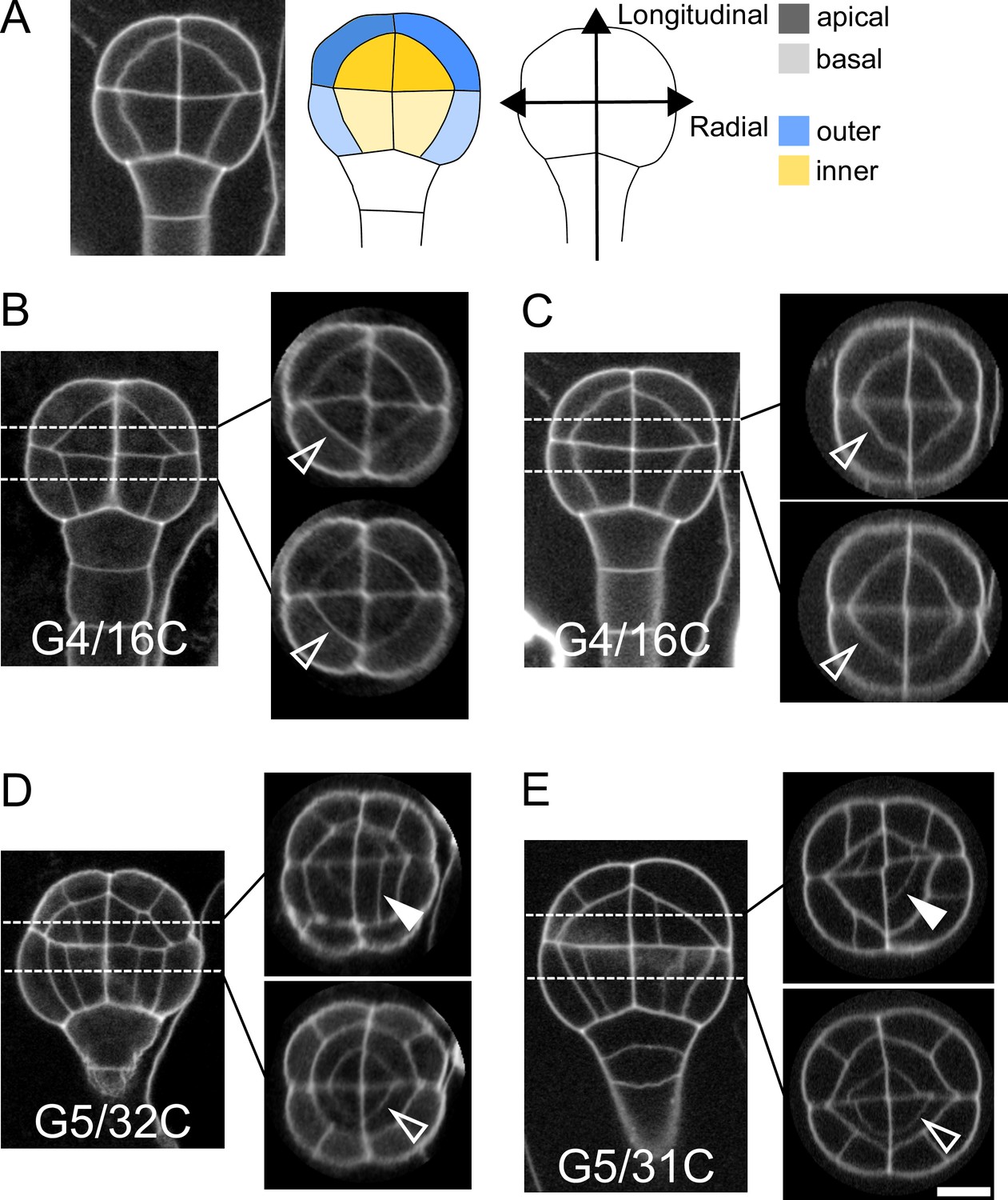
Variability within and between embryos in cell shapes and cell arrangements.
(A) The four embryo domains defined by longitudinal and radial axes at stage 16C (longitudinal view): apical/basal × outer/inner. (BC) Invariant patterns in embryos up to generation 4 (16C). (DE) Starting from generation 5, embryos show variable cell shapes and cell patterns in the apical domains, both between individuals and between quarters in a given individual. Patterns in the basal domains show little or no variability. Some of the new interfaces at G4 (BC) and at G5 (DE) are labeled using arrow heads (Empty: invariant patterns; Filled: variable patterns). Scale bar: 10 µm.
Figure 2
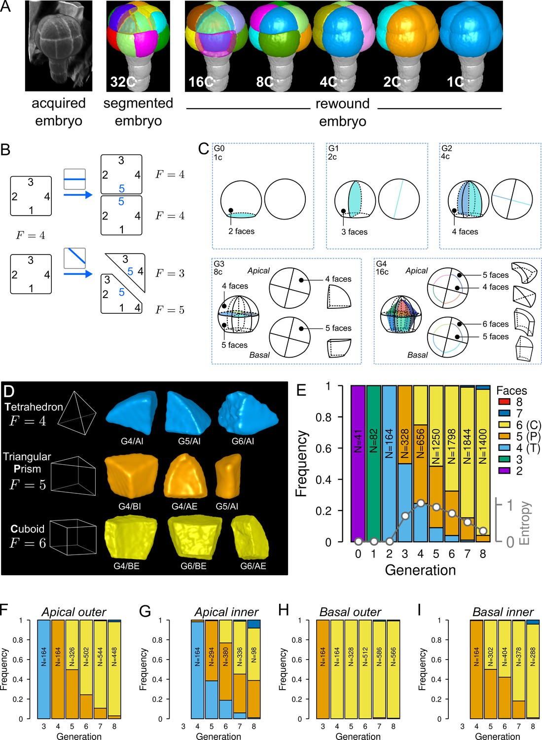
Cell shape diversity in Arabidopsis thaliana early embryogenesis.
(A) Summary of 3D image analysis pipeline: 3D cell segmentation of confocal image stacks and cell lineage reconstruction by recursive merging of daughter cells. At 32C and 16C stages, some cells are shown transparent to visualize inner cells. (B) Classification of cell shapes based on the number of division interfaces. The scheme illustrates how the number of faces may change during a division. In both examples, a cell with initially four faces divides. The number of faces in daughter cells depends on the positioning of the new interface and of whether all original faces are represented in the daughter cells. (C) Shape classification during the first four generations. (D) Samples of the three main classes of cell shapes observed during the late four generations. (E) Proportions of shape classes over the whole embryo during the first eight generations. C: Cuboid; P: Prism; T: Tetrahedron. Grey plot: entropy of the distribution among the different shape classes. (F–I) Same as (E) over the outer apical (F), the inner apical (G), the outer basal (H), and the inner basal (I) domain. N: number of observed and reconstructed cells.
-
Figure 2—source data 1
Cell shape measurements.
- https://cdn.elifesciences.org/articles/79224/elife-79224-fig2-data1-v1.zip
Figure 3 with 4 supplements
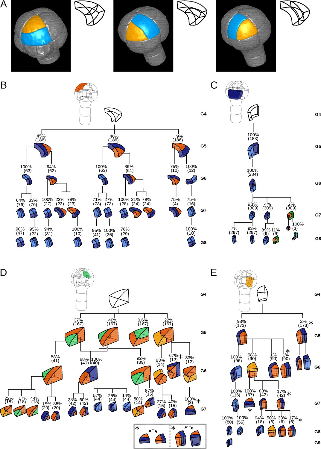
Reconstructed division patterns and cell lineages in the four embryo domains.
(A) Classification of cell division patterns (illustration in the apical outer domain) based on mother and daughter cell shapes and on the absolute orientation of division planes within the embryo. (BCDE) Lineage trees in the apical outer (B), basal outer (C), apical inner (D) and basal inner (E) domains. Each tree shows the observed combinations of cell divisions as a function of cell shapes and of generations. At each generation, frequencies were computed based on both embryos observed at this generation and later embryos that had been reconstructed at this generation by recursively merging sister cells. Numbers in parentheses are the total numbers of cases over which the percentages were calculated. Exceptionally rare division patterns are omitted in (B) and (D) for the sake of clarity; complete versions are given in Figure 3—figure supplement 1 and Figure 3—figure supplement 2. Asterisks correspond to symmetrical alternatives that were not distinguished in these trees.
Figure 3—figure supplement 1

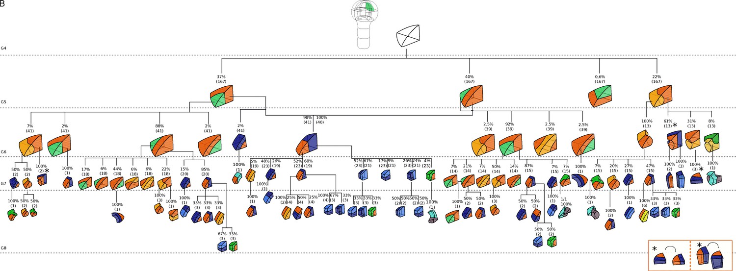
Complete reconstructed cell lineages in the apical outer domain.
Frequencies were computed based on observed patterns and patterns reconstructed at intermediate generations when rewinding lineages back to 16C stage from observed configurations. Numbers in parentheses are the total number of cases over which the percentages were calculated. Asterisks correspond to symmetrical alternatives that were not distinguished.
Figure 3—figure supplement 2
Complete reconstructed cell lineages in the apical inner domain.
Frequencies were computed based on observed patterns and patterns reconstructed at intermediate generations when rewinding lineages back to 16C stage from observed configurations. Numbers in parentheses are the total number of cases over which the percentages were calculated. Asterisks correspond to symmetrical alternatives that were not distinguished.
Figure 3—figure supplement 3
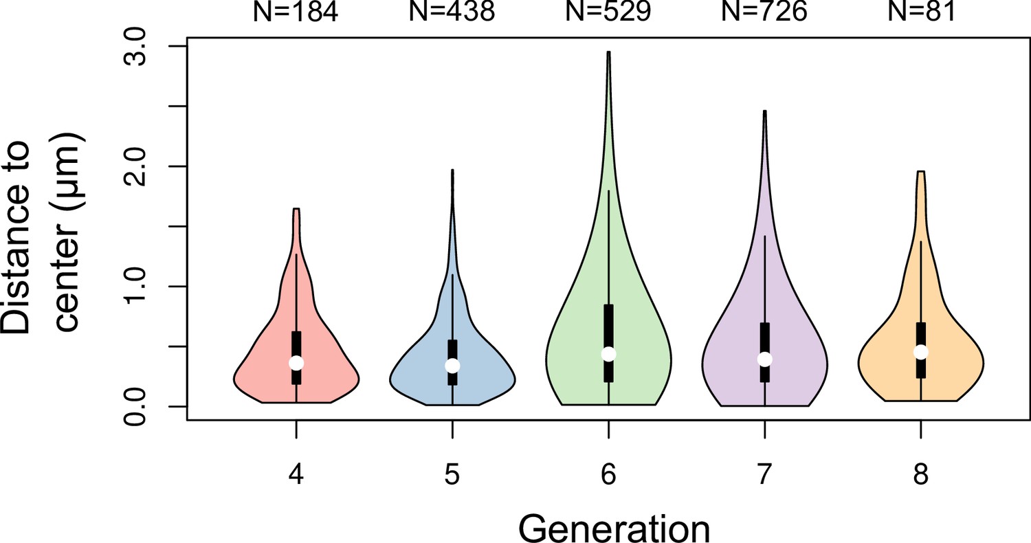
Distance between cell division plane and cell center at different generations in Arabidopsis thaliana embryos.
Distance was measured in mother cells reconstructed from identified sister cells at the immediately following generation.
Figure 3—figure supplement 4
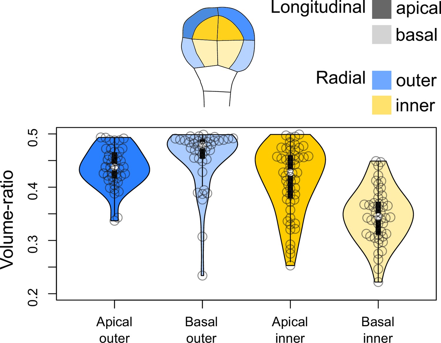
Volume-ratio of cell divisions at the G4-G5 transition in the four embryo domains (shown at G4 above the graph).
Volume-ratio of each division was computed as the ratio of cellular volumes between the smallest daughter cell and the mother cell.
Figure 4
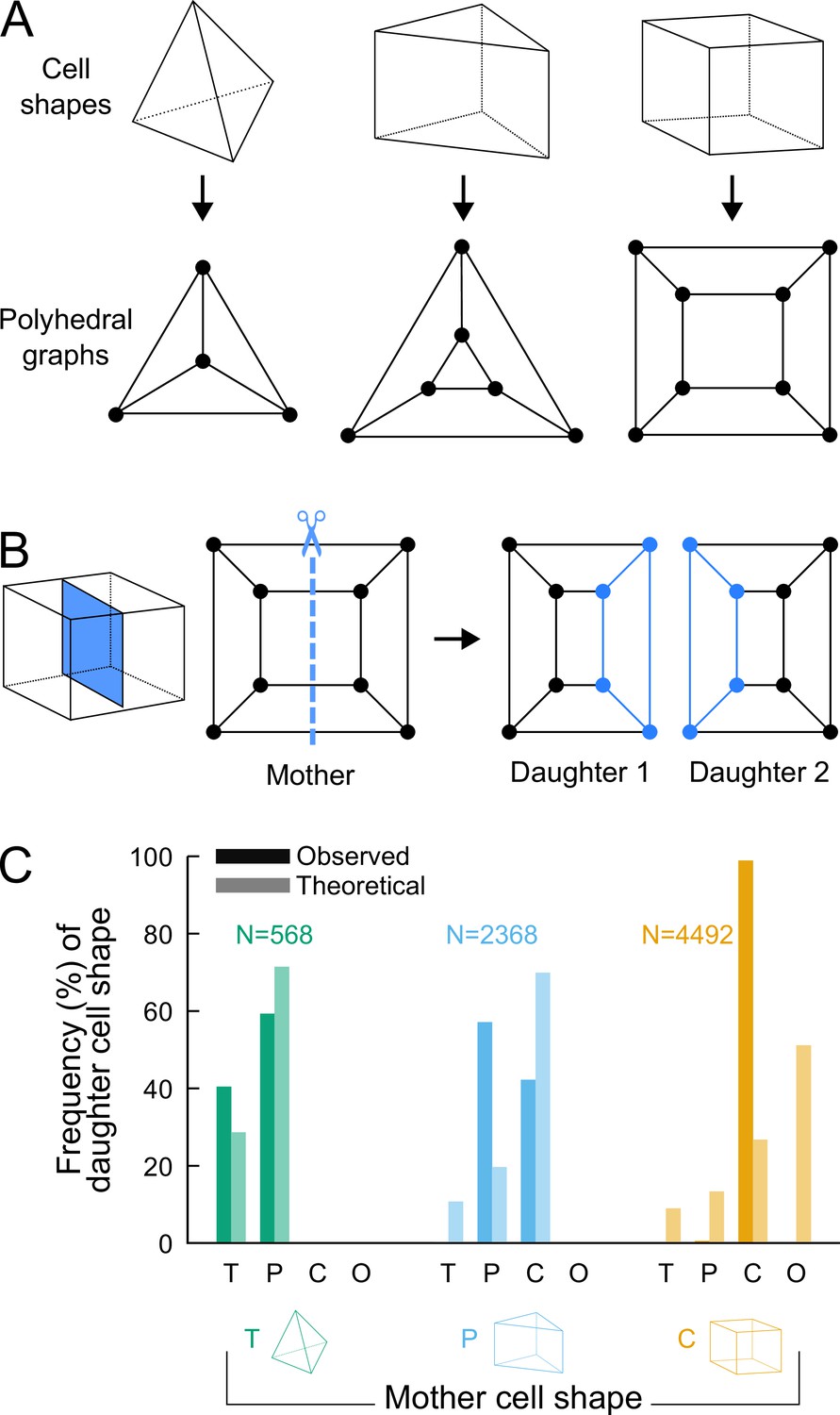
Analyzing cell divisions as graph cuts on polyhedral graphs.
(A) The three main cell shapes and their corresponding polyhedral graphs shown as Schlegel diagrams. Dots in the graphs correspond to cell vertices and lines correspond to cell edges. (B) Cell division as graph cuts: illustration with the division of a cuboid shape. The division shown on the left corresponds to the removal of four edges in the mother cell graph (edges intersected by the dotted line). New vertices and edges added in the graphs of the two resulting daughter cells are shown in blue. (C) Observed and theoretical frequencies of daughter cell shapes during the division of each cell shape. Theoretical predictions were obtained under random graph cuts. T: tetrahedron; P: triangular prism; C: cuboid; O: others.
-
Figure 4—source data 1
Theoretical and observed frequencies of daughter cell shapes.
- https://cdn.elifesciences.org/articles/79224/elife-79224-fig4-data1-v1.txt
Figure 5 with 1 supplement
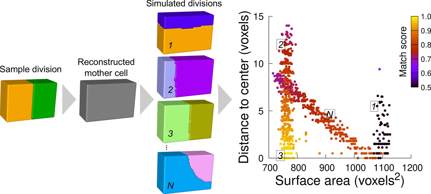
Computational strategy to analyze cell divisions: illustration with a synthetic example (symmetrical vertical division of a cuboid).
Starting from a sample division, the mother cell is reconstructed and a large number of divisions at various volume-ratios is simulated. The distance from the cell center and the surface area of the simulated planes are computed. A match score, quantifying the correspondence with the sample division, is computed for each simulated division and represented in pseudo-color. In the present case, the graph shows several families of simulated planes. The location at the bottom left of the distribution of the simulations closest to the sample pattern shows that this division corresponds the minimum plane area among the solutions that pass through the cell center.
Figure 5—figure supplement 1
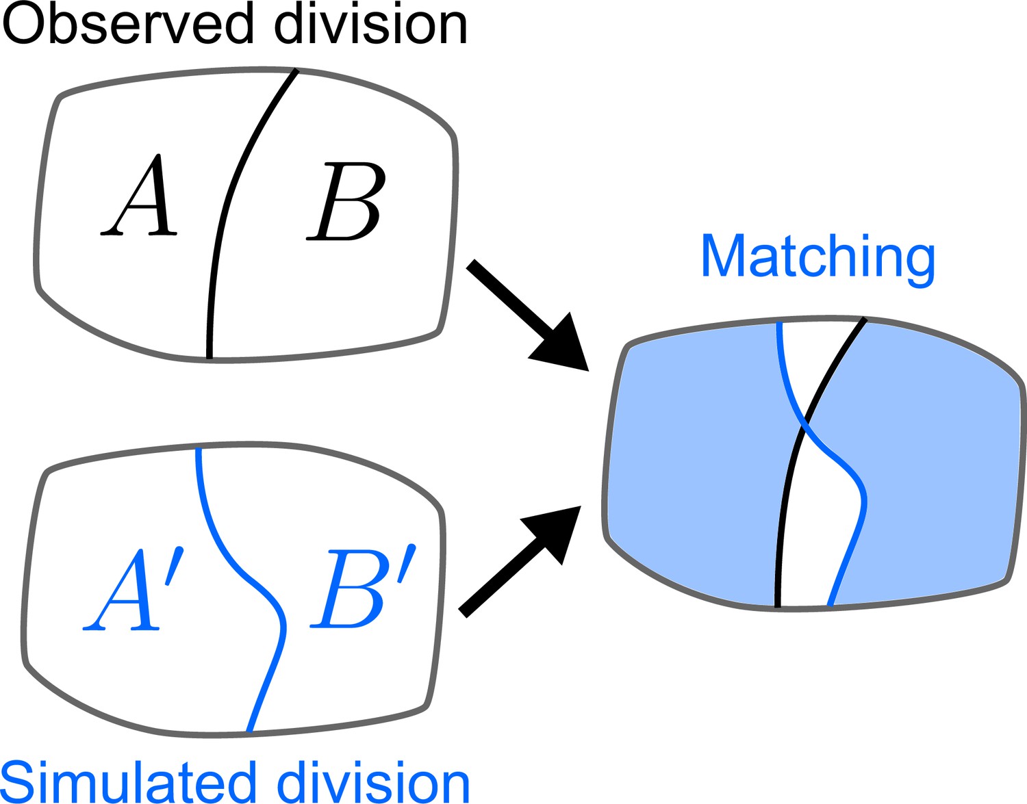
Quantifying the similarity between observed and simulated cell divisions.
The matching score is computed based on the maximum overlap between observed and daughter cells.
Figure 6 with 8 supplements
Modeling division patterns at G5 in outer cells based on geometrical features.
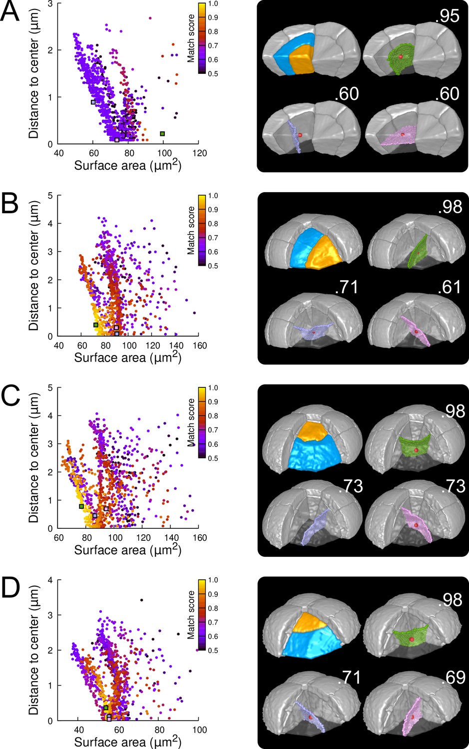
(A) Left: distribution plot of simulation results in a basal outer cell (N=1000). Simulated planes are positioned based on their surface area and distance to the mother cell center. The dot color indicates the match score between simulated and observed planes. Right: observed daughter cells (Blue and Orange); three simulated planes are shown in the reconstructed mother cell (Transparent). Green: simulation matching best with observed pattern. Lavender and Pink: simulations with alternative orientations. Numbers show the corresponding match scores. Red dot: mother cell center. In the dot plot (Left), the positions of the three simulated planes are shown as squares with the same colors. (BCD) Same as (A) for three apical outer cells that divided along the three main orientations of division.
Figure 6—figure supplement 1
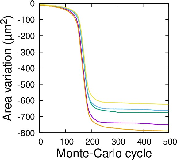
Convergence of the 3D computational model of cell division: cumulative variation of division plane area as a function of Monte Carlo cycle.
Five independent runs are illustrated. The model was run on the mother cell shown Figure 6A.
Figure 6—figure supplement 2
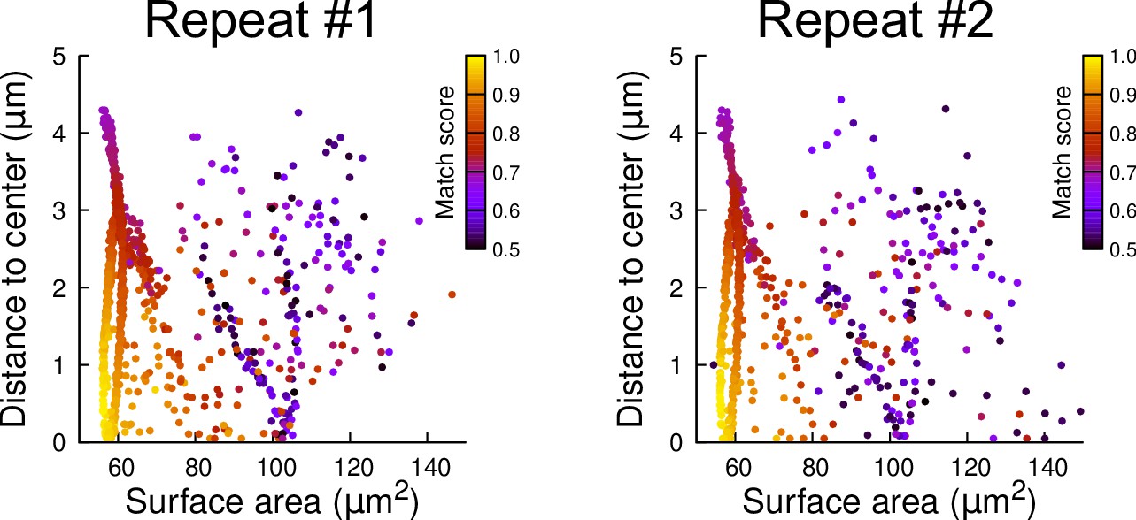
Reproducibility of simulation results: distribution plots of two independent batches of 1000 simulation runs each.
The simulations were run in a basal outer mother cell reconstructed at G4. Each simulated division is represented as a point. The color code indicates the match score between simulated and observed planes.
Figure 6—figure supplement 3

Robustness of simulation results to mother cell segmentation.
A basal outer mother cell was reconstructed at G4. Simulations were run in its raw 3D binary mask (No opening) or in its mask filtered with a mathematical morphological opening with radius R=1, 2, or 3 voxels. Each simulated division is represented as a point (1000 simulations were run in each case). The color code indicates the match score between simulated and observed planes.
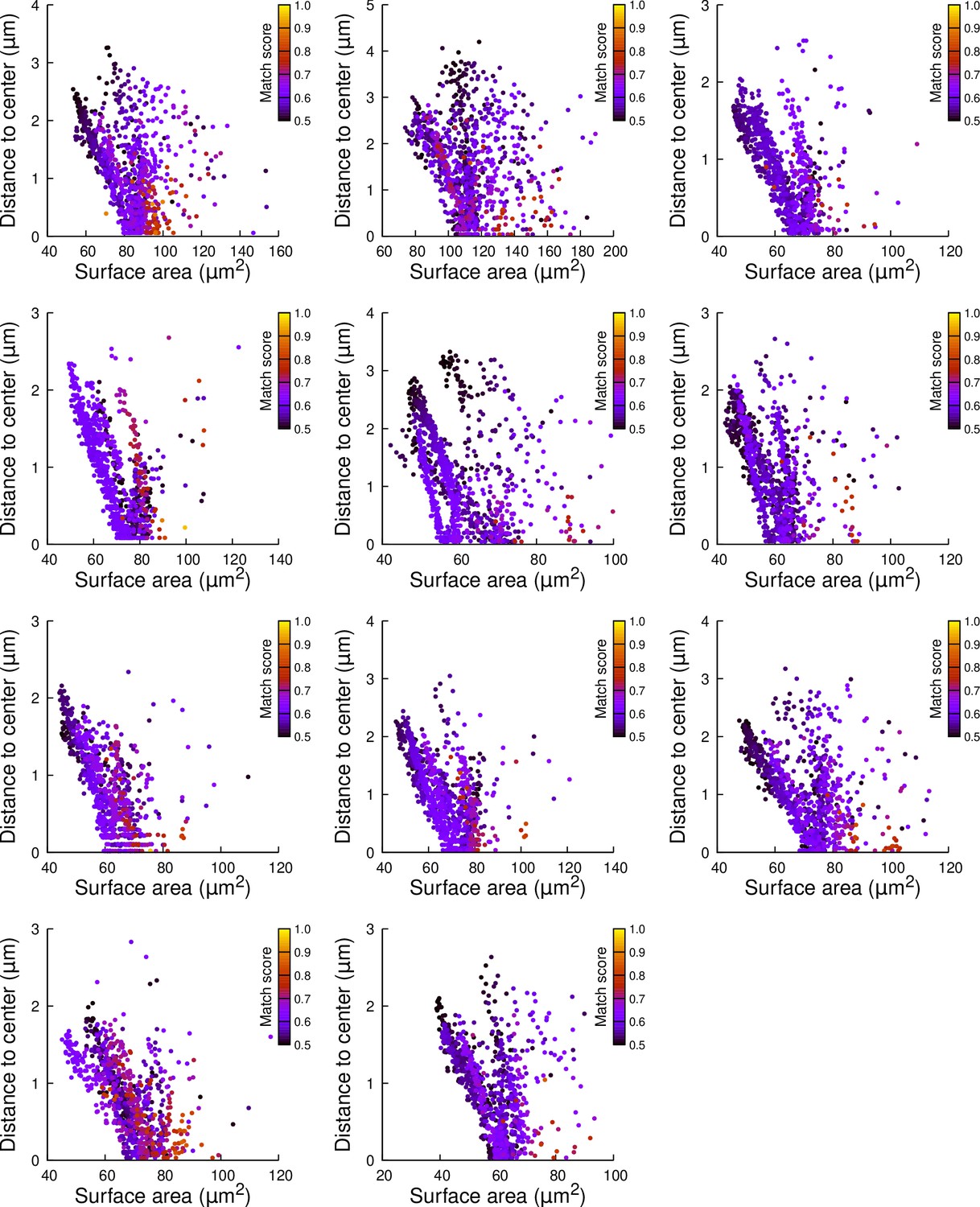
Figure 6—figure supplement 4
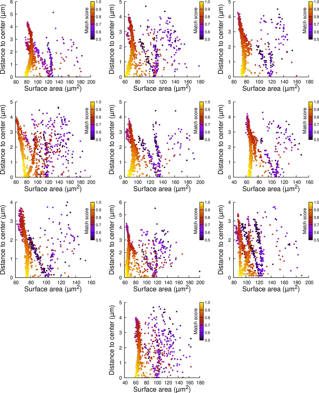
Results of cell division simulations at the 16C-32C transition in basal outer cells: distance to cell center as a function of plane surface area.
Each plot corresponds to a mother cell at generation 4 that was reconstructed by merging two observed sister cells at generation 5. Each dot corresponds to a simulated division in the mother cell. One thousand simulations at arbitrary volume-ratios were performed in each mother cell. Colors indicate the degree of matching between simulations and observed divisions.
Figure 6—figure supplement 5
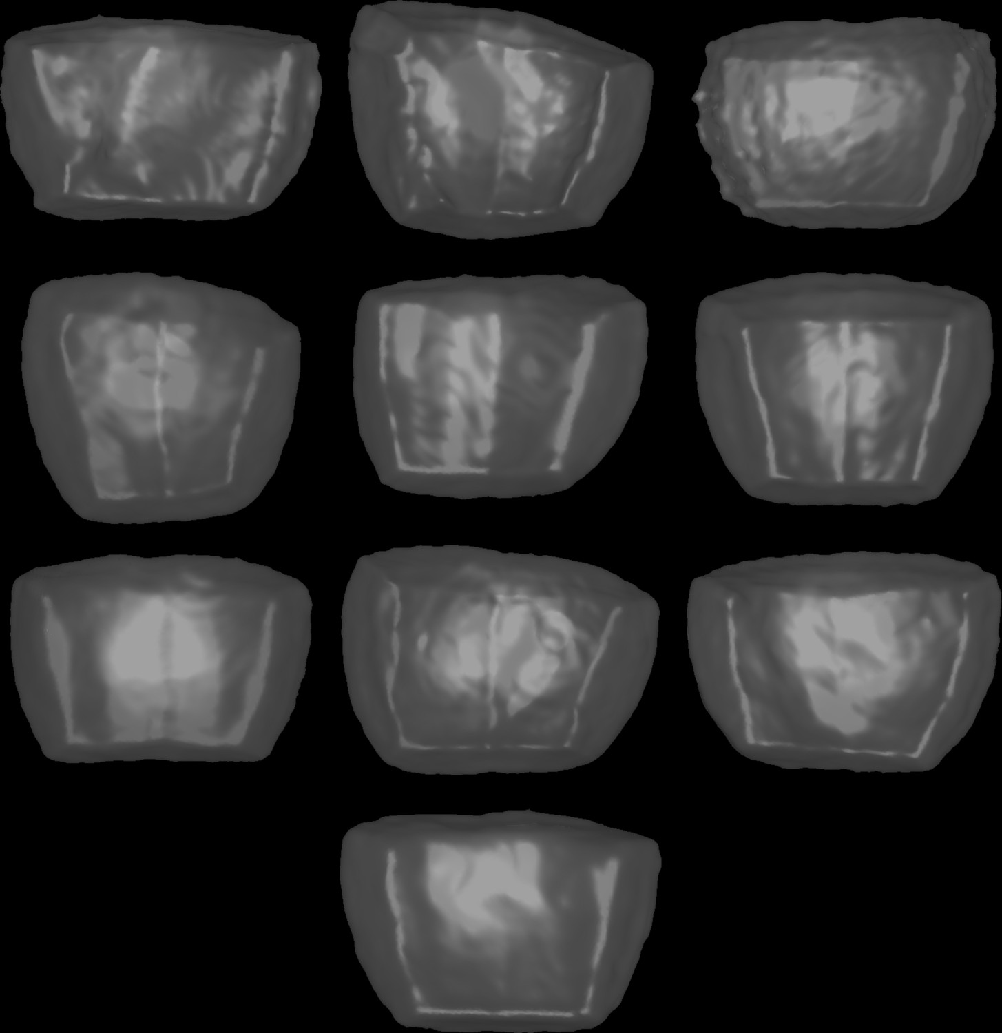
Mother cell shapes for simulations in basal outer cells.
These shapes were used for the simulations reported in Figure 6—figure supplement 4. Cells are shown from the outside of the embryo and displayed as transparent surfaces.
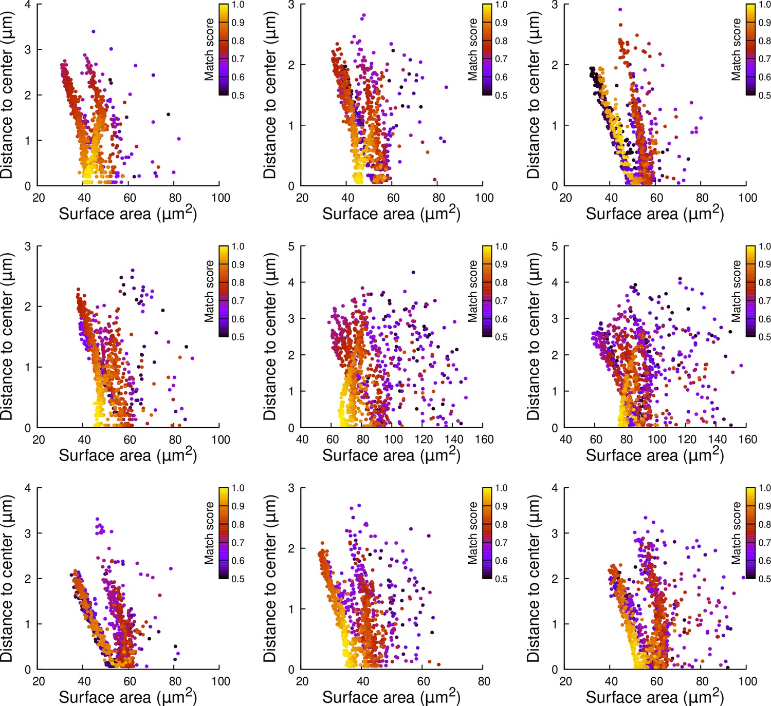
Figure 6—figure supplement 6
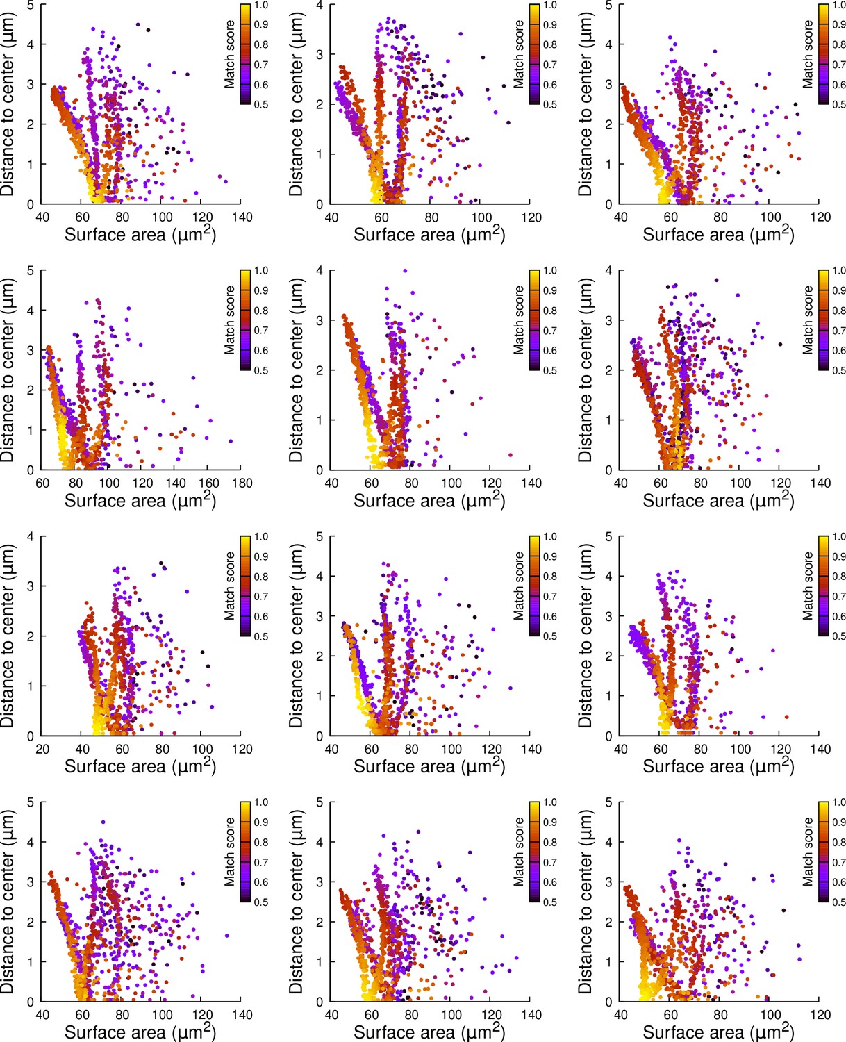
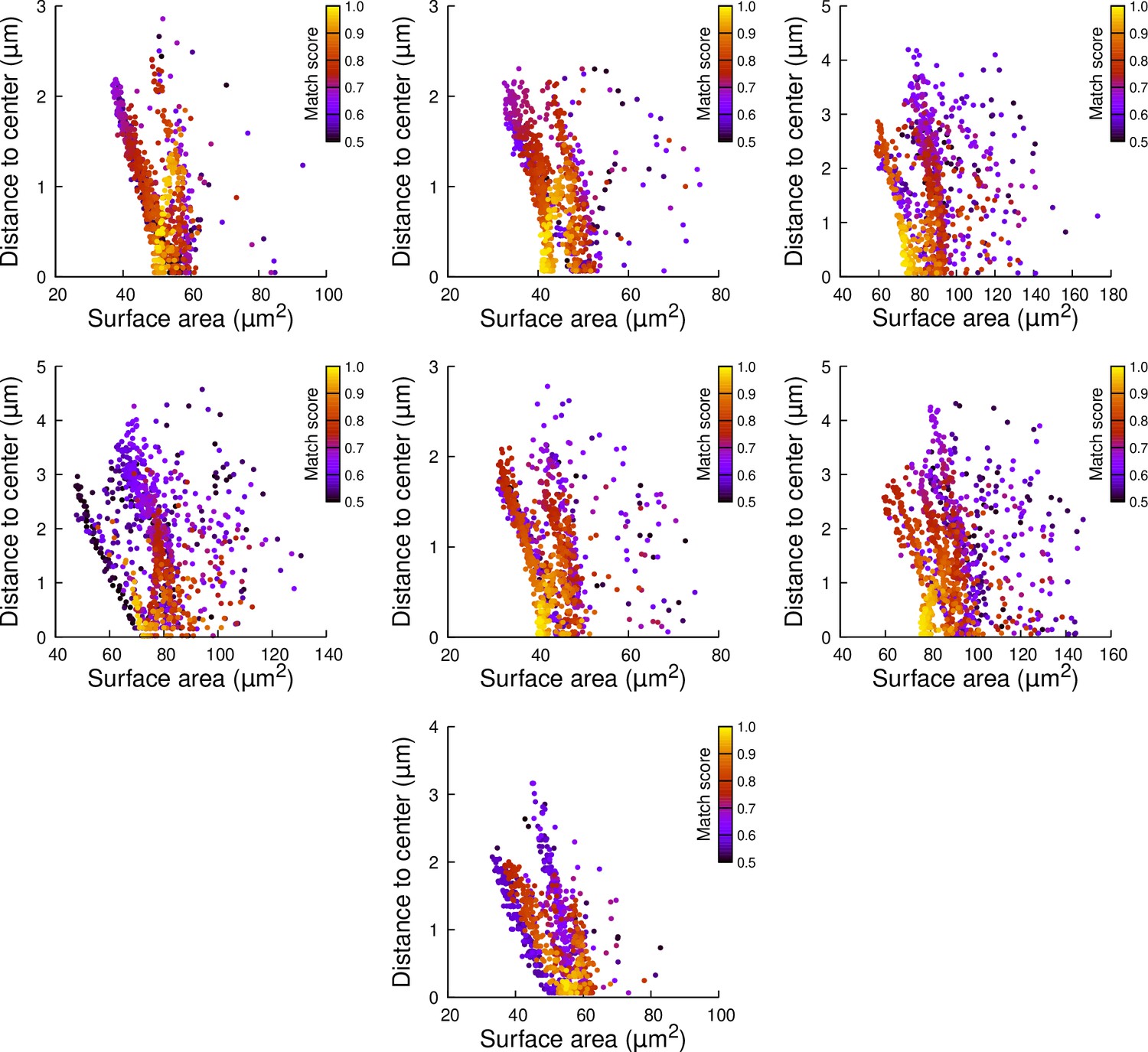
Results of cell division simulations at the 16C-32C transition in apical external cells dividing with a cuboid to the left: distance to cell center as a function of plane surface area.
Each plot corresponds to a mother cell at generation 4 that was reconstructed by merging two observed sister cells at generation 5. Each dot corresponds to a simulated division in the mother cell. One thousand simulations at arbitrary volume-ratios were performed in each mother cell. Colors indicate the degree of matching between simulations and observed divisions.
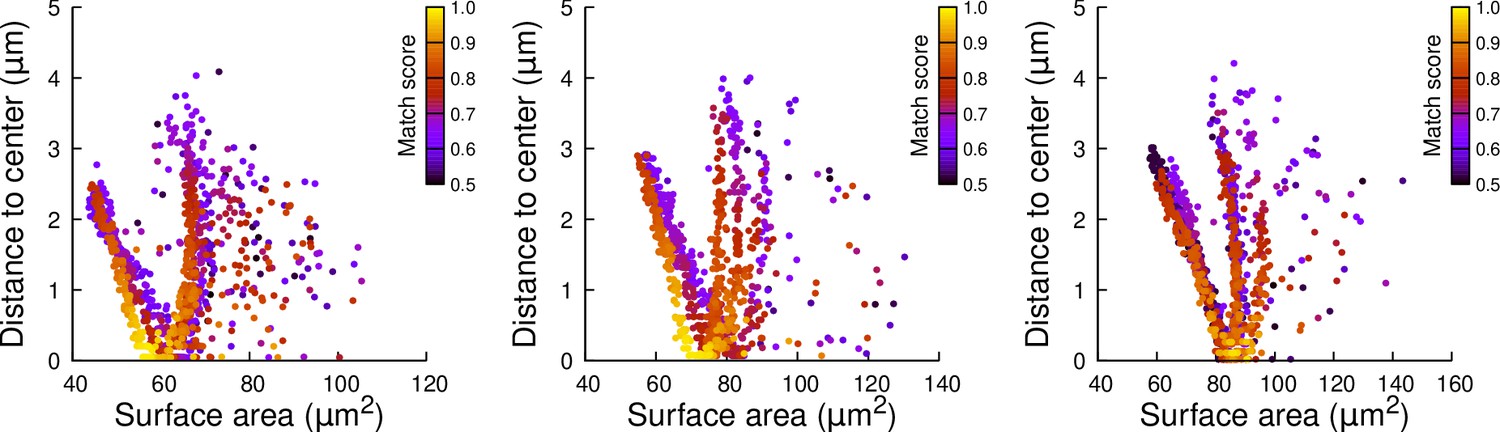
Figure 6—figure supplement 7
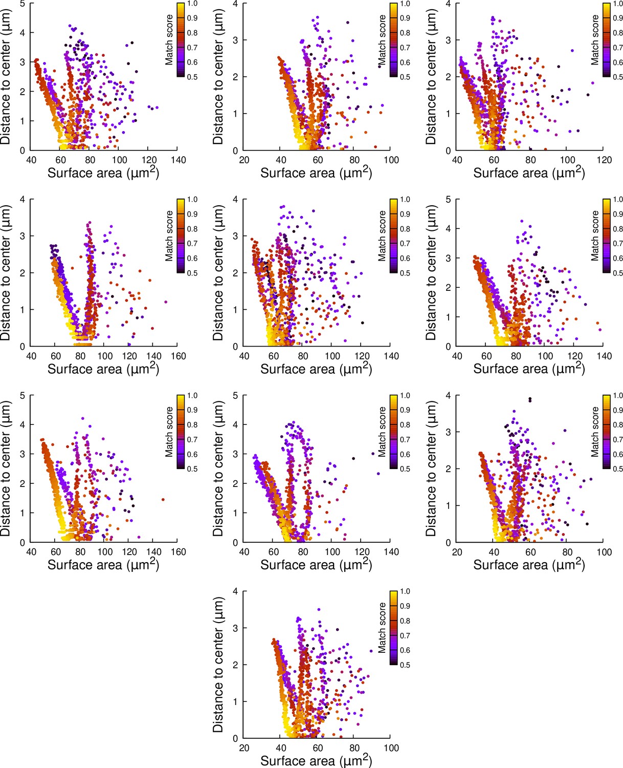
Results of cell division simulations at the 16C-32C transition in apical external cells dividing with a cuboid to the right: distance to cell center as a function of plane surface area.
Each plot corresponds to a mother cell at generation 4 that was reconstructed by merging two observed sister cells at generation 5. Each dot corresponds to a simulated division in the mother cell. One thousand simulations at arbitrary volume-ratios were performed in each mother cell. Colors indicate the degree of matching between simulations and observed divisions.
Figure 6—figure supplement 8
Results of cell division simulations at the 16C-32C transition in apical external cells dividing transversely: distance to cell center as a function of plane surface area.
Each plot corresponds to a mother cell at generation 4 that was reconstructed by merging two observed sister cells at generation 5. Each dot corresponds to a simulated division in the mother cell. One thousand simulations at arbitrary volume-ratios were performed in each mother cell. Colors indicate the degree of matching between simulations and observed divisions.
Figure 7 with 4 supplements
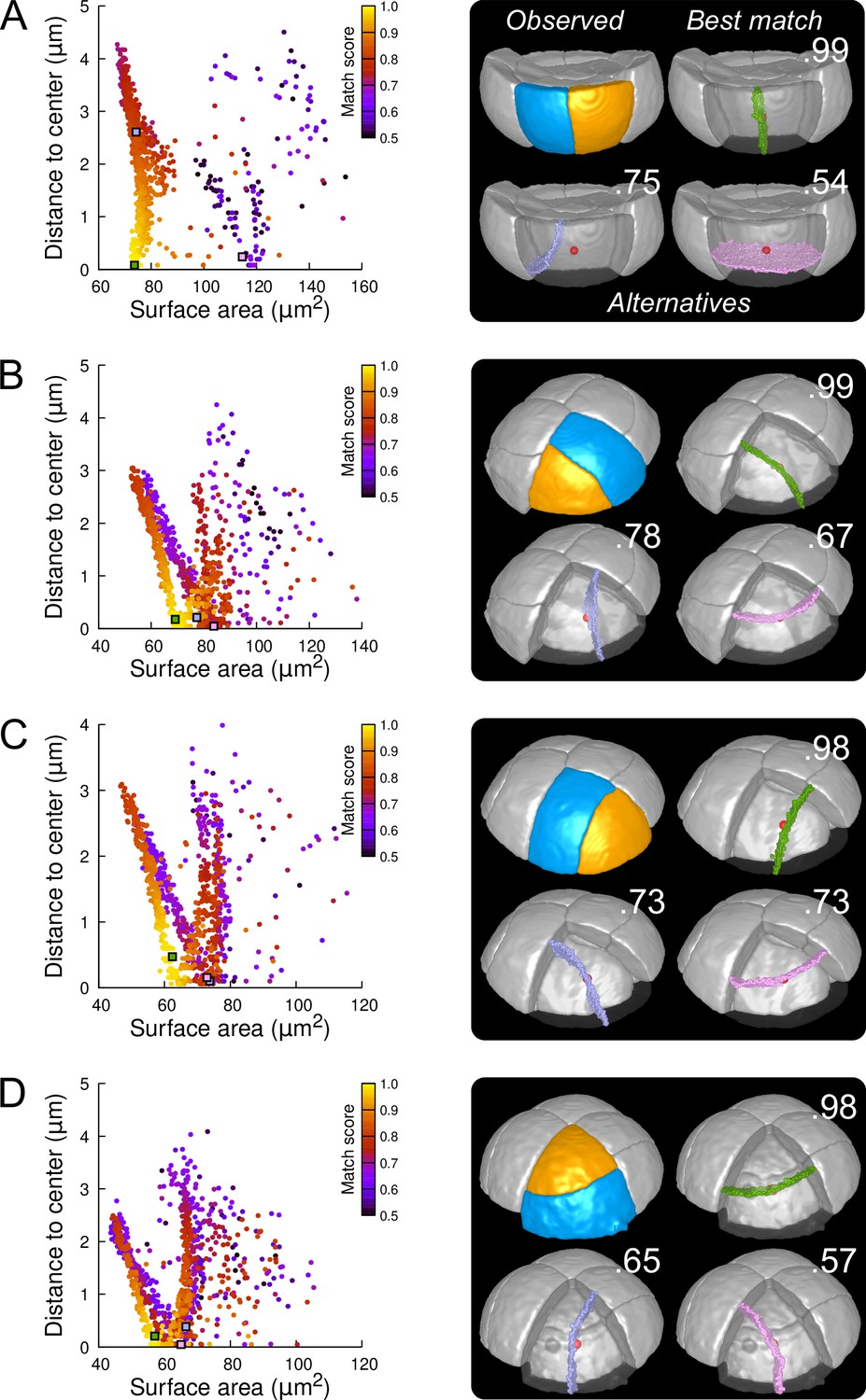
Modeling division patterns at G5 in internal cells based on geometrical features.
(A) Left: distribution plot of simulation results in a basal inner cell (N=1000). Simulated planes are positioned based on their surface area and distance to the mother cell center. The dot color indicates the match score between simulated and observed planes. Right: observed daughter cells (Blue and Orange); three simulated planes are shown in the reconstructed mother cell (Transparent). Green: simulation matching best with observed pattern. Lavender and Pink: simulations with alternative orientations. Numbers show the corresponding match scores. Red dot: mother cell center. In the dot plot (Left), the positions of the three simulated planes are shown as squares with the same colors. (BCD) Same as (A) for three apical inner cells.
Figure 7—figure supplement 1
Results of cell division simulations at the 16C-32C transition in basal inner cells: distance to cell center as a function of plane surface area.
Each plot corresponds to a mother cell at generation 4 that was reconstructed by merging two observed sister cells at generation 5. Each dot corresponds to a simulated division in the mother cell. One thousand simulations at arbitrary volume-ratios were performed in each mother cell. Colors indicate the degree of matching between simulations and observed divisions.
Figure 7—figure supplement 2
Results of cell division simulations at the 16C-32C transition in apical inner cells dividing with a triangular prism to the left: distance to cell center as a function of plane surface area.
Each plot corresponds to a mother cell at generation 4 that was reconstructed by merging two observed sister cells at generation 5. Each dot corresponds to a simulated division in the mother cell. One thousand simulations at arbitrary volume-ratios were performed in each mother cell. Colors indicate the degree of matching between simulations and observed divisions.
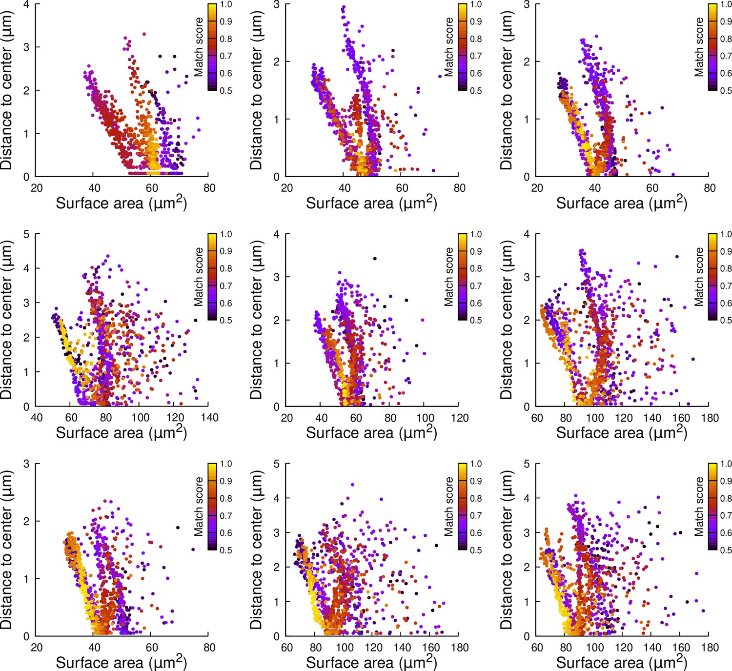
Figure 7—figure supplement 3
Results of cell division simulations at the 16C-32C transition in apical inner cells dividing with a triangular prism to the right: distance to cell center as a function of plane surface area.
Each plot corresponds to a mother cell at generation 4 that was reconstructed by merging two observed sister cells at generation 5. Each dot corresponds to a simulated division in the mother cell. One thousand simulations at arbitrary volume-ratios were performed in each mother cell. Colors indicate the degree of matching between simulations and observed divisions.
Figure 7—figure supplement 4
Results of cell division simulations at the 16C-32C transition in apical inner cells dividing longitudinally and radially: distance to cell center as a function of plane surface area.
Each plot corresponds to a mother cell at generation 4 that was reconstructed by merging two observed sister cells at generation 5. Each dot corresponds to a simulated division in the mother cell. One thousand simulations at arbitrary volume-ratios were performed in each mother cell. Colors indicate the degree of matching between simulations and observed divisions.
Figure 8
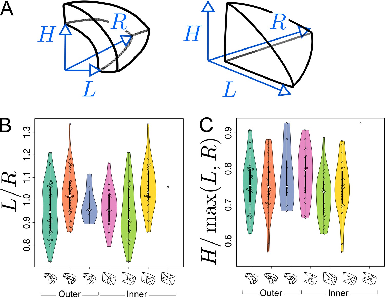
Asymmetries in mother cell geometry in the apical domain at stage 16C and their relations with division plane orientation.
(A) Measured lengths of outer (Left) and inner (Right) mother cells. : length along the longitudinal direction; and : lengths along the left and right radial directions. (B) Radial asymmetry. (C) Relative longitudinal length. Measurements were performed on mother cells reconstructed at G4/16C from observed embryos at G5 or G6.
-
Figure 8—source data 1
Left/right length ratio measurements.
- https://cdn.elifesciences.org/articles/79224/elife-79224-fig8-data1-v1.zip
-
Figure 8—source data 2
Longitudinal/radial length ratio measurements.
- https://cdn.elifesciences.org/articles/79224/elife-79224-fig8-data2-v1.zip
Figure 9
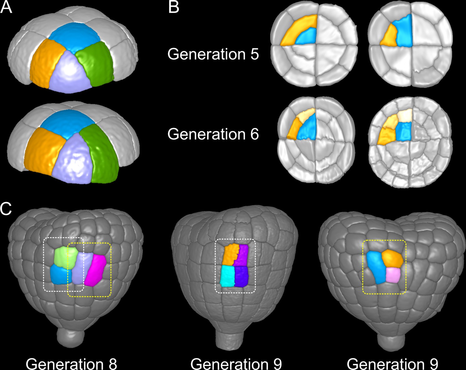
Attractor patterns buffer variability in division plane positioning.
(A) Similar cell patterns observed at G6 in the apical outer domain that have been reached through distinct cell division paths from G4. (B) Main (Left) and rare (Right) division patterns in the inner basal domain at G5 and corresponding patterns at G6. (C) Main (White box) and rare (Yellow) patterns observed at G8 and G9 in the outer basal domain.
Figure 10
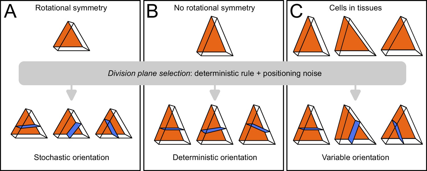
Schematic interpretation for the origin of variability in division patterns in Arabidopsis thaliana embryo.
A deterministic selection of division plane orientation, combined with noise in the precise positioning of the division plane, can generate variable orientation patterns. (A) In rotationnally symmetric cells, different orientations are statistically equivalent, inducing stochasticity at the individual cell level; symmetry is lost in daughter cells due to positioning noise. (B) In non-symmetric cells, a single orientation is selected. (C) Observed cells present asymmetries differently aligned with respect to the embryo axes, resulting in variable division patterns at the tissue scale.
Appendix 1—figure 1
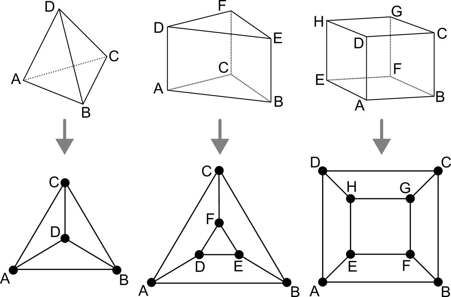
Polyhedral graphs (Bottom row) for the three main cell shapes (Top row) found in Arabidopsis thaliana early embryogenesis.
Note that in these representations (Schlegel diagrams), the outside counts as one face of the corresponding polyhedron.
Appendix 1—figure 2
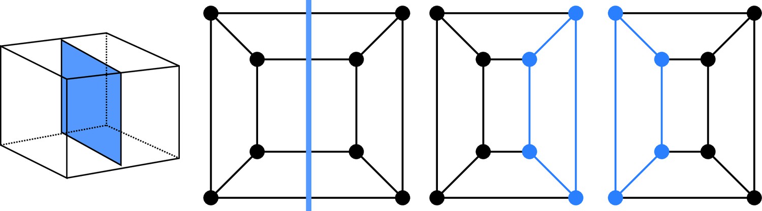
Cell division as cuts on polyhedral graphs: illustration with the division of a cuboid.
The division on the left corresponds to the edge cut shown in the middle. Completing the two subgraphs of this cut with nodes and edges (Blue) yields the two subgraphs of the daughter cells. The obtained subgraphs correspond to two cuboids, as expected for the considered division.
Tables
Appendix 1—table 1
Divisions of the tetrahedral cell shape (4.6.4).
| 1/3 | 2/2 | |
|---|---|---|
| 4 | 3 | |
| -shape | 4.6.4 | 6.9.5 |
| -shape | 6.9.5 | 6.9.5 |
Appendix 1—table 2
Divisions of the triangular prismatic cell shape (6.9.5).
refers to the case where the -subgraph is acyclic, to the case where it is cyclic.
| 1/5 | 2/4 | 3/3α | 3/3β | |
|---|---|---|---|---|
| 6 | 9 | 12 | 1 | |
| -shape | 4.6.4 | 6.9.5 | 8.12.6 | 6.9.5 |
| -shape | 8.12.6 | 8.12.6 | 8.12.6 | 6.9.5 |
Appendix 1—table 3
Divisions of the cuboidal cell shape (8.12.6).
refers to the case where the -subgraph is acyclic, to the case where it is cyclic.
| 1/7 | 2/6 | 3/5 | 4/4α | 4/4β | |
|---|---|---|---|---|---|
| 8 | 12 | 18 | 4 | 3 | |
| -shape | 4.6.4 | 6.9.5 | 8.12.6 | 10.15.7 | 8.12.6 |
| -shape | 10.15.7 | 10.15.7 | 10.15.7 | 10.15.7 | 8.12.6 |
Additional files
Download links
A two-part list of links to download the article, or parts of the article, in various formats.
Downloads (link to download the article as PDF)
Open citations (links to open the citations from this article in various online reference manager services)
Cite this article (links to download the citations from this article in formats compatible with various reference manager tools)
Large-scale analysis and computer modeling reveal hidden regularities behind variability of cell division patterns in Arabidopsis thaliana embryogenesis
eLife 11:e79224.
https://doi.org/10.7554/eLife.79224


