Figures and data in Cellular compartmentalisation and receptor promiscuity as a strategy for accurate and robust inference of position during morphogenesis

Figures
Tables
Additional files

30 figures, 3 tables and 1 additional file

Figures

Figure 1

Download asset Open asset

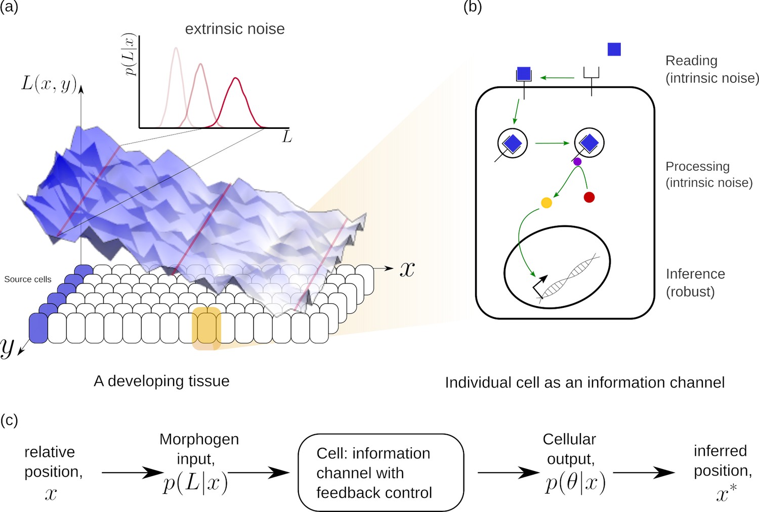
Schematic of information processing in the developing tissue.

(a) A morphogen is produced by a specific set of cells (blue), and secreted into the lumen surrounding the tissue. Due to stochasticity of the production and transport processes, the morphogen concentration received by the rest of the cells is contaminated by *extrinsic noise*, which defines a distribution of morphogen concentration along the $y$ -direction at any position $x$ . (b) The route from morphogens to a developmental outcome requires each cell to read, process and infer its position. This task is further complicated by the stochasticity of the reading and processing steps themselves, that lead to *intrinsic noise*. (c) The problem of robust inference of position can be considered in a channel framework. The positional information is noisily encoded in the local morphogen (ligand) concentrations, $p (L | x)$ . The cells receive this as input and process it into a less noisy output to ensure robustness in inferred positions.

Figure 2

Download asset Open asset

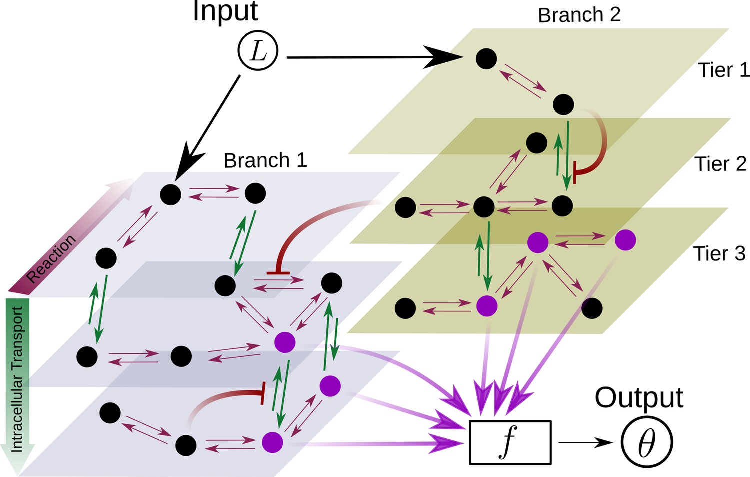
Schematic for the branch-tier channel architecture.

*Branches* correspond to different receptor types and *tiers* denote the layers of compartmentalisation used in cellular processing. Cellular processing associated with each receptor type (here, branches 1 and 2) is depicted by a generic Markov network. The gray and brown planes depict the tiers in the two branches respectively (here, tiers 1, 2, and 3 in each branch). The bi-directional in-plane purple arrows correspond to faster transitions between receptor states, e.g. bound/unbound, and the green bi-directional arrows depict slower transitions involving intracellular transport driven by flux-imbalanced processes. There may exist several feedback control loops (red ━┥ arrows) in the network. Ligand concentration $L$ drives one or several reaction rates in such Markov networks as in Harvey et al., 2020. The output $θ$ is a collection $f$ of several signalling states (purple nodes) from one or many branches. The statistics of the output $θ$ then enables inference of position.

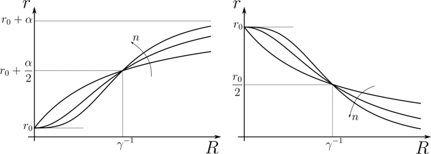
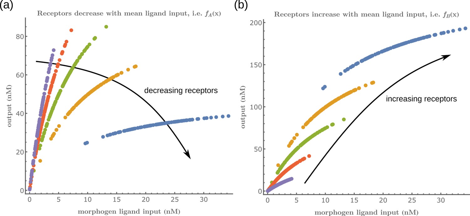
Figure 3

Download asset Open asset

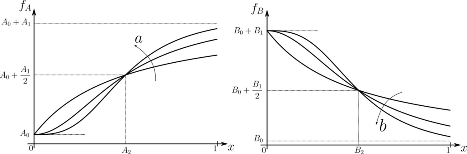
Family of receptor profiles $f_{A}$ (monotonically increasing in $x$ ) and $f_{B}$ (monotonically decreasing in $x$ ) with an interpretation of function parameters (Equations 8; 9).

The total surface concentrations of both signalling and non-signalling receptors are taken from these families of receptor profiles.

Figure 4

Download asset Open asset

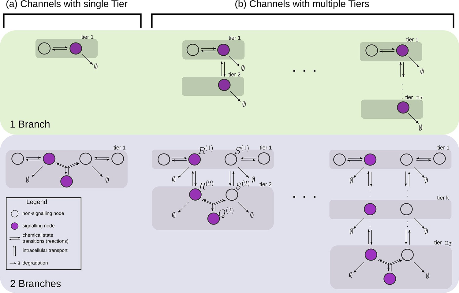
Examples of channel architectures with single and multiple tiers, and upto two branches.

Signalling receptors in the bound state (colour purple) from each of the tiers contribute to the cellular output. The interpretation of the arrows is shown in the legend.

Figure 5

Download asset Open asset

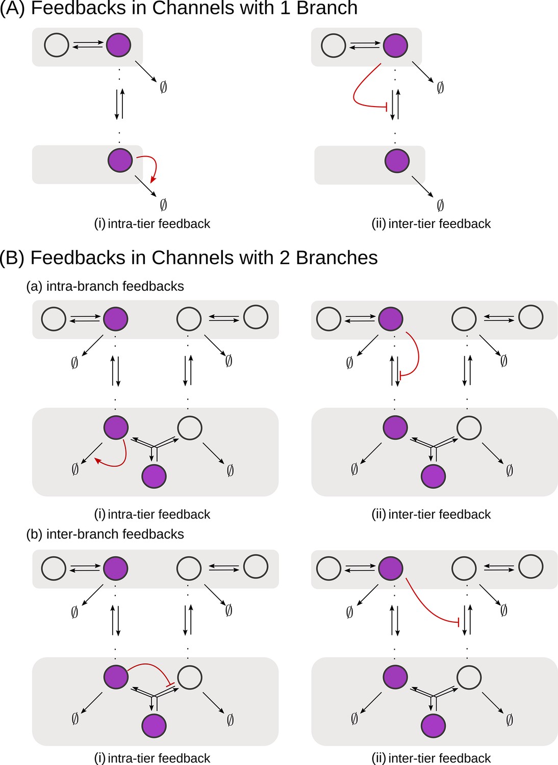
Schematic of feedback types.

(A) In a one-branch channel, feedbacks are considered on internalisation rates or degradation rates. (B) A second branch in the channel opens up the possibilities of (a) intra-branch and (b) inter-branch, (i) intra-tier and (ii) inter-tier feedbacks.

Figure 6

Download asset Open asset

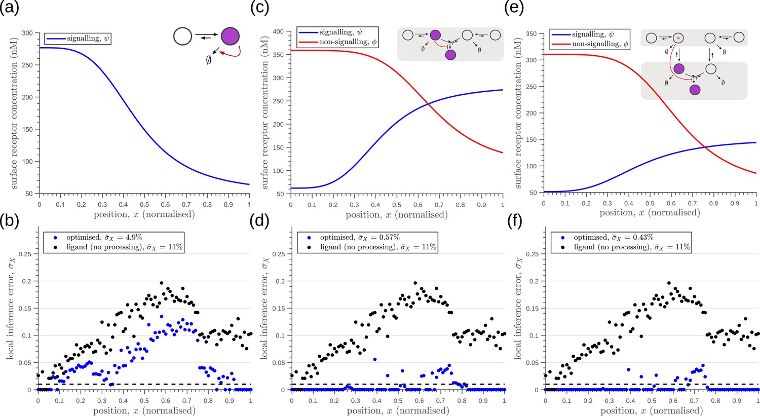
Characteristics of an optimised (a) one-tier one-branch channel with only the signalling receptor and feedback.

The optimised channel shows a moderately strong positive feedback on the degradation rate. (b) The optimal output is obtained when (b, inset) the total (bound plus unbound) signalling receptor concentration profile decreases away from the source. (c) Local inference errors in this optimised channel show a reduction compared to the expected inference errors from ligand with no cellular processing (i.e. reading directly from the free ligand). The minimum average inference error in this channel is ${\bar{σ}}_{X} \sim 8 %$ , which corresponds to 8 cells’ width. The dashed line denotes a local inference error of one cell’s width $\sim 1 / n_{x}$ . (d) The input-output relations in this channel are monotonically increasing sigmoid functions saturating at only large values of input. The solid lines correspond to the input-output relations at selected positions $x = 0.25, 0.5, 0.75$ , shaded with the same colour as the position-markers in (b inset, coloured rectangles). The signalling $ψ (x)$ receptor concentration is mentioned in the legend. For a fixed distribution of ligand input (Equation 1), the range of input values recorded by the receptors at the selected positions gives rise to a range of outputs (circles). It is clear that neighbouring positions have significant overlaps in their outputs. The optimised parameter values for the plots in (**b–d**) can be found in Table 2 under the column corresponding to $n_{T} = 1, n_{B} = 1, r_{+} = r_{d}^{(1)}$ .

Figure 7

Download asset Open asset

Results of optimisation of (a) one-tier two-branch channel.

(b) The output profile (with standard error in shaded region) corresponding to the (inset) optimised signalling (blue) and non-signalling (red) receptor profiles. The optimal signalling receptor now increases away from the source as opposed to the situation in the optimal one-tier one-branch channel (Figure 6). On the other hand, the optimal non-signalling receptor decreases away from the source. (c) The local inference error $σ_{X} (x)$ is reduced throughout the tissue, when compared to the expected inference errors from ligand with no processing. (d) The input-output relations at selected positions $x = 0.25, 0.5, 0.75$ (in the direction of the black arrow) are shown as solid lines, shaded with the same colour as the position-markers in (b inset, coloured rectangles). The signalling $ψ (x)$ and non-signalling $ϕ$ receptor concentrations are mentioned in the legend. For a fixed distribution of ligand input (Equation 1), the range of input values recorded by the receptors at the selected positions gives rise to a range of outputs (circles). Tuning of input-output relations through receptor concentrations reduces output variance and minimises overlaps in the outputs of neighbouring cell cohorts. The optimised parameter values for the plots in (**b–d**) can be found in Table 2 under the column corresponding to $n_{T} = 1, n_{B} = 2, r_{-} = κ_{C}$ .

Figure 8

Download asset Open asset

Performance of the optimised two-branch channels with increasing numbers of tiers.

(a) Minimum average inference error ${\bar{σ}}_{X}$ in two-branch architectures with increasing number of tiers $n_{T}$ . The dashed line corresponds to a local inference error of one cell’s width $\sim 1 / n_{x}$ . (**b,c**) Results of optimisation of two-tier two-branch channels with inter-branch feedback. These two architectures perform equally well: local inference errors in both the channels (blue dots) are low throughout the tissue (with average inference errors $\sim 1.6 %$ and $\sim 1.7 %$ ) as compared to a case with no processing of ligand prior to inference (black dots). Note that the local inference errors in the optimised channels increase towards the end of the tissue due to lower ligand concentrations. The dashed line corresponds to a local inference error of one cell’s width $\sim 1 / n_{x}$ . The optimised parameter values for the plots in (**b–c**) can be found in Table 2 under the column corresponding to $n_{T} = 2, n_{B} = 2, r_{-} = κ_{I}$ and $n_{T} = 2, n_{B} = 2, r_{-} = κ_{C}$ , respectively.

Figure 9

Download asset Open asset

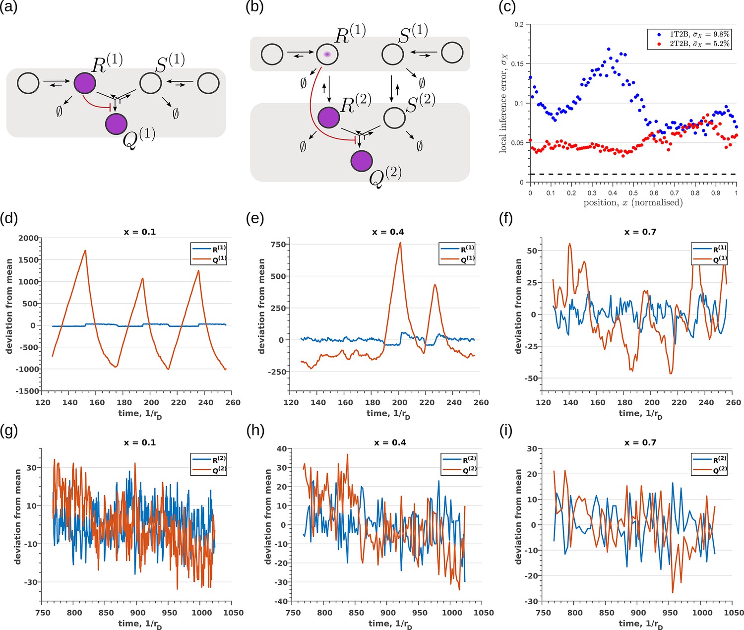
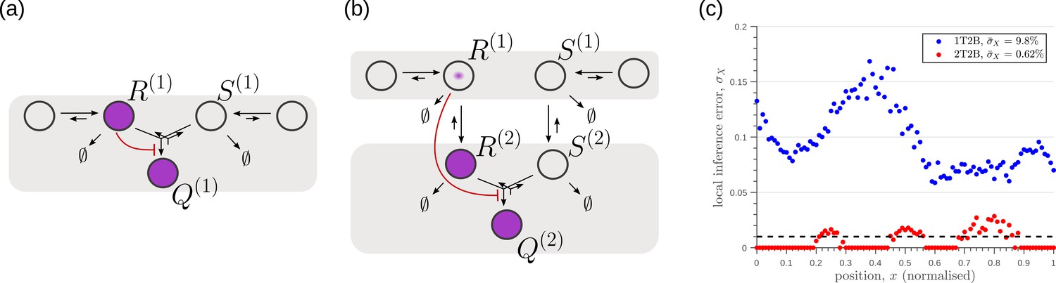
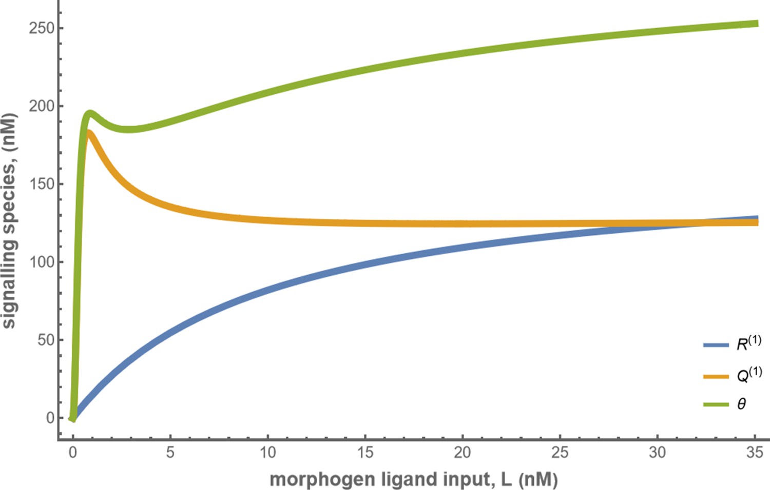
Robustness to intrinsic noise in (a) one-tier two-branch (1T2B) channel and (b) two-tier two-branch (2T2B) channel architectures, previously optimised for extrinsic noise alone.

(c) A comparison of local inference errors due to intrinsic noise shows consistently better performance in the case of a two-tier two-branch channel (red dots). (**d-f**) Sample steady-state trajectories of the signalling species $R^{(1)}$ (blue) and $Q^{(1)}$ (red) of a one-tier two-branch channel (purple nodes in (a)) at positions $x = 0.1, 0.4, 0.7$ , respectively. (**g–i**) Sample steady-state trajectories of the signalling species $R^{(2)}$ (blue) and $Q^{(2)}$ (red) of a two-tier two-branch channel (purple nodes in (b)) at positions $x = 0.1, 0.4, 0.7$ , respectively. The optimised parameter values for the plots in (**c,d–f,g–i**) can be found in Table 2 under the column corresponding to $n_{T} = 1, n_{B} = 2, r_{-} = κ_{C}$ and $n_{T} = 2, n_{B} = 2, r_{-} = κ_{C}$ , respectively.

Figure 10

Download asset Open asset

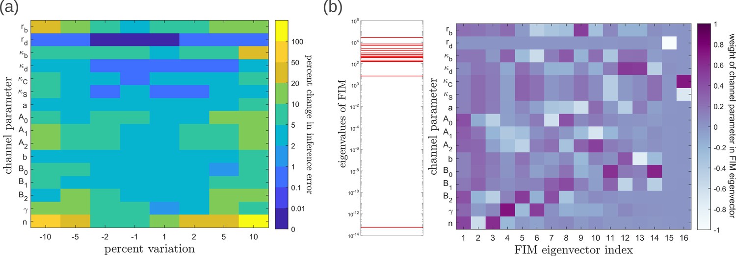
Geometry of the fidelity landscape around the optimum.

(a) Percent changes in the inference error upon perturbations in the channel parameters (as described in Table 1) around the optimum for one-tier two-branch channel (optimised ${\bar{σ}}_{X} = 1.9 %$ ). For most perturbations, the inference error deviates by up to 20% of the optimum i.e. the inference error ${\bar{σ}}_{X}$ remains below 2.2%. (b) *Left:* eigen spectrum of the Fisher information metric (FIM, see Equation 21) around the global minimum of ${\bar{σ}}_{X}$ , *Right:* weight of the different channel parameters in the eigenvectors of FIM, obtained from projecting each eigenvector along the channel parameter axes. The index 1 corresponds to the eigenvector with the largest eigenvalue and the index 16 corresponds to the eigenvector with the smallest eigenvalue.

Figure 11

Download asset Open asset

Geometry of the low inference error landscape defined by channels within a band ${\bar{σ}}_{X} \leq 2 %$ about the global minimum.

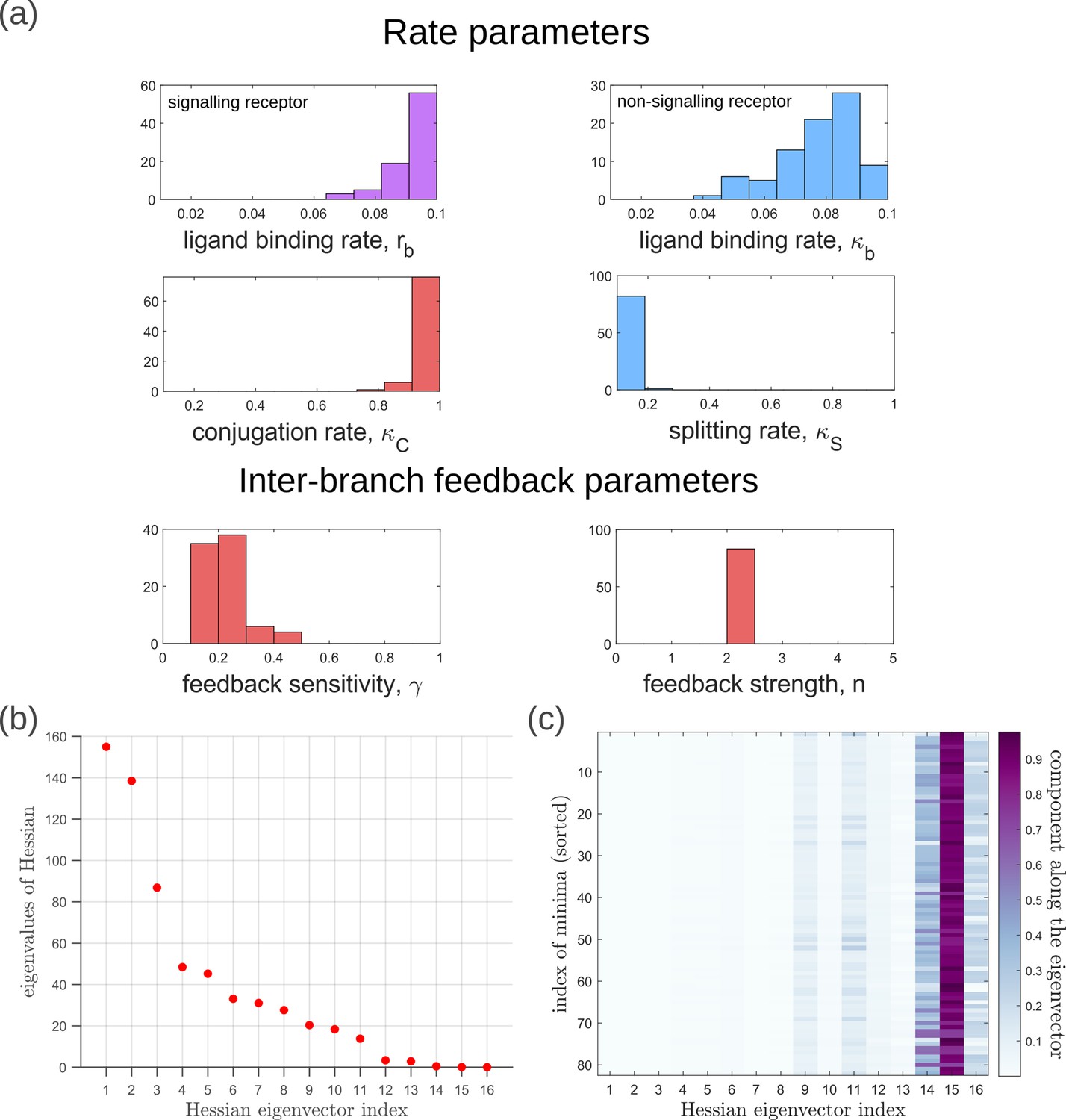
(a) Frequency distributions of optimised channel parameters in the low inference error landscape. Here we show the ligand binding rates of the signalling and non-signalling receptors, conjugation and splitting rates, and feedback sensitivity and feedback strength parameters. The distributions of the other optimised channel parameters are shown in Appendix 14. (b) Eigenvalues of the Hessian $h_{μ ν}$ (see Equation 22) of ${\bar{σ}}_{X}$ around the global minimum. (c) Components of the normalised ‘position vectors’ of the minima ${\vec{v}}^{opt} \in V$ along the eigenvectors of the Hessian $h_{μ ν}$ , obtained from projecting each position vector along the eigenvector of the Hessian. Here, position vectors in the parameter space $V$ are defined by the usual Euclidean metric.

Figure 12

Download asset Open asset

Robustness to extrinsic noise with a different choice of objective function (Equation 23) for one-tier one-branch channel (**a–b**), one-tier two-branch channel (**c–d**) and two-tier two-branch channel (**e–f**).

(a) Profile of the signalling receptor for (a, inset) the optimised one-tier one-branch channel. (b) Corresponding inference errors due to extrinsic noise in the optimised one-tier one-branch channel. (c) Profiles of the signalling (blue) and non-signalling (red) receptor for (c, inset) the optimised one-tier two-branch channel. (d) Corresponding inference errors due to extrinsic noise in the optimised one-tier two-branch channel. Errors are predominantly located around the segment boundaries at $x = 0.25, 0.5, 0.75$ and still increase in the direction of reducing morphogen concentrations. (e) Profiles of the signalling (blue) and non-signalling (red) receptor for (e, inset) the optimised two-tier two-branch channel. (f) Corresponding inference errors due to extrinsic noise in the optimised two-tier two-branch channel. Note that the errors here are predominantly around the segment boundaries ( $x = 0.25, 0.5, 0.75$ ) and diminished compared to the one-tier two-branch channel in (d).

Figure 13

Download asset Open asset

Robustness to intrinsic noise, with a different choice of objective function (Equation 23), in (a) one-tier two-branch (1T2B) channel and (b) two-tier two-branch (2T2B) channel architectures, previously optimised for extrinsic noise alone.

(c) A comparison of local inference errors of the two optimised channels in (**a,b**) in presence of intrinsic noise. Even for this choice of objective function, the two-tier channel shows consistently better performance.

Figure 14 with 1 supplement

Download asset Open asset

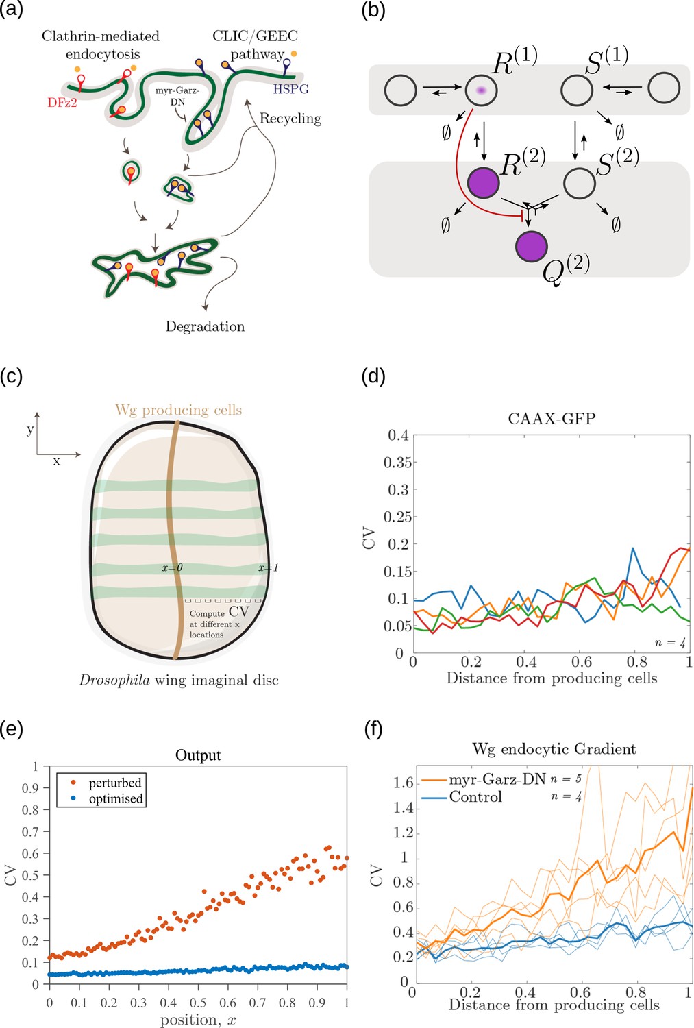
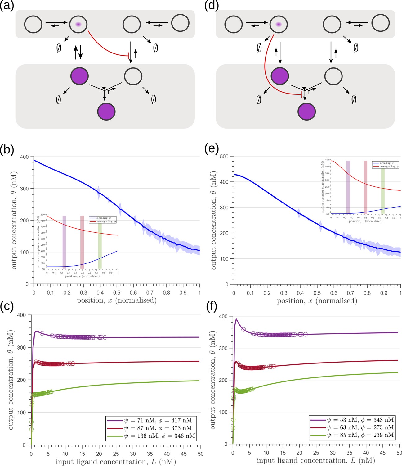
Comparison of theoretical results with experimental observations on Wg signalling system in *Drosophila* wing imaginal disc.

(a) Schematic of the cellular processes involved in Wg signalling, showing the two endocytic routes for the receptors (see text for further description). (b) Two-tier two-branch channel architecture corresponding to the Wg signalling system. (c) Schematic describing the XY view of wing disc. The vertical brown stripe marks the Wg producing cells. Horizontal green stripes mark the regions in wing disc used for analysis. See *Experimental Methods* (Appendix 15) for more information. (d) Coefficient of variation (CV) of CAAX-GFP intensity profiles, expressed in wing discs, as a function of (normalized) distance from producing cells (n=4). (e) Coefficient of variation in the output of the optimised two-tier two-branch channel (blue), and upon perturbation (orange) via removal of the non-signalling branch, implemented by setting all rates in the non-signalling branch $κ$ to zero. The optimised parameter values for the plot can be found in Table 2 under the column corresponding to $n_{T} = 2, n_{B} = 2, r_{-} = κ_{C}$ . (f) CV of intensity profiles of endocytosed Wg in control wing discs (C5GAL4Xw1118; blue; n=4) and discs where CLIC/GEEC endocytic pathway is removed using UAS-myr-garz-DN (C5GAL4XUAS-myr-garz-DN; orange; n=5).

Figure 14—source data 1 CV of intensity measurements of CAAX GFP and endocytosed Wg, in control and myr-Garz-DN, as a function of distance from producing cells in individual samples of wing imaginal discs.: https://cdn.elifesciences.org/articles/79257/elife-79257-fig14-data1-v1.xlsx
Download elife-79257-fig14-data1-v1.xlsx

Figure 14—figure supplement 1

Download asset Open asset

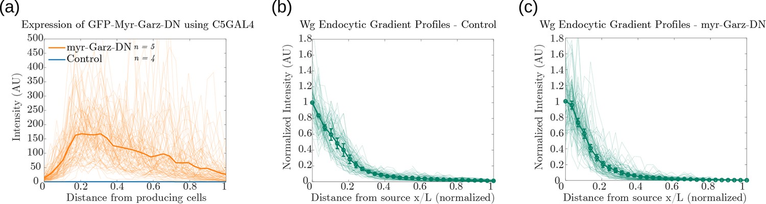
Supporting measurements of fluorescence intensity profiles for Figure 14d and Figure 14f.

Fluorescence intensity profiles of: (a) GFP-Myr-Garz-DN and control. Endocytosed Wg profiles in (b) control wing discs (n=4) and (c) discs where CLIC/GEEC endocytic pathway is removed using UAS-myr-Garz-DN (n=5). Figure 14—figure supplement 1—source data 1.Fluorescence intensity measurements for a-c. Mean and standard error of mean (SEM) for b,c. Figure 14—source data 1.CV of intensity measurements of CAAX GFP and endocytosed Wg, in control and myr-Garz-DN, as a function of distance from producing cells in individual samples of wing imaginal discs.

Figure 14—figure supplement 1—source data 1 Fluorescence intensity measurements for a-c. Mean andstandard error of mean (SEM) for b,c.: https://cdn.elifesciences.org/articles/79257/elife-79257-fig14-figsupp1-data1-v1.xlsx
Download elife-79257-fig14-figsupp1-data1-v1.xlsx

Appendix 2—figure 1

Download asset Open asset

Hill functions representing positive (left) and negative (right) feedback control on chemical rates $r$ actuated by chemical species $R$ .

The effect of feedback amplification $α$ , sensitivity $γ$ and strength $n$ are indicated. r₀ denotes the reference value of the chemical rate $r$ in absence of feedback.

Appendix 4—figure 1

Download asset Open asset

Schematic of an *ideal* output profile.

The monotonically decreasing curve is the mean output profile. Due to various sources of noise, the output at any point will have a distribution around the local mean. If neighbouring cohorts of cells are to accurately distinguish their inferred positions from their outputs (in the Bayesian sense), the output distributions must have a small overlap (shaded region under the distribution curves).

Appendix 4—figure 2

Download asset Open asset

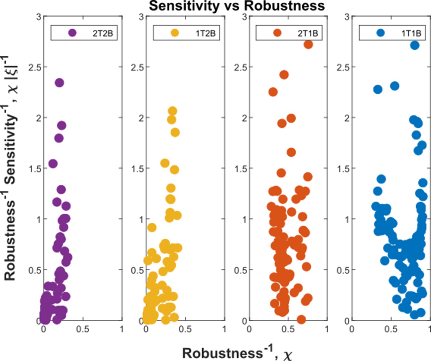
Robustness-Sensitivity plots for $n_{x} - 1 = 100$ cohorts in the optimised channel architectures.

The robustness-sensitivity objective is to reach the origin along both the axes. Optimised single-branch architectures (labelled 1T1B and 2T1B) show the two measures as conflicting objectives, such that improvement in robustness is achieved at the expense of sensitivity beyond a certain point. This conflict is absent in the optimised two-branch architectures (labelled 1T2B and 2T2B). An additional tier in two-branch architectures can further improve the two local measures. Note: the choice of coordinate axes reflects the requirement of simultaneous minimisation of $χ$ (Equation 32) and $ξ^{- 1}$ (Equation 33) and the allowed tolerance in $ξ^{- 1}$ when $χ$ is below a certain level.

Appendix 4—figure 3

Download asset Open asset

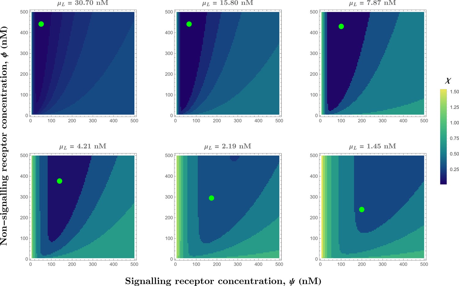
Contour plots of $χ$ (see Eq.Equation 32) in the optimised one-tier two-branch channel with inter-branch feedback control (Figure 7a of the main text) showing the preferred receptor combinations (deep blue) for different values of mean input $μ_{L}$ .

Green dots denote the receptor concentrations in the optimised channel (Figure 7b,inset of the main text) at positions corresponding to the values of mean input $μ_{L}$ indicated above the contour plots. The optimised parameter values for the plots can be found in Table 2 under the column corresponding to $n_{T} = 1, n_{B} = 2, r_{-} = κ_{C}$ .

Appendix 4—figure 4

Download asset Open asset

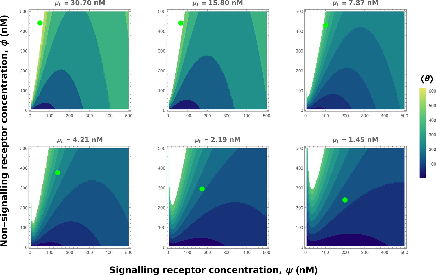
Contour plots of mean output $⟨ θ ⟩$ in the optimised one-tier two-branch channel with inter-branch feedback control (Figure 7a of the main text).

The contours move downward along the axis of the non-signalling receptor $ϕ$ . Therefore, as the preferred values of signalling receptor $ψ$ decrease with mean ligand input $μ_{L}$ (Appendix 4—figure 3), non-signalling receptor concentration $ϕ$ needs to increase with $μ_{L}$ to ensure that the mean output $⟨ θ ⟩$ is a monotonically increasing function of. $μ_{L}$ Green dots denote the receptor concentrations in the optimised channel (Figure 7b,inset of the main text) at positions corresponding to the values of mean input $μ_{L}$ indicated above the contour plots. The optimised parameter values for the plots can be found in Table 2 under the column corresponding to. $n_{T} = 1, n_{B} = 2, r_{-} = κ_{C}$

Appendix 5—figure 1

Download asset Open asset

Input-Output function of a *minimal* channel shows the importance of choosing the correct receptor profiles.

Appendix 6—figure 1

Download asset Open asset

Concentrations of the signalling species $R^{(1)}, Q^{(1)}$ and total cellular output $θ$ in the optimised one-tier two-branch channel with $ψ = 164 nM, ϕ = 318 nM$ .

The optimised chemical rates and feedback parameters for the above plot can be found in Table 2 under the column corresponding to $n_{T} = 1, n_{B} = 2, r_{-} = κ_{C}$ .

Appendix 8—figure 1

Download asset Open asset

Results of optimisation of (**a,d**) two-tier two-branch channels.

(**b,e**) The output profiles (with standard error in shaded region) and (insets) the corresponding optimised signalling (blue) and non-signalling (red) receptor profiles. (**c,f**) The input-output relations at selected positions $x = 0.25, 0.5, 0.75$ are shown as solid lines, shaded with the same colour as the position-markers (coloured rectangles in b,e insets). The signalling $ψ (x)$ and non-signalling $ϕ$ receptor concentrations are mentioned in the legend. For a fixed distribution of ligand input (Equation 1), the range of input values recorded by the receptors at the selected positions gives rise to a range of outputs (circles). Tuning of input-output relations through receptor concentrations reduces output variance and minimises overlaps in the outputs of neighbouring cell cohorts. The optimised parameter values for the plots in (**b–c,e–f**) can be found in Table 2 under the column corresponding to $n_{T} = 2, n_{B} = 2, r_{-} = κ_{I}$ and $n_{T} = 2, n_{B} = 2, r_{-} = κ_{C}$ , respectively.

Appendix 9—figure 1

Download asset Open asset

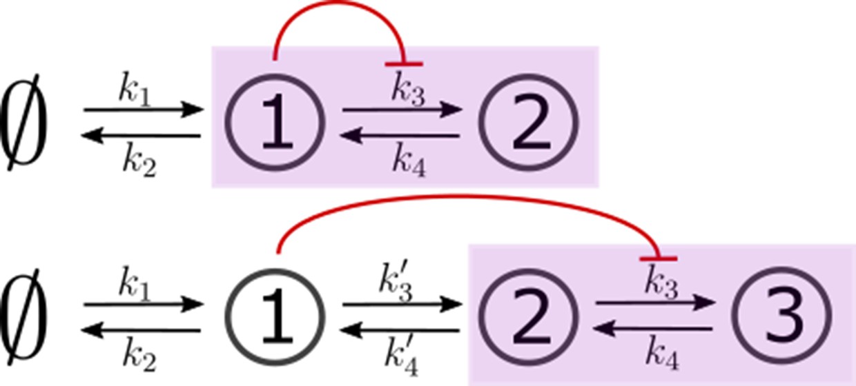
Two- and three-species CRNs with production k₁ and degradation k₂ rates of species 1 (s₁) and inter-conversion $k_{3}, k_{4}$ rates between the “signalling" (output generating) species (in purple box).

These rates mimic the binding r_b, unbinding r_u and conjugation-splitting $κ_{C}, κ_{S}$ rates respectively in the optimised one-tier two-branch and two-tier two-branch channels (Figure 9a and b of the main text). Consistent with this mapping, the feedback is from species 1 on k₃. The three-species CRN has additional rates $k_{3}^{'}, k_{4}^{'}$ mimicking internalisation $r_{I}$ and recycling $r_{R}$ rates, respectively, in the optimised two-tier two-branch channel (Figure 9b of the main text). In both cases, output is the sum of the last two nodes in the purple box.

Appendix 9—figure 2

Download asset Open asset

Phase portrait for Equation 43 with $k_{0} ≫ k_{1}$ .

The red and green dashed lines are the nullclines $\dot{s_{2}} = 0$ and $\dot{s_{1}} = 0$ , respectively. The pink dot denotes the steady-state solution (stable fixed point) of this system. The solid black line is a trajectory with initial point at the origin. Note that at steady-state, $s_{1} ≪ s_{2}$ . If s₁ drops beyond the green nullcline due to a fluctuation, the system goes back to the steady state through a long trajectory with s₁ essentially remaining close to zero for a long period of time while s₂ increases dramatically. Parameter values for the plot: $k_{1} = k_{2} = k_{4} = 1, k_{3} = 100, c = 50, γ = 0.5, n = 2$ .

Appendix 10—figure 1

Download asset Open asset

Results of optimisation of (a) two-tier two-branch channel with no feedback on rates.

(b) The output profile (with standard error in shaded region) corresponding to the (inset) optimised signalling (blue) and non-signalling (red) receptor profiles. (c) The local inference error $σ_{X} (x)$ is only marginally reduced throughout the tissue, when compared to the expected inference errors from ligand with no processing. The dashed line corresponds to a local inference error of one cell’s width $\sim 1 / n_{x}$ . (d) The input-output relations in this channel are monotonically increasing sigmoid functions saturating at only large values of input. The solid lines correspond to the input-output relations at selected positions, $x = 0.25, 0.5, 0.75$ shaded with the same colour as the position-markers in (b inset, coloured rectangles). The signalling $ψ (x)$ and non-signalling $ϕ (x)$ receptor concentrations are mentioned in the legend. For a fixed distribution of ligand input (Equation 1), the range of input values recorded by the receptors at the selected positions gives rise to a range of outputs (circles). It is clear that neighbouring positions have significant overlaps in their outputs. The optimised parameter values for the plots in (**b–d**) can be found in Table 2 under the column corresponding to. $n_{T} = 2, n_{B} = 2, r_{-} = {}$ .

Appendix 11—figure 1

Download asset Open asset

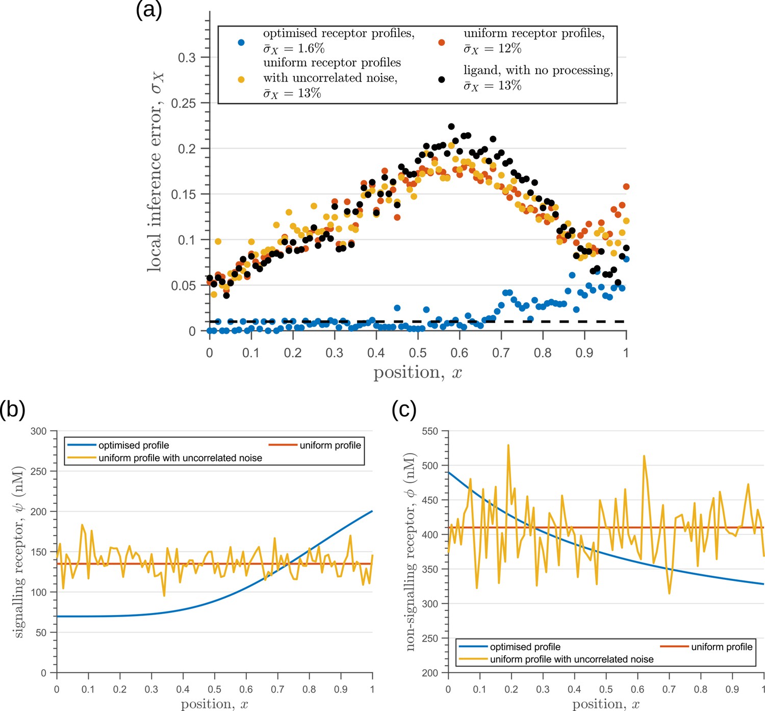
Behaviour of inference error on varying receptor profiles.

(a) Inference error profiles due to extrinsic noise in the optimised two-tier two-branch channels with optimal receptor profiles (blue), uniform receptor profiles (red) and uniform receptor profiles with uncorrelated noise (orange). Having uniform receptor profiles simply reflects the noise in the ligand input (black). (b) Signalling receptor profiles corresponding to the cases in (a). (c) Non-signalling receptor profiles corresponding to the cases in (a). In (**b,c**), the mean uniform receptor concentration is set to the mid point of the optimised receptor profile while the strength of the uncorrelated noise is 0.1 times the mean. The chemical rates, receptor profile parameters and feedback parameters for the optimised two-tier two-branch channel can be found in Table 2 under the column corresponding to $n_{T} = 2, n_{B} = 2, r_{-} = κ_{I}$ . The optimised chemical rates and feedback parameters for the two-tier two-branch channels with uniform receptors can be found in Table 3.

Appendix 12—figure 1

Download asset Open asset

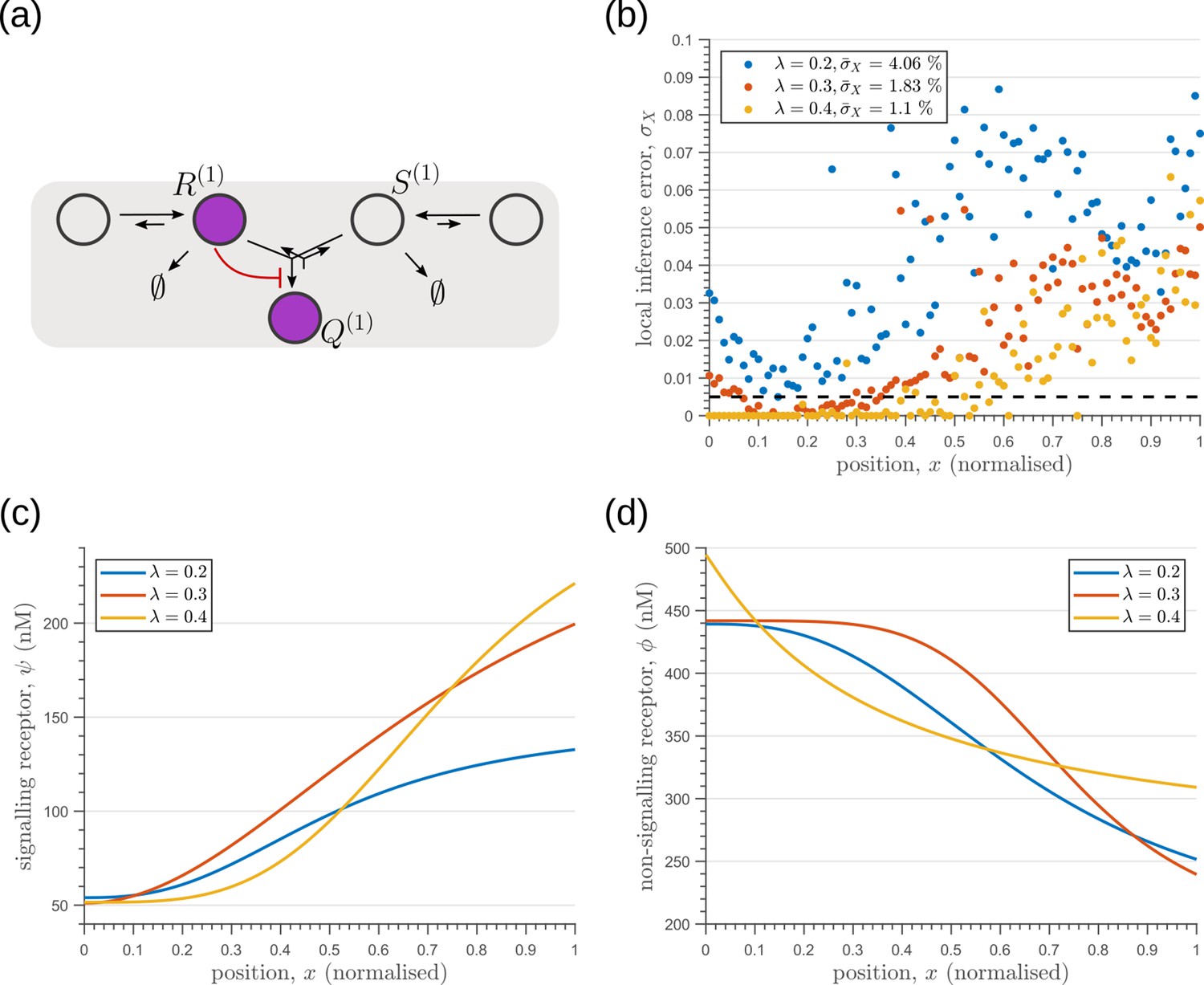
Optimisation of one-tier two-branch channels for extrinsic noise with varying mean input decay lengths $λ$ (Equation 2).

(a) The channel architecture with inter-branch feedback shows the lowest inference error for all values of $λ$ considered. (b) The minimum local and average inference errors decrease with $λ$ . (c) Optimised profiles of the signalling receptors are increasing functions of $x$ for the different values of $λ$ . (d) Optimised profiles of the non-signalling receptors are decreasing functions of $x$ for the different values of $λ$ .

Appendix 12—figure 2

Download asset Open asset

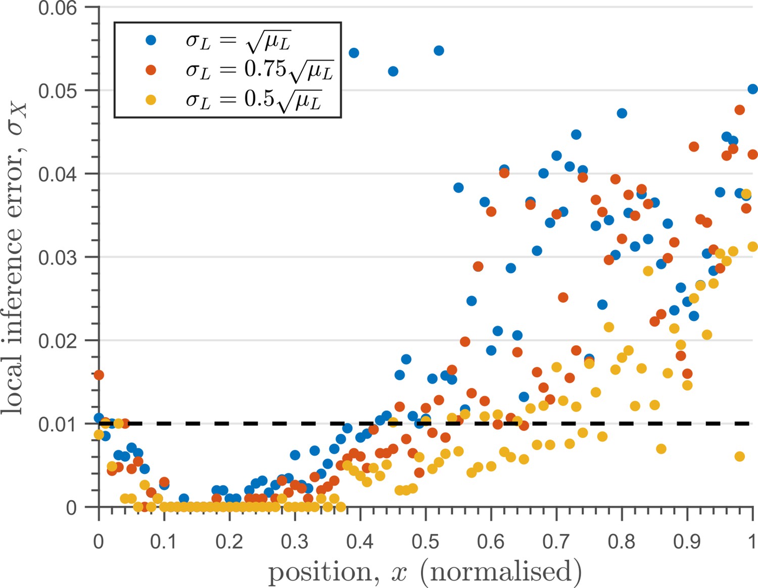
The one-tier two-branch channel optimised for ligand distribution with standard deviation equal to the square root of mean, $σ_{L} = \sqrt{μ_{L}}$ , and decay length $λ = 0.3$ shows smaller inference error for lower levels of input noise.

The dashed line corresponds to a local inference error of one cell’s width $\sim 1 / n_{x}$ . Note that the point at which local inference error departs away from 1% (one cell width error) extends further away from the source.

Appendix 13—figure 1

Download asset Open asset

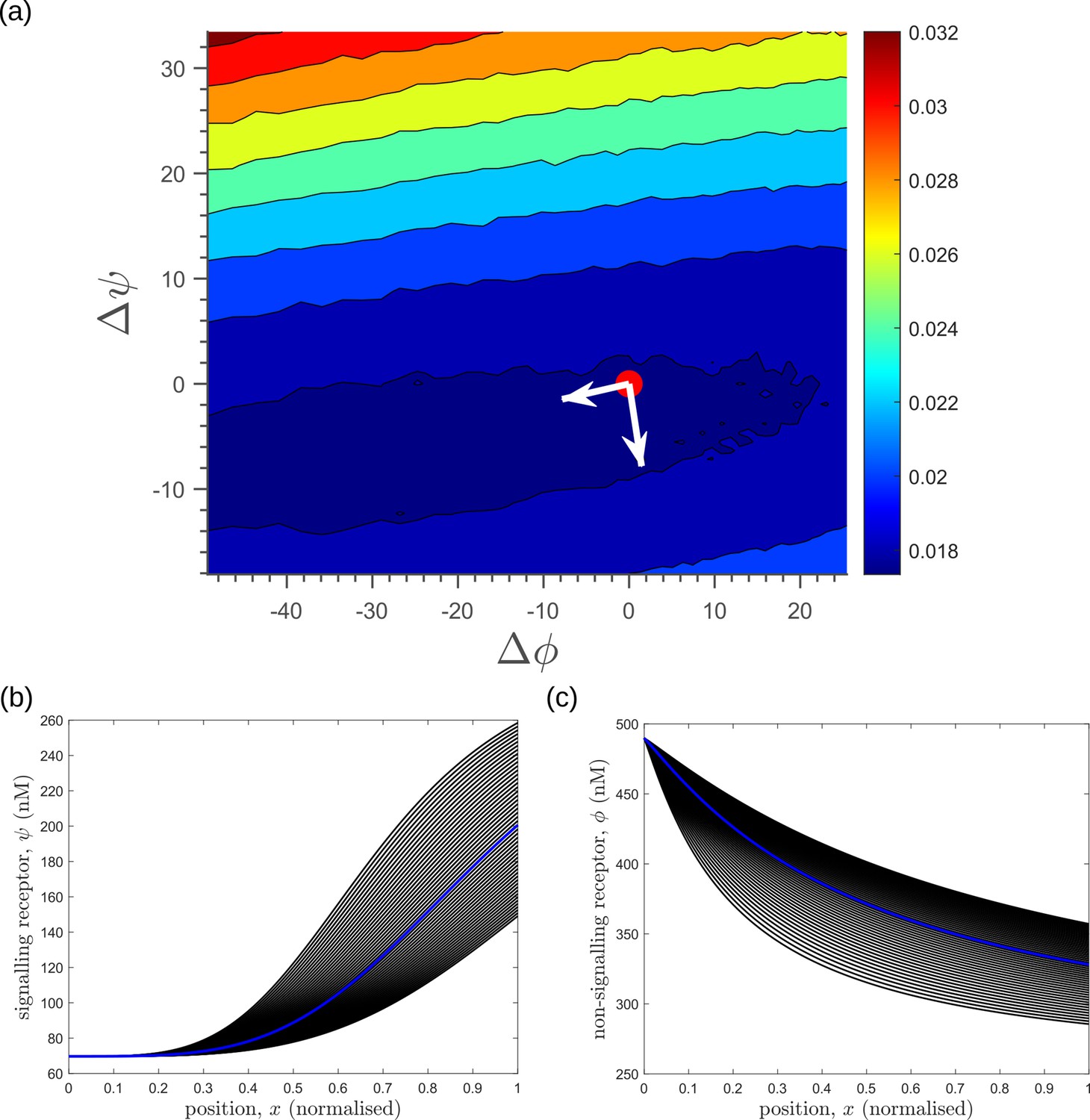
Response of average inference error in the optimised two-tier two-branch channel (Figure 8b of the main text) to changes in receptor profiles shows the *stiff-sloppy* directions of control on receptors.

(a) Contours of average inference error ${\bar{σ}}_{X}$ as functions of the net deviation from the optimal receptor profiles, as defined in Equations 45; 46. The white arrows indicate the directions of eigenvectors of the local Hessian (curvature) around the optimum (red point). The shorter arrow corresponds to the smaller eigenvalue (*sloppy* direction) while the longer arrow corresponds to the larger eigenvalue (*stiff* direction). (**b,c**) The allowed perturbations in receptor profiles, $ψ (x)$ and $ϕ (x)$ (black) around the optimal receptor profiles (blue), maintaining the nature of monotonicity. The optimised parameter values for the plots can be found in Table 2 under the column corresponding to $n_{T} = 2, n_{B} = 2, r_{-} = κ_{I}$ .

Appendix 14—figure 1

Download asset Open asset

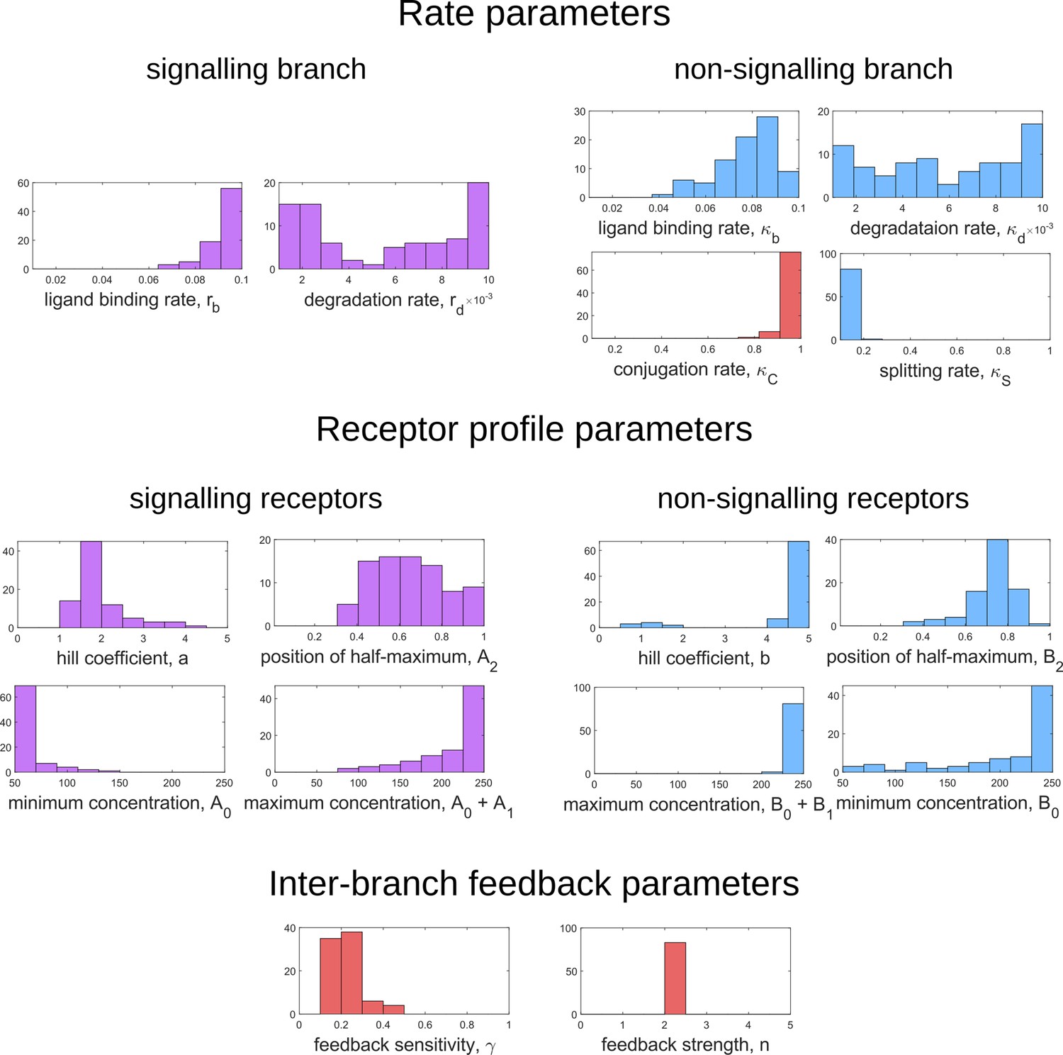
Frequency distributions of optimum channel parameters yielding ${\bar{σ}}_{X} \leq 2 %$ .

Symbols below each panel represent channel parameters listed in Table 1.

Tables

Table 1

Parameters associated with rates, feedback and receptor profiles along with their range of values.

The chemical rate values used in numerical analysis are scaled by the unbinding rate $r_{u}, κ_{u}$ taken to be 1. The corresponding experimental values have been taken from Lauffenburger and Linderman, 1996 where available.

Parameter	Symbol	Numerical values	Experimental values
Chemical rates
Signalling branch
Unbinding rate	r_u	1	0.34 ${min}^{- 1}$
Binding rate	r_b	0.1–1 ${nM}^{- 1}$	0.072 ${nM}^{- 1} {min}^{- 1}$
Degradation rate	r_d	0.001–0.01	0.0022 ${min}^{- 1}$
Internalisation rate	$r_{I}$	0.1–1	0.03–0.3 ${min}^{- 1}$
Recycling rate	$r_{R}$	0.1–1	0.058 ${min}^{- 1}$
Non-signalling branch
Unbinding rate	$κ_{u}$	1	-
Binding rate	$κ_{b}$	0.1–1 ${nM}^{- 1}$	-
Degradation rate	$κ_{d}$	0.001–0.01	-
Internalisation rate	$κ_{I}$	0.1–1	-
Recycling rate	$κ_{R}$	0.1–1	-
Conjugation rate	$κ_{C}$	0.1–1 ${nM}^{- 1}$	-
Splitting rate	$κ_{S}$	0.1–1	-
Feedback control
Amplification	$α$	$0.1 - 10$	-
Feedback Sensitivity	$γ$	$0 - 1$ ${nM}^{- 1}$	-
Feedback strength	n	$0 - 5$	-
Receptor control
Signalling receptors
Hill coefficient	$a$	$0 - 5$	-
Minimum concentration	A₀	$50 - 250$ nM	-
Maximum concentration	$A_{0} + A_{1}$	$50 - 500$ nM	-
Position of half-maximum	A₂	$0.01 - 1$	-
Non-signalling receptors
Hill coefficient	$b$	$0 - 5$
Minimum concentration	B₀	$50 - 250$ nM	-
Maximum concentration	$B_{0} + B_{1}$	$50 - 500$ nM	-
Position of half-maximum	B₂	$0.01 - 1$	-
Ligand input
Maximum concentration	$A$	30 nM	-
Decay length	$λ$	$0.2 - 0.5$	-
Number of cells along $x$ -direction	n_x	101	-
Number of cells along $y$ -direction	n_y	101	-

Table 2

Values of rates, feedback and receptor control parameters obtained after optimising the different channel architectures with $n_{T}$ tiers and $n_{B}$ branches.

The optimised values of the chemical rates quoted below are scaled by the unbinding rate r_u, $κ_{u}$ taken to be 1. The symbols $r_{-}$ and $r_{+}$ denote positive and negative feedbacks, respectively, on the rates following the equals sign; ${}$ implies absence of feedback.

Parameter (Symbol)	Value obtained in the optimised channel ( $n_{T}, n_{B}$ )
	(1,1)	(1,2)	(2,2)	(2,2)	(2,2)
	$r_{+} = r_{d}^{(1)}$	$r_{-} = κ_{C}$	$r_{-} = κ_{I}$	$r_{-} = κ_{C}$	$r_{-} = {}$
Chemical rates
Signalling branch
Binding rate ( $r_{b}, {nM}^{- 1}$ )	0.0898	0.0949	0.0932	0.0893	0.0787
Degradation rate in tier 1 ( $r_{d}^{(1)}$ )	0.0013	0.0081	0.0086	0.0098	0.0038
Degradation rate in tier 2 ( $r_{d}^{(2)}$ )	-	-	0.0066	0.0087	0.0016
Internalisation rate ( $r_{I}$ )	-	-	0.0531	0.0784	0.0363
Recycling rate ( $r_{R}$ )	-	-	0.0681	0.0359	0.0758
Non-signalling branch
Binding rate ( $κ_{b}, {nM}^{- 1}$ )	-	0.0590	0.0954	0.0835	0.0288
Degradation rate in tier 1 ( $κ_{d}^{(1)}$ )	-	0.0086	0.001	0.0043	0.0068
Degradation rate in tier 2 ( $κ_{d}^{(2)}$ )	-	-	0.0037	0.0031	0.0033
Internalisation rate ( $κ_{I}$ )	-	-	0.0741	0.0846	0.0559
Recycling rate ( $κ_{R}$ )	-	-	0.0123	0.0134	0.0998
Conjugation rate ( $κ_{C}, {nM}^{- 1}$ )	-	0.9926	0.9823	0.9722	0.6019
Splitting rate ( $κ_{S}$ )	-	0.1285	0.1545	0.1350	0.7512
Feedback control
Amplification ( $α$ )	3.2085	-	-	-	-
Feedback Sensitivity ( $γ$ )	0.2491	0.1831	0.5535	0.8259	-
Feedback strength ( $n$ )	2.6825	2.3683	2.0953	2.1880	-
Tier-wise weights
weight of tier 1 (w₁)	1	1	0.0018	0.1232	0.9259
weight of tier 2 (w₂)	-	-	0.9982	0.8768	0.0741
Receptor control
Signalling receptors
Hill coefficient ( $a$ )	4.9231	1.9974	3.8363	3.5251	3.3835
Minimum concentration ( $A_{0}, nM$ )	51.8130	51.0960	69.6940	51.9770	51.2
Maximum concentration ( $A_{0} + A_{1}, nM$ )	298.283	290.356	304.114	134	301
Position of half-maximum (A₂)	0.4752	0.7818	0.9405	0.8344	0.4091
Non-signalling receptors
Hill coefficient ( $b$ )	-	4.8951	1.0802	1.7472	3.1821
Minimum concentration ( $B_{0}, nM$ )	-	192.32	248.69	192.4	94.1850
Maximum concentration ( $B_{0} + B_{1}, nM$ )	-	442	489.77	441.67	305
Position of half-maximum (B₂)	-	0.7428	0.5177	0.3196	0.0902

Table 3

Values of chemical rates and feedback parameters obtained after optimising the two-tier two-branch channel with inter-branch feedback on the internalisation rate $κ_{I}$ of the non-signalling branch, keeping the receptor profiles spatially uniform, with and without uncorrelated noise.

The optimised values of the chemical rates quoted below are scaled by the unbinding rate r_u, $κ_{u}$ taken to be 1.

Parameter (Symbol)	Optimised value
Parameter (Symbol)	uniform receptor profiles	uniform receptor profiles with uncorrelated noise
Chemical rates
Signalling branch
Binding rate ( $r_{b}, {nM}^{- 1}$ )	0.0922	0.0782
Degradation rate in tier 1 ( $r_{d}^{(1)}$ )	0.0089	0.0041
Degradation rate in tier 2 ( $r_{d}^{(2)}$ )	0.0092	0.0095
Internalisation rate ( $r_{I}$ )	0.0225	0.0611
Recycling rate ( $r_{R}$ )	0.0403	0.0971
Non-signalling branch
Binding rate ( $κ_{b}, {nM}^{- 1}$ )	0.0464	0.0265
Degradation rate in tier 1 ( $κ_{d}^{(1)}$ )	0.0035	0.0045
Degradation rate in tier 2 ( $κ_{d}^{(2)}$ )	0.0071	0.0068
Internalisation rate ( $κ_{I}$ )	0.02	0.0513
Recycling rate ( $κ_{R}$ )	0.0989	0.0770
Conjugation rate ( $κ_{C}, {nM}^{- 1}$ )	0.7605	0.7579
Splitting rate ( $κ_{S}$ )	0.7038	0.3036
Feedback control
Amplification ( $α$ )	-	-
Feedback Sensitivity ( $γ$ )	0.0939	0.1946
Feedback strength ( $n$ )	4.6310	0.6202
Tier-wise weights
weight of tier 1 (w₁)	0.0046	0.2875
weight of tier 2 (w₂)	0.9954	0.7125

Additional files

MDAR checklist: https://cdn.elifesciences.org/articles/79257/elife-79257-mdarchecklist1-v1.pdf
Download elife-79257-mdarchecklist1-v1.pdf

Download links

A two-part list of links to download the article, or parts of the article, in various formats.

Downloads (link to download the article as PDF)

Open citations (links to open the citations from this article in various online reference manager services)

Mendeley

Cite this article (links to download the citations from this article in formats compatible with various reference manager tools)

Krishnan S Iyer
Chaitra Prabhakara
Satyajit Mayor
Madan Rao

(2023)

Cellular compartmentalisation and receptor promiscuity as a strategy for accurate and robust inference of position during morphogenesis

eLife 12:e79257.

https://doi.org/10.7554/eLife.79257

Share this article

Cite this article

Schematic of information processing in the developing tissue.

Schematic for the branch-tier channel architecture.

Family of receptor profiles fA (monotonically increasing in x) and fB (monotonically decreasing in x) with an interpretation of function parameters (Equations 8; 9).

Examples of channel architectures with single and multiple tiers, and upto two branches.

Schematic of feedback types.

Characteristics of an optimised (a) one-tier one-branch channel with only the signalling receptor and feedback.

Results of optimisation of (a) one-tier two-branch channel.

Performance of the optimised two-branch channels with increasing numbers of tiers.

Robustness to intrinsic noise in (a) one-tier two-branch (1T2B) channel and (b) two-tier two-branch (2T2B) channel architectures, previously optimised for extrinsic noise alone.

Geometry of the fidelity landscape around the optimum.

Geometry of the low inference error landscape defined by channels within a band σ¯X≤2% about the global minimum.

Robustness to extrinsic noise with a different choice of objective function (Equation 23) for one-tier one-branch channel (a–b), one-tier two-branch channel (c–d) and two-tier two-branch channel (e–f).

Robustness to intrinsic noise, with a different choice of objective function (Equation 23), in (a) one-tier two-branch (1T2B) channel and (b) two-tier two-branch (2T2B) channel architectures, previously optimised for extrinsic noise alone.

Comparison of theoretical results with experimental observations on Wg signalling system in Drosophila wing imaginal disc.

Figure 14—source data 1

Supporting measurements of fluorescence intensity profiles for Figure 14d and Figure 14f.

Figure 14—figure supplement 1—source data 1

Hill functions representing positive (left) and negative (right) feedback control on chemical rates r actuated by chemical species R.

Schematic of an ideal output profile.

Robustness-Sensitivity plots for nx-1=100 cohorts in the optimised channel architectures.

Contour plots of χ (see Eq.Equation 32) in the optimised one-tier two-branch channel with inter-branch feedback control (Figure 7a of the main text) showing the preferred receptor combinations (deep blue) for different values of mean input μL.

Contour plots of mean output ⟨θ⟩ in the optimised one-tier two-branch channel with inter-branch feedback control (Figure 7a of the main text).

Input-Output function of a minimal channel shows the importance of choosing the correct receptor profiles.

Concentrations of the signalling species R(1),Q(1) and total cellular output θ in the optimised one-tier two-branch channel with ψ=164⁢nM,ϕ=318⁢nM.

Results of optimisation of (a,d) two-tier two-branch channels.

Two- and three-species CRNs with production k1 and degradation k2 rates of species 1 (s1) and inter-conversion k3,k4 rates between the “signalling" (output generating) species (in purple box).

Phase portrait for Equation 43 with k0≫k1.

Results of optimisation of (a) two-tier two-branch channel with no feedback on rates.

Behaviour of inference error on varying receptor profiles.

Optimisation of one-tier two-branch channels for extrinsic noise with varying mean input decay lengths λ (Equation 2).

The one-tier two-branch channel optimised for ligand distribution with standard deviation equal to the square root of mean, σL=μL, and decay length λ=0.3 shows smaller inference error for lower levels of input noise.

Response of average inference error in the optimised two-tier two-branch channel (Figure 8b of the main text) to changes in receptor profiles shows the stiff-sloppy directions of control on receptors.

Frequency distributions of optimum channel parameters yielding σ¯X≤2%.

Parameters associated with rates, feedback and receptor profiles along with their range of values.

Values of rates, feedback and receptor control parameters obtained after optimising the different channel architectures with nT tiers and nB branches.

Values of chemical rates and feedback parameters obtained after optimising the two-tier two-branch channel with inter-branch feedback on the internalisation rate κI of the non-signalling branch, keeping the receptor profiles spatially uniform, with and without uncorrelated noise.

MDAR checklist

Downloads (link to download the article as PDF)

Open citations (links to open the citations from this article in various online reference manager services)

Cite this article (links to download the citations from this article in formats compatible with various reference manager tools)

Family of receptor profiles $f_{A}$ (monotonically increasing in $x$ ) and $f_{B}$ (monotonically decreasing in $x$ ) with an interpretation of function parameters (Equations 8; 9).

Geometry of the low inference error landscape defined by channels within a band ${\bar{σ}}_{X} \leq 2 %$ about the global minimum.

Hill functions representing positive (left) and negative (right) feedback control on chemical rates $r$ actuated by chemical species $R$ .

Robustness-Sensitivity plots for $n_{x} - 1 = 100$ cohorts in the optimised channel architectures.

Contour plots of $χ$ (see Eq.Equation 32) in the optimised one-tier two-branch channel with inter-branch feedback control (Figure 7a of the main text) showing the preferred receptor combinations (deep blue) for different values of mean input $μ_{L}$ .

Contour plots of mean output $⟨ θ ⟩$ in the optimised one-tier two-branch channel with inter-branch feedback control (Figure 7a of the main text).

Concentrations of the signalling species $R^{(1)}, Q^{(1)}$ and total cellular output $θ$ in the optimised one-tier two-branch channel with $ψ = 164 nM, ϕ = 318 nM$ .

Two- and three-species CRNs with production k₁ and degradation k₂ rates of species 1 (s₁) and inter-conversion $k_{3}, k_{4}$ rates between the “signalling" (output generating) species (in purple box).

Phase portrait for Equation 43 with $k_{0} ≫ k_{1}$ .

Optimisation of one-tier two-branch channels for extrinsic noise with varying mean input decay lengths $λ$ (Equation 2).

The one-tier two-branch channel optimised for ligand distribution with standard deviation equal to the square root of mean, $σ_{L} = \sqrt{μ_{L}}$ , and decay length $λ = 0.3$ shows smaller inference error for lower levels of input noise.

Frequency distributions of optimum channel parameters yielding ${\bar{σ}}_{X} \leq 2 %$ .

Values of rates, feedback and receptor control parameters obtained after optimising the different channel architectures with $n_{T}$ tiers and $n_{B}$ branches.

Values of chemical rates and feedback parameters obtained after optimising the two-tier two-branch channel with inter-branch feedback on the internalisation rate $κ_{I}$ of the non-signalling branch, keeping the receptor profiles spatially uniform, with and without uncorrelated noise.