Sequential addition of neuronal stem cell temporal cohorts generates a feed-forward circuit in the Drosophila larval nerve cord
- Department of Molecular Genetics and Cell Biology, University of Chicago, United States
- Committee on Computational Neuroscience, University of Chicago, United States
- Program in Cell and Molecular Biology, University of Chicago, United States
- Committee on Neurobiology, University of Chicago, United States
- Department of Neurobiology, University of Chicago, United States
- University of Chicago Neuroscience Institute, United States
Figures
Figure 1 with 1 supplement
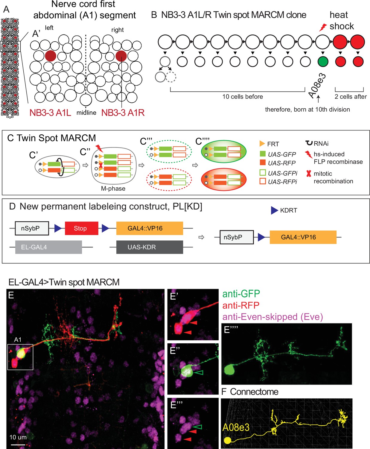
Twin-spot mosaic analysis with a repressible cell marker (ts-MARCM) determines the birth order and morphology of NB3-3A1L/R neurons.
(A, B) Illustrations of Drosophila neuroblasts. (A) The nerve cord is left–right symmetrical and segmented. Each circle represents one neuroblast with NB3-3 in maroon. Segment A1 (boxed) is enlarged in (A’). It contains 30 types of neuroblasts. (B) NB3-3 lineage progression is shown with an example ts-MARCM clone overlaid. Each circle represents one cell and each arrow represents a cell division. First, NB3-3 divides to self-renew and generate a ganglion mother cell, which divides to generate a motor neuron (solid circle) and an undifferentiated cell (dashed circle). Then, NB3-3 directly generates ELs. In ts-MARCM, a heat shock is provided (red lightning bolt) as NB3-3 divides. In this example, a singly labeled neuron is shown in green (A08e3), and two alternatively labeled neurons are shown in red. Because the total number of neurons in the lineage is known, counting labeled neurons allows inference of neuronal birth order. The identity of the singly labeled neuron is determined by matching the labeled neuron to the corresponding neuron in the connectome using morphological criteria (see ‘Materials and methods’). (C, D) Illustration of ts-MARCM genetic constructs used in this study. Our updated version of ts-MARCM system has four components (C, D). (1) It uses a pair of genetically modified chromosomes. On one chromosome is an FRT recombinase site (yellow triangle) followed by a UAS-GFP (solid green box) and a UAS-RFP-RNAi (hollow red box) construct. On the other chromosome is an FRT site followed by a UAS-RFP (solid red box) and a UAS-GFP-RNAi (hollow green box) construct. When cells are heterozygous for these chromosomes, the GFP- and RFP- RNAi constructs ensure repression of GFP and RFP protein expression, respectively (black curves, C’). (2) It has a heat-shock-inducible FLP recombinase (red lightning bolt). By varying the heat shock protocol, we control both the timing and amount of FLP supplied. Heat shocks induce FRT-based chromosomal recombination in dividing cells (red X, M-phase cell, C’’). A subset of recombination events produce a pair of post-mitotic progeny, one of which is homozygous for the UAS-GFP, UAS-RFP-RNAi construct, and the other homozygous for the UAS-RFP, UAS-GFP-RNAi construct. In these cells, RNAi is no longer able to repress GFP or RFP expression (C’’’). (3) A cell-type-specific GAL4 line, (e.g., EL-GAL4, light gray box in B) is used to drive expression of UAS-RFP or UAS-GFP (C’’’’). (4) To get robust ts-MARCM labeling in early-stage larvae, it was often necessary to amplify GAL4 expression. To do so, we generated a new permanent labeling construct (D). Specifically, a neuron-specific nSyb promoter (white box) is upstream of a Stop (red box) flanked by KDRT (blue triangles) recombination sights. When the KDR recombinase (from UAS-KD, dark gay box) is supplied, the Stop is removed, and nSyb drives expression of a the new GAL4 (yellow box). This new GAL4 is the GAL4 DNA binding domain tethered to the strong transcriptional activator VP16. (E, F) Image of a ts-MARCM clone and a corresponding neuron in the connectome. (E) Many segments of the nerve cord are shown in dorsal view with anterior up. The boxed region in segment A1 is enlarged at the right. In this ts-MARCM clone, two neurons are labeled in red and one in green (arrowheads), and all are Eve(+) ELs. The singly labeled EL is enlarged to highlight morphological detail. The corresponding neuron in the connectome is shown in (F). Specific genotype is listed in Supplementary file 4.
Figure 1—figure supplement 1
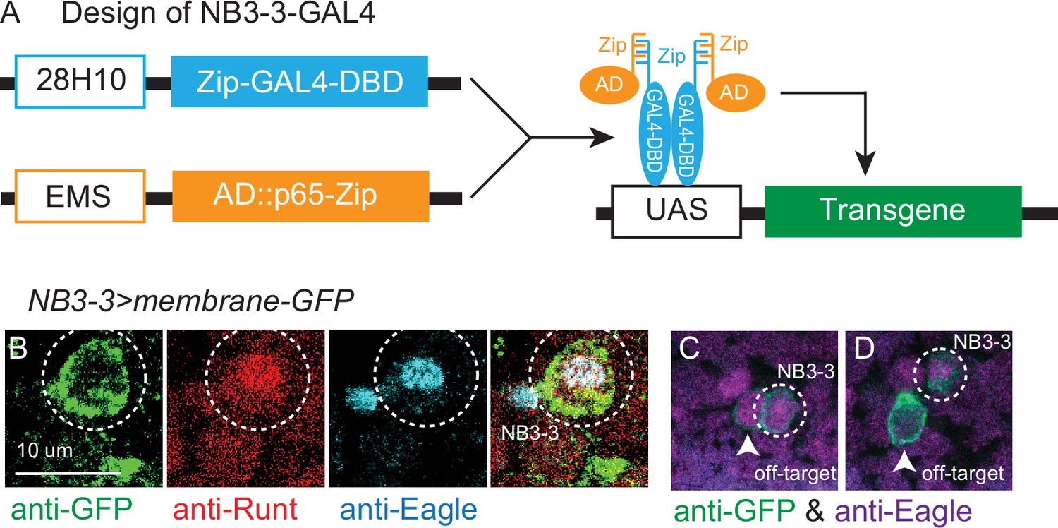
NB3-3-GAL4 line.
(A) Illustration of NB3-3-GAL4 line. 28H10 (blue outlined box) and EMS (orange outlined box) are promoters that drive in different subsets of neuroblasts, whose expression overlaps specifically in NB3-3. Zip-GAL4-DBD encodes the DNA binding domain of the yeast transcription factor GAL4 (blue box). It binds the yeast UAS promoter. AD-Zip encodes an activation domain peptide that recruits transcriptional machinery to a promoter (orange box). When Zip-GAL4-DBD and AD-Zip are expressed in the same cell, they activate expression of any transgene downstream of UAS promoter (green box). See ‘Materials and methods’ for construction of EMS-zp-AD. (B, C, D) Images of NB3-3-GAL4 expression. (B) NB3-3-GAL4 labels NB3-3, which is selectively labeled by the overlap in expression of Runt (red) and Eagle (cyan). Dashed circle shows NB3-3. (C, D) NB3-3-GAL4 expresses in NB3-3 as well as a few, variable other neuroblasts. Eagle (magenta) labels four neuroblasts (NB3-3, NB6-4, NB2-4, NB7-3). Arrows point to NB-3 ‘off-target’ cells, dashed circles show a bone fide NB3-3. Single optical slices of stage 11 embryos are shown in dorsal view with anterior up NB3-3-GAL4 (dashed circle) drives membrane GFP. For genotype, see Supplementary file 4.
Figure 2
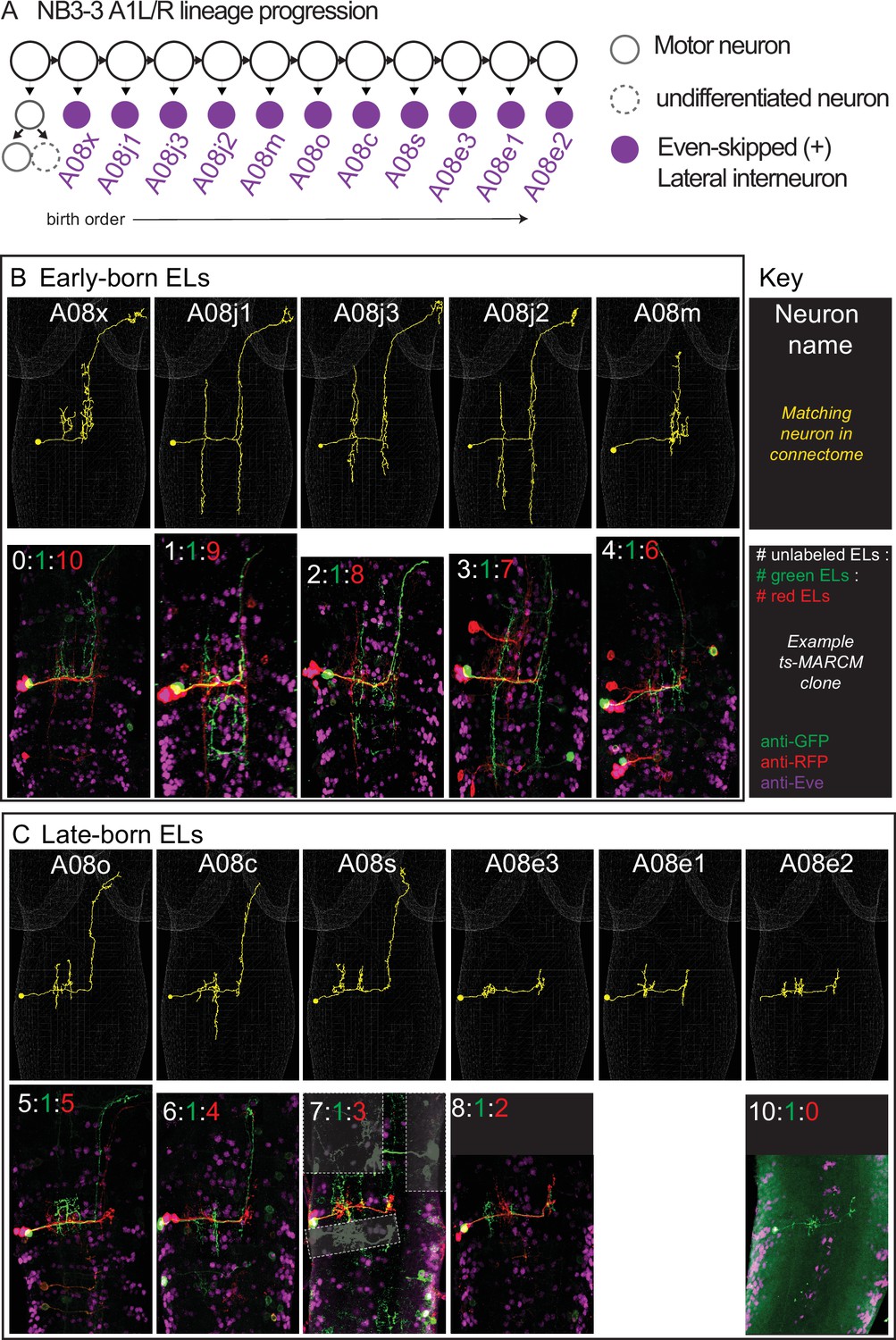
Twin-spot mosaic analysis with a repressible cell marker (ts-MARCM) provides birth order for all neurons in the NB3-3A1L/R lineage.
(A) Schematic of NB3-3A1 lineage progression is shown with EL birth order. Each circle represents one cell, and each arrow represents a cell division. (B, C) Images of individually labeled ts-MARCM clones shown in birth order. Early-born ELs are show in the top box, and late-born ELs are shown in the bottom. An image key is shown to the right of the early-born ELs. Briefly, all images are shown in a dorsal view with anterior to the top. The neuron name is at the top of each image pair, along with an example of the neuron in the connectome (yellow). The bottom of each image pair is an example of a clone stained with anti-GFP, anti-RFP, and anti-Eve. At the top of the example clone image is the number of unlabeled ELs (white), the number of ELs labeled in green, and the number of ELs labeled in red. Sometimes clones in other segments are lightly boxed over for clarity. For genotype, see Supplementary file 4.
Figure 3
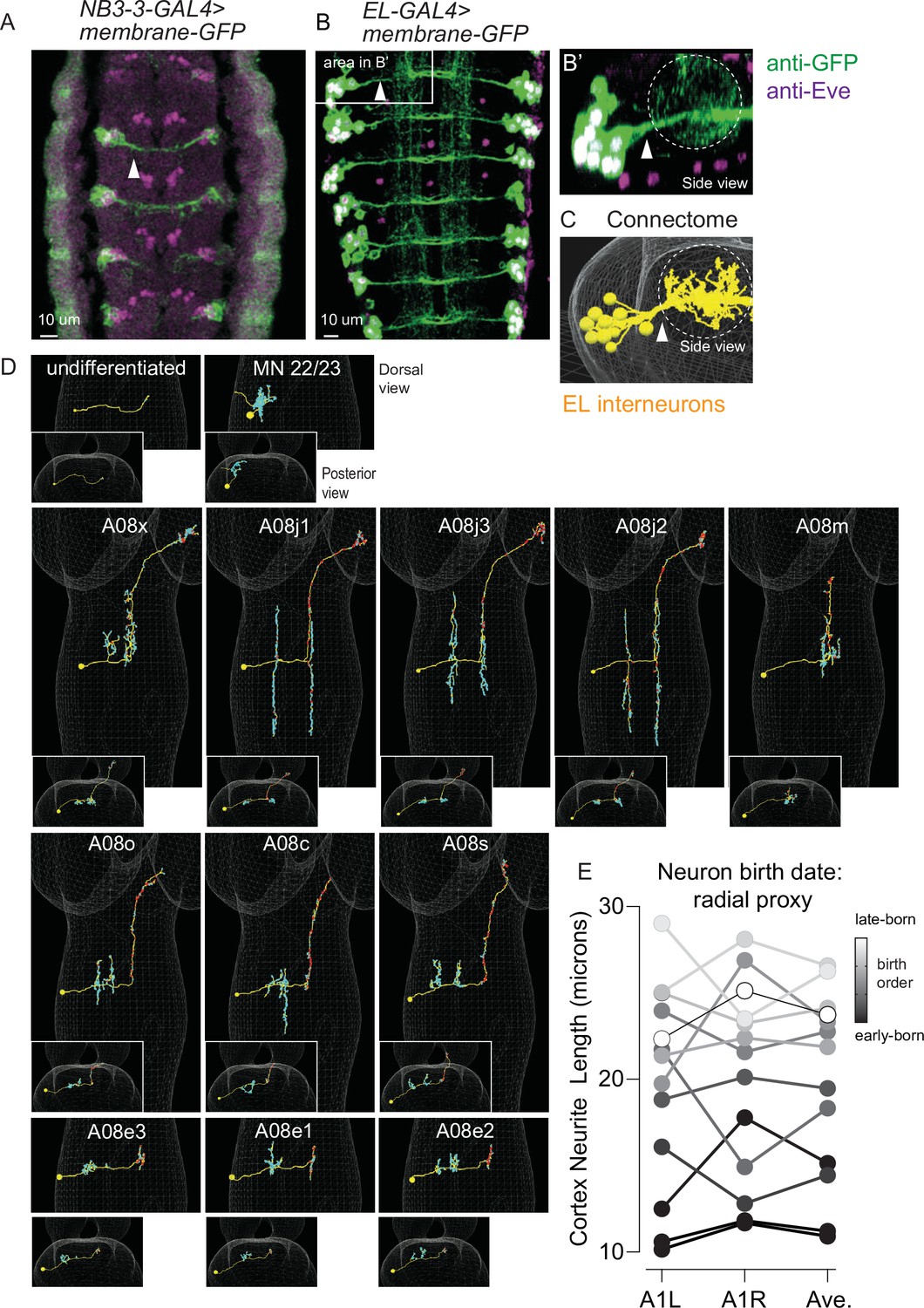
The morphology of all NB3-3A1L/R neurons in the connectome.
(A–C) Images of NB3-3A1L neurons with clustered soma and bundled neuritis. (A, B) NB3-3-GAL4 or EL-GAL4 driving expression of membrane GFP was immortalized using a permanent labeling strategy (Supplementary file 4). Arrowheads point to bundles formed by neurons before they enter the neuropil. The images are dorsal views with anterior up. In (A), a stage 12 embryo, all NB3-3 neuronal progeny (including two non-ELs) are in a bundle. In (B), a first instar larva shows that in larval stages ELs form a bundle. The box shows segment A1L, which is enlarged and rotated in (B’). (B’) shows a posterior view of the bundle as it enters the neuropil (dashes). An image corresponding to (B’) from the connectome is shown in (C). (D) Images of each NB3-3A1L neuron in the connectome with synapse locations. For each image, a faint white mesh shows the outline of central nervous system (CNS) volume. Large images are dorsal views with anterior up. Smaller images are posterior views (looking towards the brain) with dorsal up. Yellow circles and lines are soma and neurites, respectively. Red and cyan dots are pre- and postsynaptic specializations, respectively. Neuron names are shown at the top of each panel. First-born NB3-3A1L/R progeny are in the top row; early-born ELs in the middle row; and late-born ELs in the bottom two rows. (E) Quantification of NB3-3A1L/R cortex neurite length as a proxy for birth timing. The length of the neurites between the soma and neuropil has been used as a proxy for neuronal birth timing. Plotted on the y-axis are cortex neurite lengths computed for NB3-3 neurons in segment A1L, A1R, and their average. Each dot represents a single neuron (or average of two). Gray scale shows the precise birth order as determined by twin-spot mosaic analysis with a repressible cell marker (ts-MARCM). There is a rough correlation between birth order and neurite length, with earlier-born neurons possessing shorter neurites.
-
Figure 3—source data 1
NB3-3A1L/R cortex neurite length.
- https://cdn.elifesciences.org/articles/79276/elife-79276-fig3-data1-v2.xlsx
Figure 4
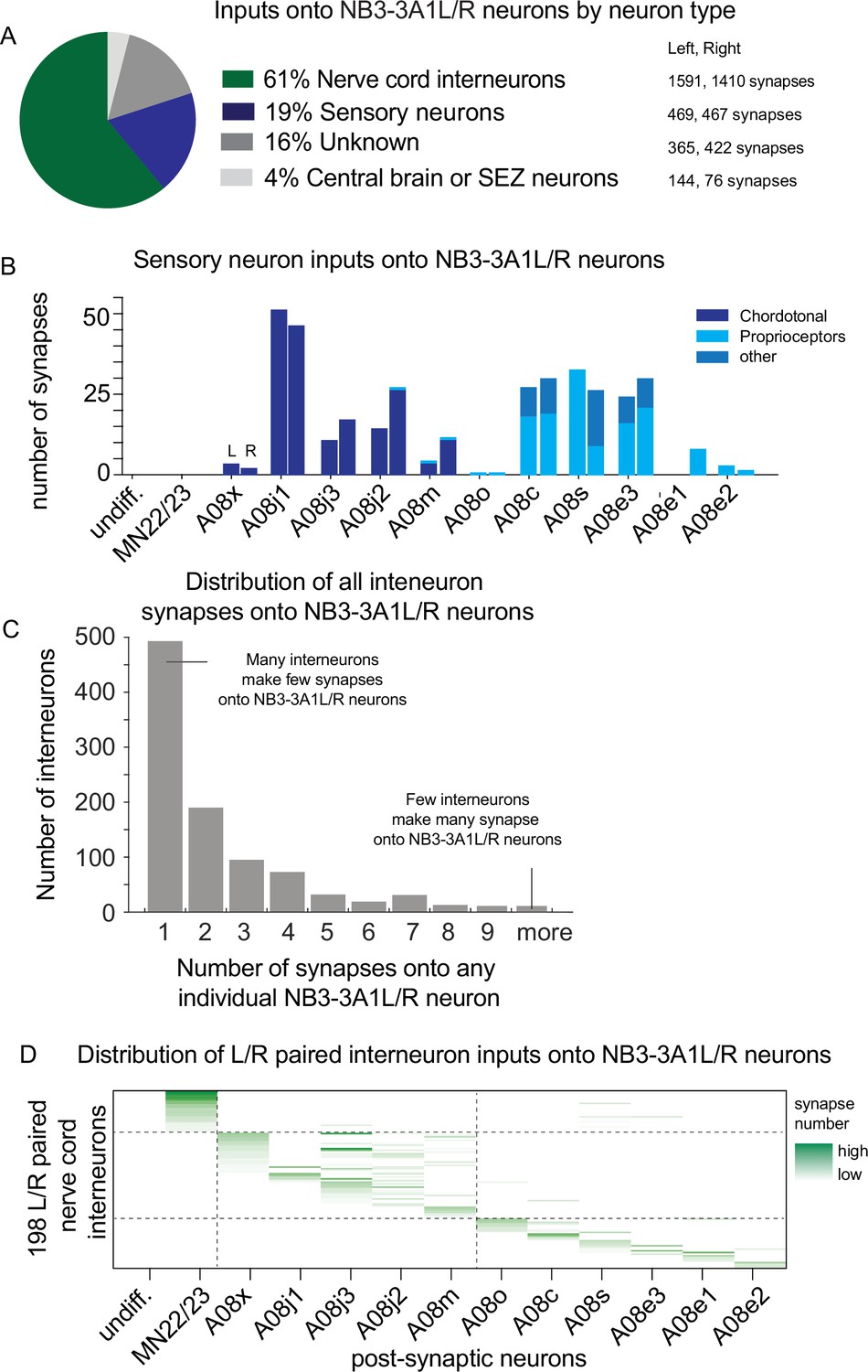
There are sharp transitions in lineage progression with respect to sensory neuron and interneuron inputs onto NB3-3A1L/R.
(A–D) Quantification of synaptic inputs onto NB3-3A1L/R. (A) The pie chart displays the percentage of total synapses from a given neuron type onto NB3-3A1L neurons. Data are color-coded, and the total number of synapses contributed by a given neuron type is shown at right. (B) Sensory neurons form synapses onto NB3-3A1L/R neurons. Chordotonal sensory neurons (dark blue) synapse onto early-born ELs. Late-born ELs get input from proprioceptive or other sensory neurons (lighter blues). The Y-axis represents the proportion of total synaptic input onto a given neuron that come from a single class of sensory neuron. Columns in the X-axis represent pairs of postsynaptic NB3-3A1L (L) and NB3-3A1R (R) neurons sorted by birth order. (C) Many individual nerve cord interneurons synapse onto NB3-3A1L/R neurons only a few times, whereas few individual nerve cord interneurons provide multiple synapses onto NB3-3A1L/R neurons. The X-axis shows histogram bins representing number of synapses contributed to an individual neuron. The Y-axis represents the number of individual nerve cord interneurons in each bin. (D) Distribution of major interneuron inputs onto NB3-3A1L/R neurons. The Y-axis represents 198 left right (L/R) paired nerve cord interneurons (see ‘Materials and methods’). Each column represents one neuron. Names are not shown due to space limitations. Columns in the X-axis represent postsynaptic NB3-3A1L/R neurons. If an input interneuron forms a synapse with a NB3-3A1L/R neuron, the row–column intersection is shaded green, with darker the green representing greater number of synapses. Dashed lines are placed at the border between non-ELs, early-born ELs, and late-born ELs.
-
Figure 4—source data 1
All synaptic input neuron information onto NB3-3A1L/R.
- https://cdn.elifesciences.org/articles/79276/elife-79276-fig4-data1-v2.xlsx
-
Figure 4—source data 2
Sensory input onto NB3-3A1L/R neurons.
- https://cdn.elifesciences.org/articles/79276/elife-79276-fig4-data2-v2.xlsx
-
Figure 4—source data 3
Summary of NB3-3A1L/R input neurons based on number of input.
- https://cdn.elifesciences.org/articles/79276/elife-79276-fig4-data3-v2.xlsx
-
Figure 4—source data 4
NB3-3A1L/R input from L/R paired neurons.
- https://cdn.elifesciences.org/articles/79276/elife-79276-fig4-data4-v2.xlsx
Figure 5
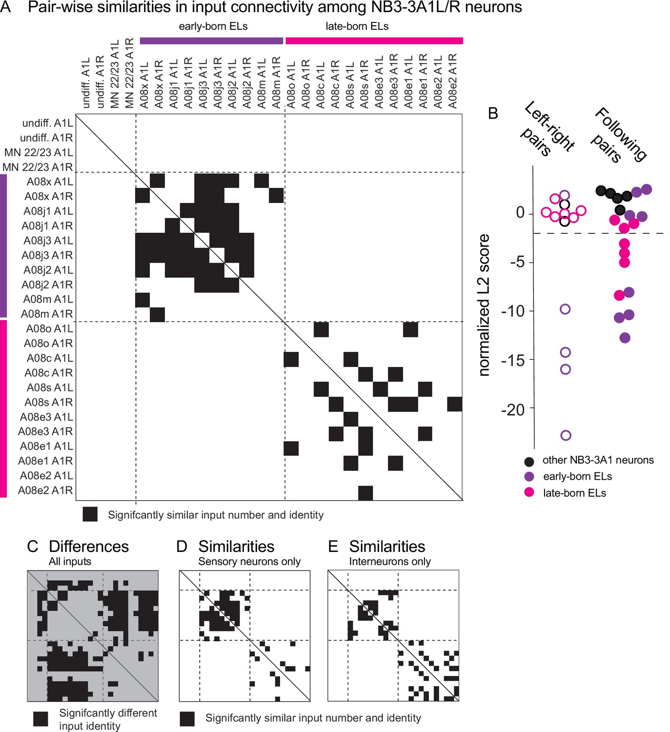
Early-born and late-born ELs have significantly similar input connectivity patterns between different temporal cohorts.
(A–E) Quantifications of input connectivity between NB3-3A1L/R neurons using network analysis. (A) The plot shows pairwise comparisons of input connectivity with significant similarities in black (normalized, nonbinary distance analysis, see ‘Materials and methods’). The plot is symmetric, and a solid line shows the diagonal. Left and right NB3-3A1 neurons are arranged in order of their birth on the X-axis and Y-axis. Early-born ELs are indicated with purple and late-born ELs with magenta. Row–column pairs with scores significantly smaller than shuffled controls are shown in black (p<0.05). Dashed lines are placed at the border between non-ELs, early-born ELs, and late-born ELs. (B) The plot shows a summary of pairwise differences in input connectivity (normalized, binary distance analysis, see ‘Materials and methods’). At left is a comparison of left–right neuron pairs of the same neuron (hollow circles) and at right is a comparison of two neurons that follow each other birth order (solid circles). All left–right pairs with significant similarities are early-born ELs. Both early-born and late-born ELs have significant similarities between following pairs. Significance threshold (p<0.05) is marked in a dashed line. Smaller scores indicate increased input similarity. (C) The plot is similar to that in (A), but shows normalized Euclidean distance differences between neuron pairs. The background is gray to visually distinguish it from similarity plots. Black area indicates pairs whose input identities are significantly different than would be expected by chance (p<0.05). (D, E) The plots are similar to that in (A), but computed separately with sensory neuron-only or interneuron-only inputs.
-
Figure 5—source data 1
z-scores for similarity.
- https://cdn.elifesciences.org/articles/79276/elife-79276-fig5-data1-v2.xlsx
-
Figure 5—source data 2
z-scores for differences.
- https://cdn.elifesciences.org/articles/79276/elife-79276-fig5-data2-v2.xlsx
-
Figure 5—source data 3
Similarity z-scores for sensory only input.
- https://cdn.elifesciences.org/articles/79276/elife-79276-fig5-data3-v2.xlsx
-
Figure 5—source data 4
Similarity z-scores for interneuron only input.
- https://cdn.elifesciences.org/articles/79276/elife-79276-fig5-data4-v2.xlsx
Figure 6
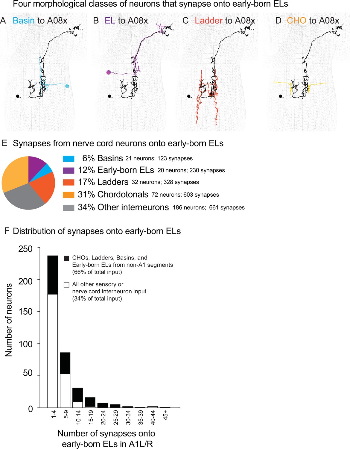
At the population level and single-neuron level, four morphological classes of neurons provide the majority of synaptic input onto early-born ELs in A1.
(A–D) Images of neurons from each class. Examples of neuron morphology from connectome data. Black mesh shows the outline of the central nervous system (CNS), anterior is up, images show in dorsal view. The early-born EL, A08x A1L, is shown in black. The other neurons with inputs onto A08x are shown in color code in (E). CHO, chordotonal sensory neuron. (E, F) Quantification of nerve cord synapses onto early-born ELs. (E) The pie chart displays inputs onto early-born ELs as a proportion of total population of inputs. Each slice is the percentage of synapses from a given anatomical class (e.g., Ladders) compared to the nerve cord neuron synapses (Supplementary file 2). (F) A stacked histogram shows the distribution of synaptic contacts made by individual neurons. Black shows the group of neurons that includes in CHO, Ladder, Basin, and early-born ELs from segments other than A1 (black). White shows a group containing all other neurons. The X-axis are histogram bins representing a range of synapse numbers contributed to all early-born ELs in segment A1. The Y-axis represents the number of individual nerve cord interneurons in each bin.
-
Figure 6—source data 1
Basin, EL, Ladder, and CHO input onto early-born ELs in A1L/R.
- https://cdn.elifesciences.org/articles/79276/elife-79276-fig6-data1-v2.xlsx
-
Figure 6—source data 2
Distribution of input onto early-born ELs in A1L/R.
- https://cdn.elifesciences.org/articles/79276/elife-79276-fig6-data2-v2.xlsx
Figure 7
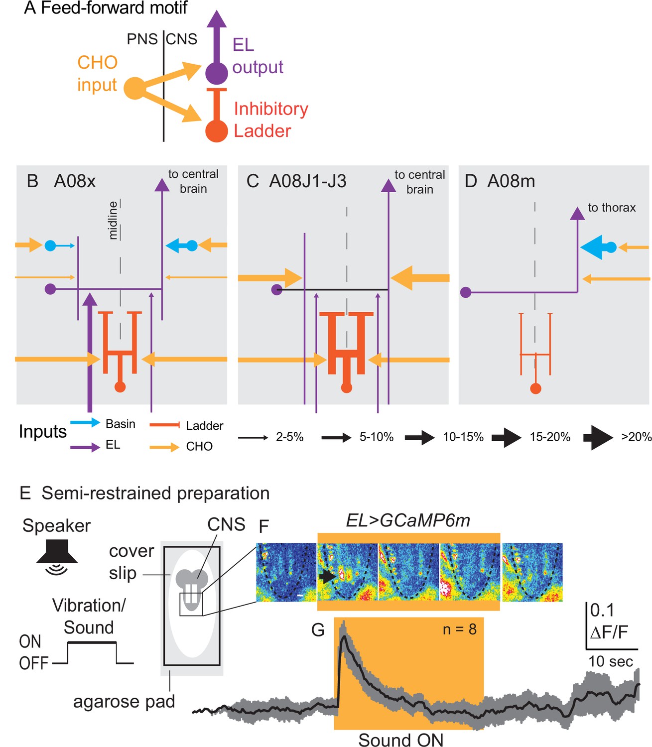
Early-born ELs are embedded in a feed-forward motif and encode the onset of vibrational stimuli.
(A–D) Illustrations of patterns of synaptic inputs onto early-born ELs. (A) A simplified schematic show the feed-forward motif in which early-born ELs are embedded. (B–D) Schematics of patterns of synaptic inputs onto different early-born ELs. Arrows are excitatory connections and bars are inhibitory (i.e., Ladders). The key at bottom shows how line thickness corresponds to percentage of inputs onto a given neuron. (E) Illustration of the preparation and stimulus protocol used for calcium imaging. A larva is placed on a bed of agarose with a cover slip on top. Fluorescence in the central nervous system (CNS) (gray lobed structure with two white lines [neuropil]) is recorded before, during, and after a sound is played from a speaker. (F) Images from representative recordings of calcium signals in ELs. Frames from a representative recording are shown at 8 s intervals. Yellow box indicates frames where sound stimulus was ON. Images are pseudo-colored with white/red as high fluorescence intensity and blue as low. Anterior is up. Scale bar is 50 µm. Dashed lines show the outline of the nerve cord. The black arrow in the second image panel indicates a region of neuropil with increased fluorescence. (G) Quantifications of EL calcium signals. Changes in EL calcium signaling upon vibrational stimulus (yellow box) show a rapid increase followed by decay. The black line represents average fluorescence intensity and gray represents standard deviation. ΔF/F is the change in fluorescence over baseline. N = number of larvae recorded. For genotype, see Supplementary file 4.
-
Figure 7—source data 1
Breakdown of Basin, EL, Ladder, and CHO input onto individual early-born ELs.
- https://cdn.elifesciences.org/articles/79276/elife-79276-fig7-data1-v2.xlsx
Figure 8
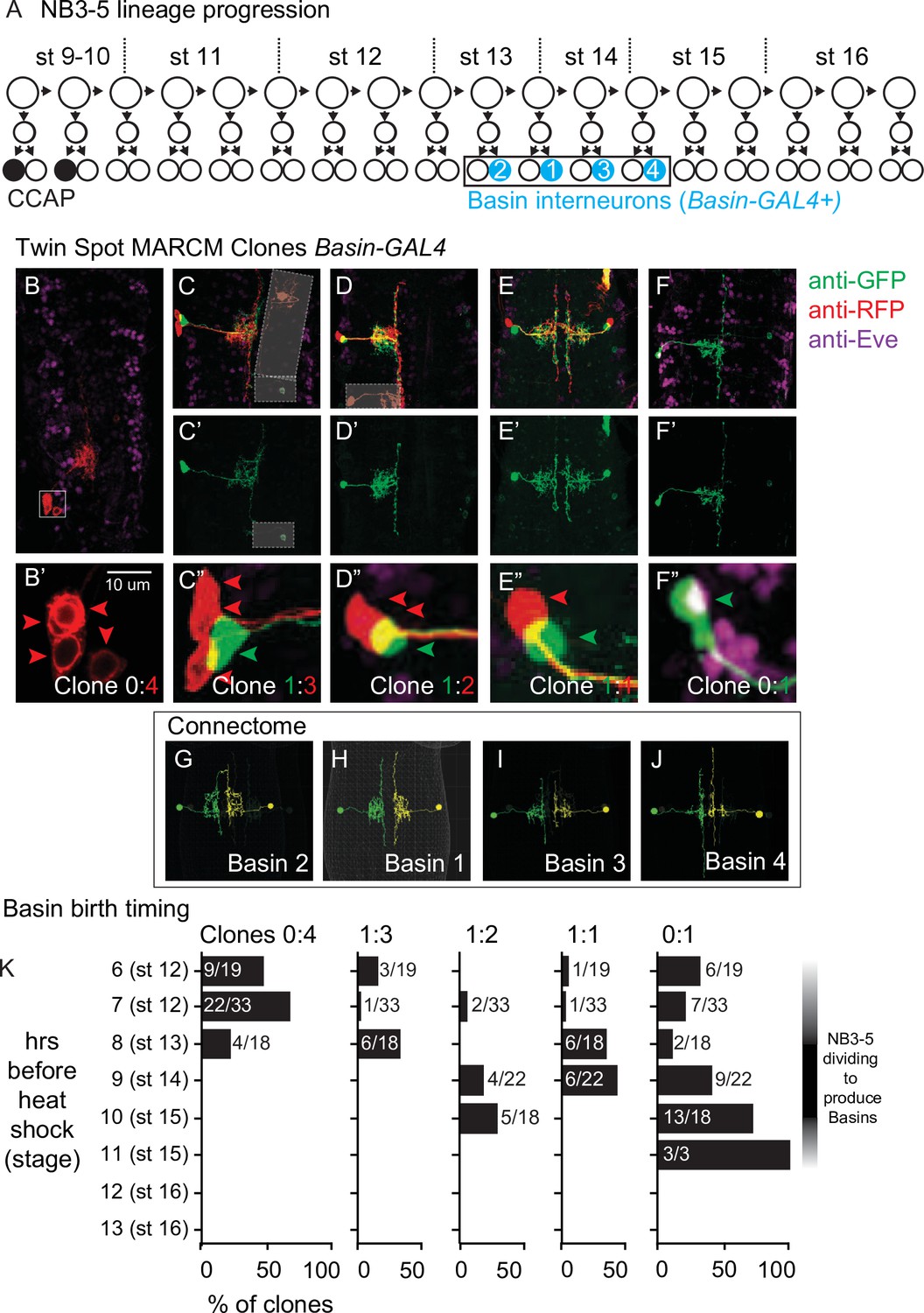
Birth time and birth order of Basin interneurons using twin-spot mosaic analysis with a repressible cell marker (ts-MARCM).
(A) Illustration of NB3-5 lineage progression. Each circle represents one cell, and each arrow represents a cell division. The X-axis represents developmental time, and dashes represent approximate positions of embryonic stages (e.g., st16). NB3-5 generates two CCAP(+) neurons (black) followed by a series of other neurons. Basins (cyan) are born a middle-to-late window. (B–J) Images of Basin ts-MARCM clones and Basins in the connectome. Examples of ts-MARCM clones are shown in (B–F’). Eve staining serves as a counterstain to visualize the nerve cord architecture. RFP and GFP show ts-MARCM Basin clones. Genotype in Supplementary file 4. (B) shows an example of a clone produced by an early, brief heat shock (see ‘Materials and methods’). In this nerve cord, only one clone is present, and in that clone, all four Basins are labeled. (B’) corresponds to the boxed region in (B). Red arrowheads point to each cell body (two are stacked on each other). (C–F”) show examples of other clone types. (C–F) shows two color labeling. (C’–F’) show morphology of the singly labeled Basin. (C”–F”) show higher magnification of the cell bodies with arrowheads pointing to labeled cells. Clone types indicated at the bottom of the panel. In (C), boxes with white dashes have been placed over ‘off target’ clones for visual clarity. (G–J) show left–right pairs of Basin interneurons in segment A1 of the connectome. All images shown in dorsal view with anterior up. (K) Quantification of types of clones produced by variously timed heat shocks. The clone type is displayed at the top of each graph. Y-axis for each graph shows the various times after egg collection until heat shock was applied. The X-axis for each graph represents the percentage of clones of that clone type that were produced by a given heat shock protocol. Numbers are the total number of clones of a clone type over the total number of clones scored for that time point.
Figure 9
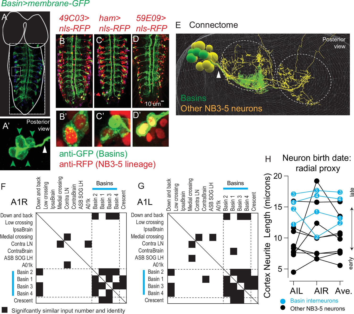
Basins are a middle-to-late-born temporal cohort in the NB3-5 lineage.
(A–E) Images of Basin interneurons and other lineage-related neurons. (A) The larval central nervous system (CNS) with Basins neurons expressing membrane GFP is shown in dorsal view with anterior up. For context, the outline of the nerve cord and brain lobes is shown in white. Dashed box outlines the image. The small light box region is shown in (A’). The green arrowheads point to Basin cell bodies, which are clustered. The white arrow points to bundle of Basin neurites. (B–D’) Larval nerve cords show co-expression of a Basin marker (membrane GFP) and various NB3-5 progeny markers (nuclear localized RFP). Genotypes in Supplementary file 4. (E) An image of NB3-5 progeny in the connectome is shown. The neuropil is outlined by dashed circles. Basin neurons are in green, and other neurons in the NB3-5 lineage are in yellow. Arrowhead points to the bundle containing Basins. (F–H) Quantification of Basin features using connectome data. (F, G) To quantify the similarity in wiring between neurons in the NB3-5 lineage, normalized (nonbinary) distance plots were generated. Right and left NB3-5A1 neurons are arranged in approximate order of their birth (based on average cortex neurite length) with Basins indicated by cyan bars. Row–column pairs with scores significantly smaller than shuffled controls are in black (p<0.05). The distance analysis plot is symmetric (solid line for the diagonal). Dashed lines are placed at the border between Basins and non-Basins. (H) The approximate birth order of Basins within the NB3-5 lineage was determined using cortex neurite length as a proxy. The Y-axis plots cortex neurite lengths for NB3-5 neurons in segment A1L, A1R, and their average. Compared to other neurons in the NB3-5 lineage, Basins are born near the end of the lineage.
-
Figure 9—source data 1
NB3-5 input neuron information.
- https://cdn.elifesciences.org/articles/79276/elife-79276-fig9-data1-v2.xlsx
-
Figure 9—source data 2
Similarity z-score for NB3-5 A1R.
- https://cdn.elifesciences.org/articles/79276/elife-79276-fig9-data2-v2.xlsx
-
Figure 9—source data 3
Similarity z-score for NB3-5 A1L.
- https://cdn.elifesciences.org/articles/79276/elife-79276-fig9-data3-v2.xlsx
-
Figure 9—source data 4
NB3-5 cortex neurite length.
- https://cdn.elifesciences.org/articles/79276/elife-79276-fig9-data4-v2.xlsx
Figure 10

Ladders are a temporal cohort from midline neuroblast (MNB).
(A) Illustration of MNB lineage progression. Each circle represents one cell, and arrows represent cell division. The X-axis represents developmental time, and dashes represent approximate positions of different embryonic stages (e.g., st16). MNB generates up to three, early-born ventral unpaired midline motor neurons (gray) followed by a series of GABAergic interneurons (orange). These interneurons are Ladders. (B–E) Image of Ladder interneurons in the connectome and of co-expression of Ladder-D interneuron and MNB lineage markers. (B) Ladders in segment A1 of the connectome shown in dorsal view and side views. Ladders form a bundle (arrowhead) before entering the neuropil (dashed circles). Midline shown with arrow. (C–E’) First-instar larval central nervous systems (CNSs) are shown in ventral view with anterior up. In insets, notice co-expression of Ladder-D membrane marker (green), with nuclear localized MNB lineage maker (red). Genotypes in Supplementary file 4. (F) Quantification of statistical similarities in Ladder synaptic inputs. Plot show normalized (nonbinary) Euclidean distance similarity between pairs of Ladders neurons. Ladders are arranged in approximate order of their birth based on cortex neurite length. Row–column pairs with scores significantly (p<0.05) smaller than shuffled controls preserving the inputs number and magnitude are in black. Euclidean distance plot is symmetric (solid line for the diagonal).
-
Figure 10—source data 1
Ladder input neuron information.
- https://cdn.elifesciences.org/articles/79276/elife-79276-fig10-data1-v2.xlsx
-
Figure 10—source data 2
Similarity z-scores for Ladder neurons.
- https://cdn.elifesciences.org/articles/79276/elife-79276-fig10-data2-v2.xlsx
Figure 11

A08 interneurons that synapse onto early-born ELs in A1 are early-born ELs from segments other than A1.
(A–F) Images of early-born EL interneuron multi-color flip out (MCFO) clones along with matching A08 interneurons in the connectome. For each figure panel, the main image (e.g., A) shows neuronal membrane labeling in a dorsal view with anterior up. The same cell is shown in posterior view (e.g., A’). Boxed areas are magnified to show soma co-labeling with Eve, which demonstrates it is an EL (e.g., A’’). Dashed semi-circles show approximate position of central brain lobes. Confocal images (e.g., A) are shown adjacent to the matching neuron in connectome (e.g., B). Genotype in Supplementary file 4. (G) Illustration of inter-segmental and intra-segmental connectivity between early-born ELs, Basins, and Ladders, but not late-born ELs. Bars represent groups neurons, with black being non-ELs, purple early-born ELs, magenta late-born ELs, cyan Basins, and orange Ladders.
Figure 12

Basin and Ladder interneurons are born after early-born EL interneurons.
(A) Illustration of neurons labeled by various heat shock protocols. At top, NB3-3 lineage progression is shown. Each circle represents one cell, and each arrow represents a cell division. Early-born ELs (purple) are labeled during a heat shock at 7 hr after egg collection (top-left gray box). Most late-born ELs (magenta) are labeled during a heat shock at 9 hr after egg collection (top-right gray box). Heat shocks provided at both 7 and 10 hr after egg collection are sufficient to label Basin-1 and Ladder-D (bottom gray box). (B, C) Quantification of cell types labeled by various heat shock protocols. (B, C) For each graph, the X-axis represents the type of neuron produced. For ELs (in B) neuron names are presented in birth order. The Y-axis represents how often a given neuron was generated by that protocol with early-born ELs in purple, late-born ELs in magenta, Basin-1 in cyan and Ladder-D in orange. In (B), numbers in each bar represent the number of labeled neurons of each type over the total number of neurons scored. In (C), numbers in each bar represent the number of central nervous systems (CNSs) with a labeled neuron over the total number of animal CNSs scored. Genotype in Supplementary file 4. (D, E) Images of singly labeled Basins or Ladders. Larval CNSs are shown in ventral view with anterior up. For context, the outline of the nerve cord and brain lobes is shown in white. Dashed box outlines the image. The small light box shows region in (D’, E’). (D’) shows a singly labeled Basin-1. (E’) shows a singly labeled Ladder-D. Genotype in Supplementary file 4. (F) Quantification of ELs and Basins labeled in a single CNS. The Y-axis is divided into two sections. The top shows EL identity and describes a specific A1 EL interneuron type (e.g., A08j2) listed in order of their birth. The bottom shows Basin clone type and refers to the pattern of labeling of Basin neurons. For example, 0:4 means four neurons were labeled in one color and none another. Each column (X-axis) represents a different larval CNS, with a dot indicating the type of neuron labeling observed. A line connecting the two clone types to help visualize the pairs. In some CNSs, more than one type of Basin clone was produced, and so multiple dots are present. (G) Illustration of relative birth timing of Basins, Ladders, and early-born EL interneurons. Each row represents neurons generated from a different neuroblast over time. The X-axis represents developmental time, and dashes represent approximate positions of different embryonic stages (e.g., st16). Early-born ELs (magenta) get input from neurons born after they are born.
Figure 13

Other interneurons that are highly connected onto early-born ELs in A1 come from multiple lineages, and a majority are born after early-born ELs.
(A) Quantification of neurons highly connected to early-born ELs. The pie chart displays highly connected inputs onto early-born ELs as a proportion of total number (70) highly connected neurons. Highly connected is 10 or more synapses from an individual neuron onto early-born ELs in A1. Each slice is the percentage of neurons from a given lineage. (B) Images of highly connected neurons in the connectome. (B, B’) For each image, a faint white mesh shows the outline of central nervous system (CNS) volume. (B) is a dorsal view with anterior up, and (B’) shows the CNS in a posterior view with dorsal up. Segment names are shown in (B). Midline is shown as an arrow in (B) and (B’). In (B’), circles outline the neuropil. The left member or each left–right pair of highly connected ‘other’ neuros are shown, each in a different color. Color code as in (C). (C) Table summarizing developmental origins of other highly connected neurons.
-
Figure 13—source data 1
Summary of amount and timing of important input onto early-born ELs.
- https://cdn.elifesciences.org/articles/79276/elife-79276-fig13-data1-v2.xlsx
Figure 14
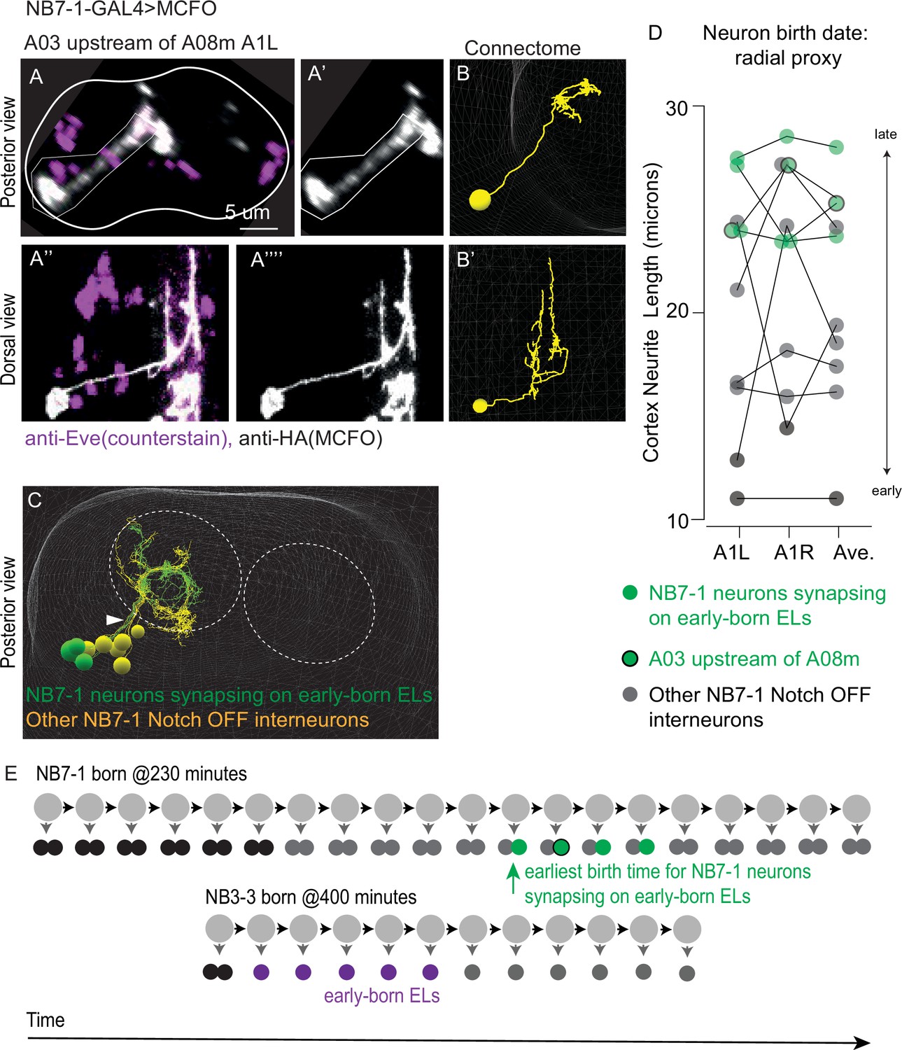
Interneurons from the NB7-1 Notch OFF hemilineage synapse onto early-born ELs and are born after early-born ELs.
(A–C) Images of neuron A03 upstream of A08m, an interneuron from the Notch OFF NB7-1 hemilineage. (A) A confocal image shows a labeled neuron A03 upstream of A08m. This clone was generated using multi-color flip out driven by NB7-1-GAL4. In (A) and (A’’), an anti-Eve counterstain is also shown. Image borders are noted and the outline of the central nervous system (CNS) is shown in (A). The confocal image is shown adjacent to the matching neuron in the connectome (B, B’). (C) An image of all interneurons in the NB7-1 Notch OFF hemilineage in segment A1L is shown. The neuropil is outlined by dashed circles. Neurons that synapse onto early-born ELs are in green, and other neurons in the hemilineage are in yellow. Arrowhead points to the lineage bundle. For genotype, see Supplementary file 4. (D) Quantification of neuron A03 upstream of A08m and other NB7-1 interneurons cortex neurite length. The birth order of A03 interneurons in the NB7-1 Notch OFF hemilineage was estimated using cortex neurite length as a proxy. The Y-axis plots cortex neurite lengths for interneurons in the NB7-1 Notch OFF hemilineage in segment A1L, A1R, and their average. Compared to other neurons in the hemilineage (black), NB7-1 interneurons that synapse onto early-born ELs (green) are born near the end of the lineage. (E) Illustration of NB7-1 and NB3-3 lineage progression showing relative birth timing of early-born ELs and NB7-1 interneurons that synapse onto them. Schematics show a summary of NB7-1 lineage progression compared to NB3-3 lineage progression. Each circle represents one cell with large circles as neuroblasts and smaller circles as neurons. Arrows represent cell division. The X-axis represents developmental time. During the first six divisions, NB7-1 generates motor neurons and undifferentiated siblings (black), and in the remaining divisions generates interneurons (gray and green). NB3-3 starts to divide approximately four divisions than NB7-1. Nonetheless, early-born ELs (magenta) are born before the NB7-1 neurons that synapse onto them (green).
-
Figure 14—source data 1
NB7-1 naming and cortex neurite length.
- https://cdn.elifesciences.org/articles/79276/elife-79276-fig14-data1-v2.xlsx
Additional files
-
Supplementary file 1
Inputs onto NB3-3A1L/R neurons.
With following tabs: All inputs on NB3-3A1L/R neurons (Figure 4A). Left–right paired interneuron inputs (Figure 4D). NB3-3 to NB3-3 connectivity (Figure 11G).
- https://cdn.elifesciences.org/articles/79276/elife-79276-supp1-v2.xlsx
-
Supplementary file 2
Inputs onto early-born ELs.
With following tabs: All sensory neuron and interneuron inputs onto early-born ELs (Figure 6E). Summary (Figure 6EB). Inputs onto early-born ELs (Figure 6B). Input onto each early-born EL (Figure 7B–D).
- https://cdn.elifesciences.org/articles/79276/elife-79276-supp2-v2.xlsx
-
Supplementary file 3
Inputs onto Basins and Ladders.
With following tabs: Basin A1 connectivity (Figures 9F and G and 11G) Basin names (Figure 9). Ladder A1 connectivity (Figures 10F and 11G).
- https://cdn.elifesciences.org/articles/79276/elife-79276-supp3-v2.xlsx
-
Supplementary file 4
Resources.
With the following tabs: Genotypes used in this study. Fly lines antibody list.
- https://cdn.elifesciences.org/articles/79276/elife-79276-supp4-v2.xlsx
-
Supplementary file 5
Names for ELs in A1.
- https://cdn.elifesciences.org/articles/79276/elife-79276-supp5-v2.xlsx
-
Supplementary file 6
Summary of other highly connected interneurons.
- https://cdn.elifesciences.org/articles/79276/elife-79276-supp6-v2.xlsx
-
Transparent reporting form
- https://cdn.elifesciences.org/articles/79276/elife-79276-transrepform1-v2.pdf
Download links
A two-part list of links to download the article, or parts of the article, in various formats.
Downloads (link to download the article as PDF)
Open citations (links to open the citations from this article in various online reference manager services)
Cite this article (links to download the citations from this article in formats compatible with various reference manager tools)
Sequential addition of neuronal stem cell temporal cohorts generates a feed-forward circuit in the Drosophila larval nerve cord
eLife 11:e79276.
https://doi.org/10.7554/eLife.79276


