Modeling and mechanical perturbations reveal how spatially regulated anchorage gives rise to spatially distinct mechanics across the mammalian spindle
- Biophysics Graduate Program, University of California, San Francisco, United States
- Department of Bioengineering and Therapeutic Sciences, University of California, San Francisco, United States
- Biochemistry and Molecular Biophysics Option, California Institute of Technology, United States
- A. Alikhanyan National Laboratory (Yerevan Physics Institute), Armenia
- Division of Biology and Biological Engineering, California Institute of Technology, United States
- Department of Physics, California Institute of Technology, United States
- Chan Zuckerberg Biohub, San Francisco, United States
- Department of Biochemistry and Biophysics, University of California, San Francisco, United States
Figures
Figure 1
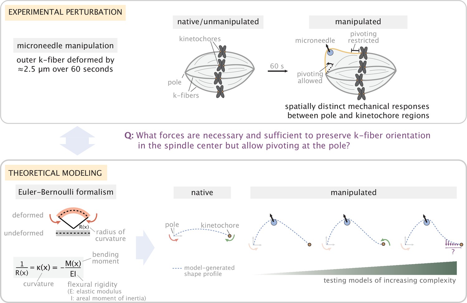
Overview of the experiment-theory interplay used for studying the mechanics of k-fiber anchorage in the mammalian spindle.
Top: Schematic of the experimental perturbation performed in Suresh et al., 2020. Microneedle (blue circle) manipulation of outer k-fibers revealed that k-fibers do not freely pivot near kinetochores, ensuring the maintenance of k-fiber orientation in the spindle center, and pivot more freely around poles. Bottom: Coarse-grained modeling approach of the k-fiber in the spindle context based on Euler-Bernoulli beam theory. Model complexity is progressively increased to identify the minimal set of forces necessary and sufficient to recapitulate (dashed blue lines) k-fiber shapes in the data. From left to right: we test models with different forces and moments at k-fiber ends (pole and kinetochore) to recapitulate native k-fibers, and, then test models of increasing complexity (first with x- and y- force components and just a moment at the pole, then a moment at the kinetochore and finally lateral anchorage over different length scales along the k-fiber (purple arrows)) to recapitulate manipulated k-fibers. Here, forces (represented as straight arrows) and moments (represented as curved arrows) together define the bending moment M(x) along the k-fiber, while k-fiber shape is determined via curvature κ(x).
Figure 2 with 3 supplements
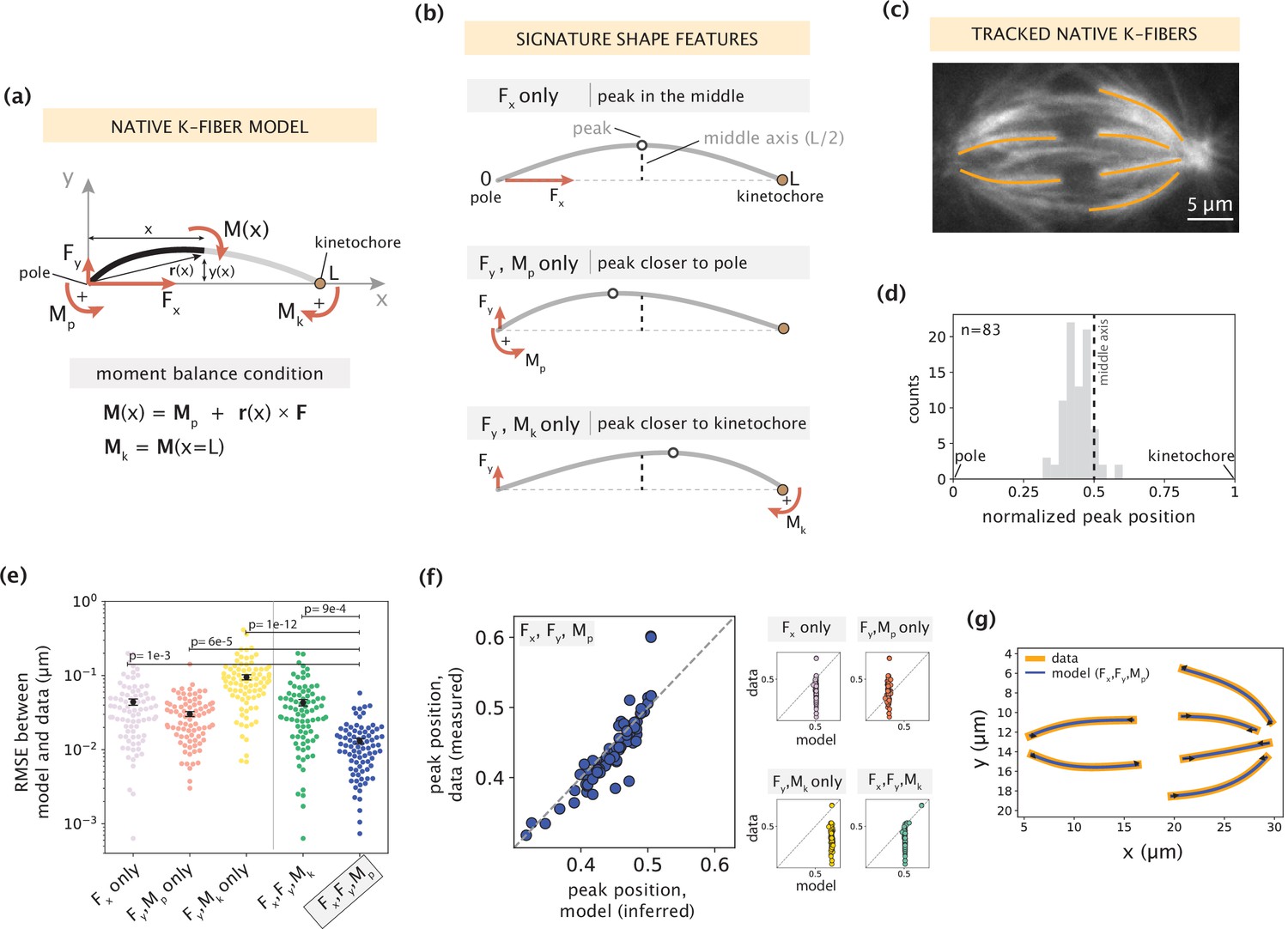
Forces and moments acting on k-fiber ends alone can capture native mammalian k-fiber shapes.
See also Figure 2—figure supplements 1–3. (a) Schematic of the minimal model for native/unmanipulated k-fibers. Pole and kinetochore ends are oriented along the x-axis (x from 0 to L). Only forces (Fx, Fy; red linear arrows) and moments (Mp, Mk; red curved arrows) acting on k-fiber ends are considered. The moment balance condition M(x) shown below defines the k-fiber shape at every position via the Euler-Bernoulli equation. (b) The unique mechanical contribution of each model component to a signature shape feature of native k-fibers. The white circle denotes the k-fiber’s peak position (location where the deflection y(x) is the largest). Each component uniquely shifts the peak position relative to the middle axis (dashed line at x=L/2). (c) Representative image of a PtK2 GFP-tubulin metaphase spindle (GFP-tubulin, white) with tracked k-fiber profiles overlaid (orange). (d) Distribution of peak positions of native k-fibers tracked from PtK2 GFP-tubulin cells at metaphase (m=26 cells, n=83 k-fibers), normalized by the k-fiber’s end-to-end distance, with the middle axis (black dashed line) at x=0.5. (e) Root-mean-squared error (RMSE) between the experimental data (m=26 cells, n=83 k-fibers) and the model-fitted shape profiles. Plot shows mean ± SEM. (f) Comparison of normalized peak positions between the experimental data (m=26 cells, n=83 k-fibers) and model-fitted shape profiles for each model scenario. The model with Fx, Fy and Mp (blue points) best captures the peak positions in the data (Pearson R2 coefficient = 0.85, p=7e-22). Black dashed line corresponds to an exact match of peak positions between the model prediction and measurement data. (g) Tracked k-fiber profiles from the spindle image (c) and their corresponding model fits performed with the minimal model with Fx, Fy and Mp, but not Mk. Black arrows represent the model-inferred forces at end-points.
Figure 2—figure supplement 1
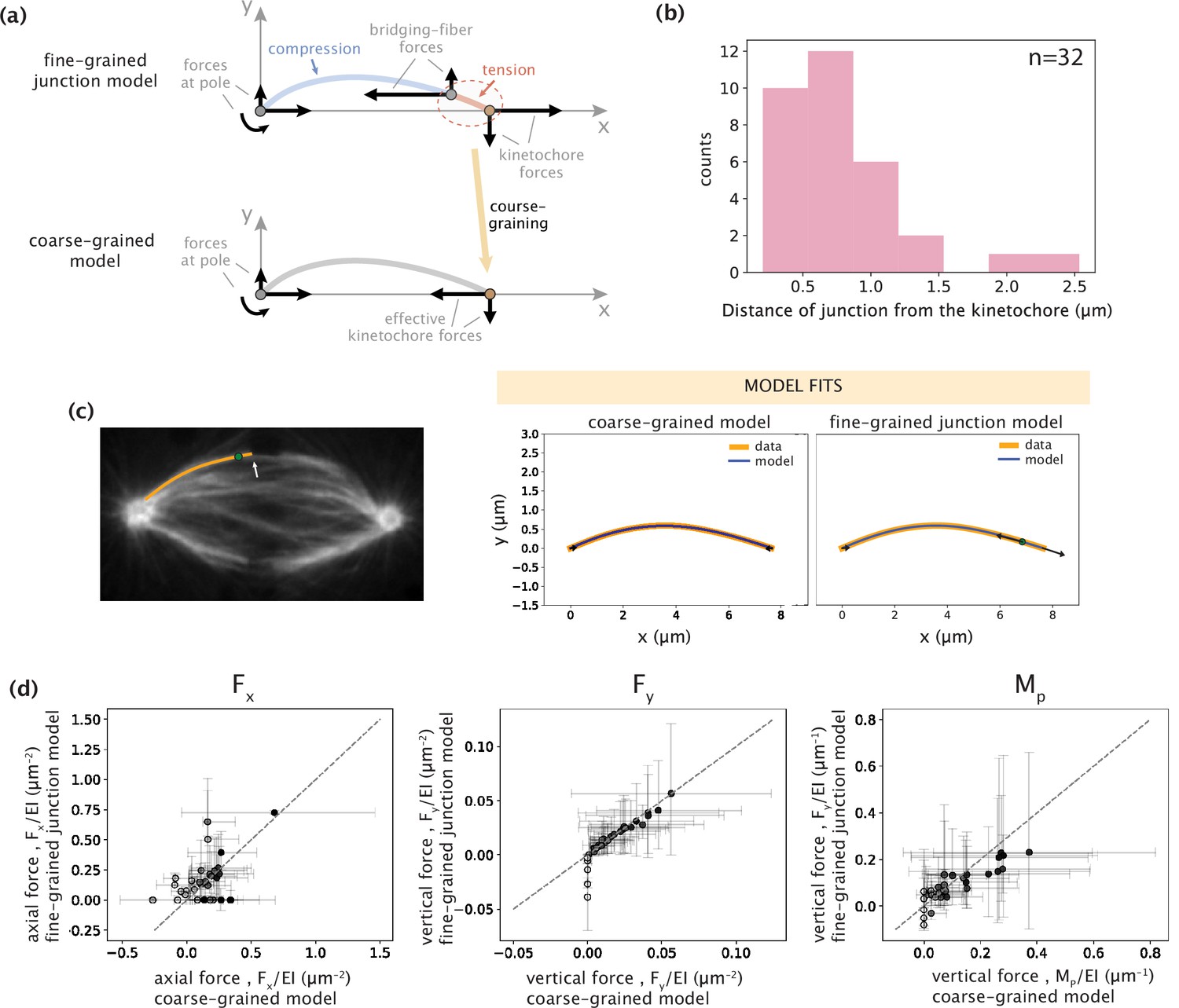
Coarse-graining of kinetochore-proximal tensile and compressive forces to an effective point force at the kinetochore does not alter model outcomes.
(a) Schematic representations of fine- and coarse-grained native k-fiber models. Top: Junction model with a tensile force at the kinetochore and a compressive force near the kinetochore at the bridging-fiber junction. Bottom: Coarse-grained model where the kinetochore-proximal forces are coarse-grained to an effective point force at the kinetochore. (b) Distribution of the distances of the bridging-fiber junction from the kinetochore-end. (c) Left: Representative image of a PtK2 GFP-tubulin metaphase spindle (GFP-tubulin, white) with a tracked k-fiber profile (orange) and bridging-fiber junction (green dot) overlaid. The white arrow points at the bridging-fiber. Right: Tracked k-fiber profile from the spindle image (c,left) and the corresponding model fits performed with the minimal coarse-grained model (Fx, Fy, and Mp) and the junction model. Arrows indicate the inferred forces. (d) Comparison of the three force parameters (left: Fx, middle: Fy, and right: Mp) inferred from the coarse-grained model (x-axis) and the junction model (y-axis). Color of points (light to dark) corresponds to the weight of shape contribution for the three force parameters calculated as: wFx = |Fx|ymax/(|Fx|ymax +Mp), and wRy/Mp = Mp/(|Fx|ymax +Mp). Gray dashed-line corresponds to an exact match between the parameters inferred with the two models.
Figure 2—figure supplement 2
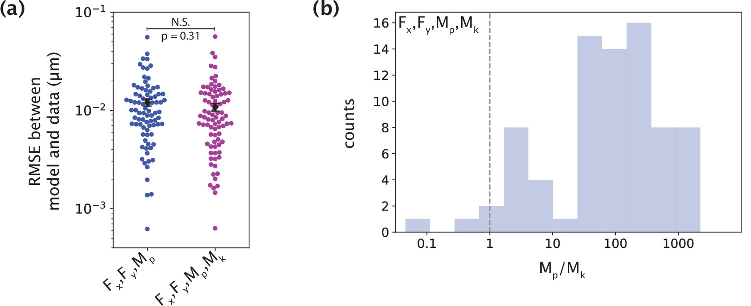
The minimal model does not require a moment at the kinetochore to capture native k-fiber shapes.
(a) Root-mean-squared error (RMSE) between the experimental data (m=26 cells, n=83 k-fibers) and the model fitted shape profiles performed for the model with F (Fx, Fy) and Mp, without (blue) and with (purple) Mk. Plot shows mean ± SEM. (b) Distribution (log scale on the x-axis) of the ratio of the inferred values of Mp and Mk for the model with F, Mp and Mk. The black dashed line is where Mp = Mk. In most cases, Mp is significantly larger than Mk.
Figure 2—figure supplement 3
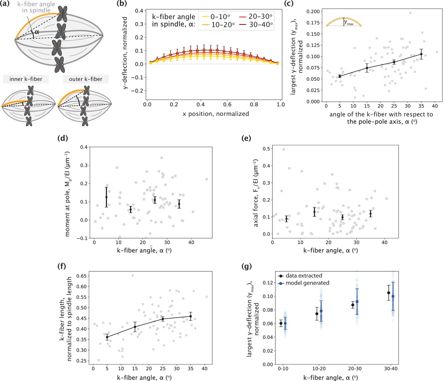
No detectable trend between inner and outer k-fibers is observed in the parameters inferred by the minimal model.
(a) Schematic showing the angle between the k-fiber’s pole-kinetochore axis and the spindle’s pole-pole axis (α). An example of an inner k-fiber having low α and an outer k-fiber having high α is depicted below. (b) Averaged native k-fiber profiles (data) normalized by end-to-end distance (L) and binned according to k-fiber angle in the spindle (α) in 10o increments, with error bars representing the standard deviation of the profiles within the corresponding bin. (c) The largest y-deflection (ymax) for all native k-fiber profiles (data) plotted as a function of their angle in the spindle (α). Outer k-fibers have larger ymax values. Plot shows mean ± SEM. (d-e) Moment at the pole Mp (d) and Fx (e) inferred for the minimal model (F and Mp) fits plotted as a function of the k-fiber angle in the spindle (α) shows no detectable difference across different angles. Plot shows mean ± SEM. (f) K-fiber length, normalized to the spindle’s pole-pole distance (data) plotted as a function of k-fiber angle in the spindle (α) shows increase in length from inner to outer k-fibers. (g) Largest y-deflection (ymax) of k-fiber profiles as a function of their angle in the spindle (α) as calculated from the data in (c) (black) and as captured by the minimal native k-fiber model (blue) only through increasing k-fibers lengths with the angle α (blue). To generate the model profiles, the moment at the pole (Mp) and the axial force (Fx) were taken as their average inferred values and the k-fiber length (Lcontour) was chosen by calculating <Lcontour/dPP> for all k-fibers in each bin (see (f)) and multiplying it by the mean pole-pole distance over all spindles, dPP = 16.27 ± 0.78 μm. Error bars for model estimates were obtained by accounting for the errors (SEM) in estimating Mp, Fx, <Lcontour/dPP>, and dPP.
Figure 3 with 3 supplements

Manipulated k-fiber response cannot be captured solely by end-point anchoring forces and moments.
See also Figure 3—figure supplements 1–2 and Figure 3—video 1. (a) Top: Representative images of a PtK2 spindle (GFP-tubulin, white) before and at the end of microneedle manipulation. Tracked k-fiber profiles (orange) and the microneedle (white circle) are overlaid (shifted for k-fiber) on the images. Bottom: Curvature profiles along the native/unmanipulated and manipulated k-fibers. Time in min:sec. Scale bar = 5 μm. (b) Schematic of the model for the manipulated k-fiber that includes F (Fx, Fy), Mp and Mk is set to zero (minimal native k-fiber model), along with an external force Fext from the microneedle (blue circle). The moment balance condition is shown below, where the indicator function (I) specifies the region over which the corresponding term in the equation contributes to M(x). (c) Top: Manipulated shape profile extracted from the image in (a) (orange line), together with the best fit profile generated by the model (blue line) where Mk = 0. Stars denote the minimum of the negative curvature. The model does not capture the negative curvature observed in the data (orange star). Bottom: Curvature profiles along the k-fiber in the data (left) and the model (right). (d) Schematic of the model for the manipulated k-fiber defined by the parameters in (b) and a negative moment at the kinetochore, Mk (orange arrow). (e) Top: Manipulated shape profile extracted from the image in (a) (orange line), together with the best fit profile generated by the model (blue line) with Mk≠0. Stars denote the minimum of the negative curvature. The model generates a negative curvature (blue star) but cannot accurately capture its position from the data (orange star). Bottom: Curvature along the k-fiber in the data (left) and the model (right). (f) Root-mean-squared error (RMSE) between the experimental data (m=18 cells, n=19 k-fibers) and the best fitted profiles from the models without (Mk = 0) and with (Mk≠0) a moment at the kinetochore. A comparison is made also with the RMSE of the minimal native k-fiber model (control, Figure 2a). Plots show mean ± SEM. (g–i) Comparison of manipulated k-fiber profiles (m=18 cells, n=19 k-fibers) between the data and model (Mk≠0) for (g) positions curvature maxima (Pearson R2 coefficient = 0.95, p=4e-13), (h) positions of curvature minima (Pearson R2 coefficient = 0.27, p=1e-1), and (i) the distance over which the orientation angle is preserved within 1o (Pearson R2 coefficient = 0.43, p=9e-4).
Figure 3—figure supplement 1
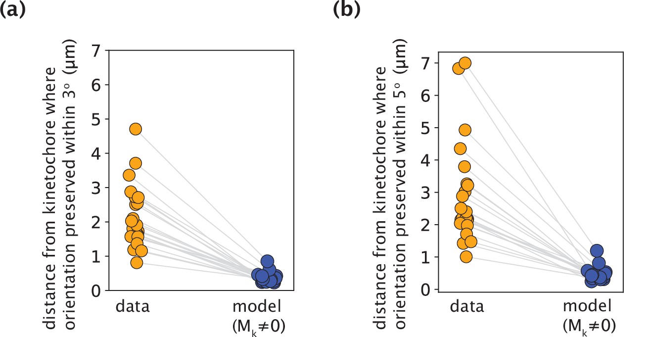
K-fiber orientation in model profiles with Mk≠0 is preserved over much shorter distances than in experimental data, irrespective of the chosen threshold angle.
(a,b) The distance from the kinetochore where the orientation angle is preserved within 3o (a) and 5o (b), calculated for all measured experimental data and model-fitted profiles (m=18 cells, n=19 k-fibers). Grey lines link the corresponding profiles.
Figure 3—figure supplement 2
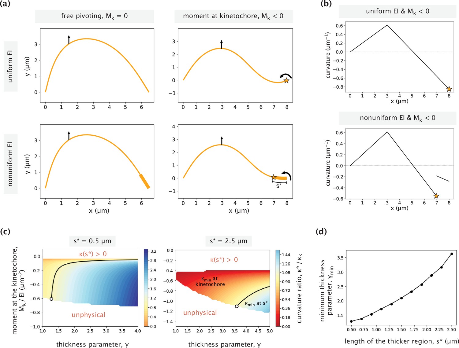
Impact of nonuniform flexural rigidity on the k-fiber response to force.
(a) Example k-fiber responses to external manipulation in the presence/absence of a point bending moment Mk at the kinetochore for cases with a uniform (top panels) and nonuniform (bottom panels) flexural rigidity. Parameters used: Mk = –0.85 EI μm–2 (for the two panels on the right), s*=1 μm and γ=3 (for the two panels on the bottom). A vertical force is applied 5 μm horizontal distance away from the kinetochore in all cases. The stars indicate positions of negative curvature minima. (b) Curvature variations as a function of x-position for the cases with a uniform (top) and nonuniform (bottom) flexural rigidities. The same point moment at the kinetochore is applied in both cases. (c) Ratio of the negative curvature at s* and the negative curvature at the kinetochore for different choices of the thickness parameter (γ) and the moment at the kinetochore (Mk). Two different cases of s* are considered (s*=0.5 µm, 2.5 µm). The curvature ratio is equal to 1 along the black contour line. To the right of the line, the curvature minimum is at s* and to the left of it, the minimum is at the kinetochore. Regions of the parameter space where either the curvature at s* was positive (top part) or the k-fiber has an unphysical profile (bottom part), are left blank and labeled in red. The white circle in each case indicates the parameter combination at the transition contour with the lowest value of γ. (d) Minimum thickness parameter (γ) necessary for having the curvature minimum away from the kinetochore, calculated for different contour lengths of the higher flexural rigidity region (s*). White circles on the two heatmaps (c) correspond to the points on the plot with s*=0.5 μm and s*=2.5 μm.
Figure 3—video 1
Microneedle manipulation of PtK2 metaphase spindles reveals the restriction of k-fiber pivoting around the kinetochore but not the pole.
Microneedle manipulation of a metaphase spindle in a PtK2 (GFP-tubulin, white) cell. The microneedle (Alexa-647, white circle) exerts a force on the outer k-fiber over 60 s to mechanically challenge its anchorage to the spindle. The k-fiber is restricted from freely pivoting near the chromosome (negative curvature, orange arrow) and maintains a straight orientation, but is able to pivot at the pole, thereby giving rise to spatially distinct mechanical responses across the different regions of the spindle. Time in min:sec. Video was collected using a spinning disk confocal microscope, at a rate of 1 frame every 7 s before and during manipulation. Video has been set to play back at constant rate of 5 frames per second. Movie corresponds to still images from Figure 3a.
Figure 4 with 4 supplements
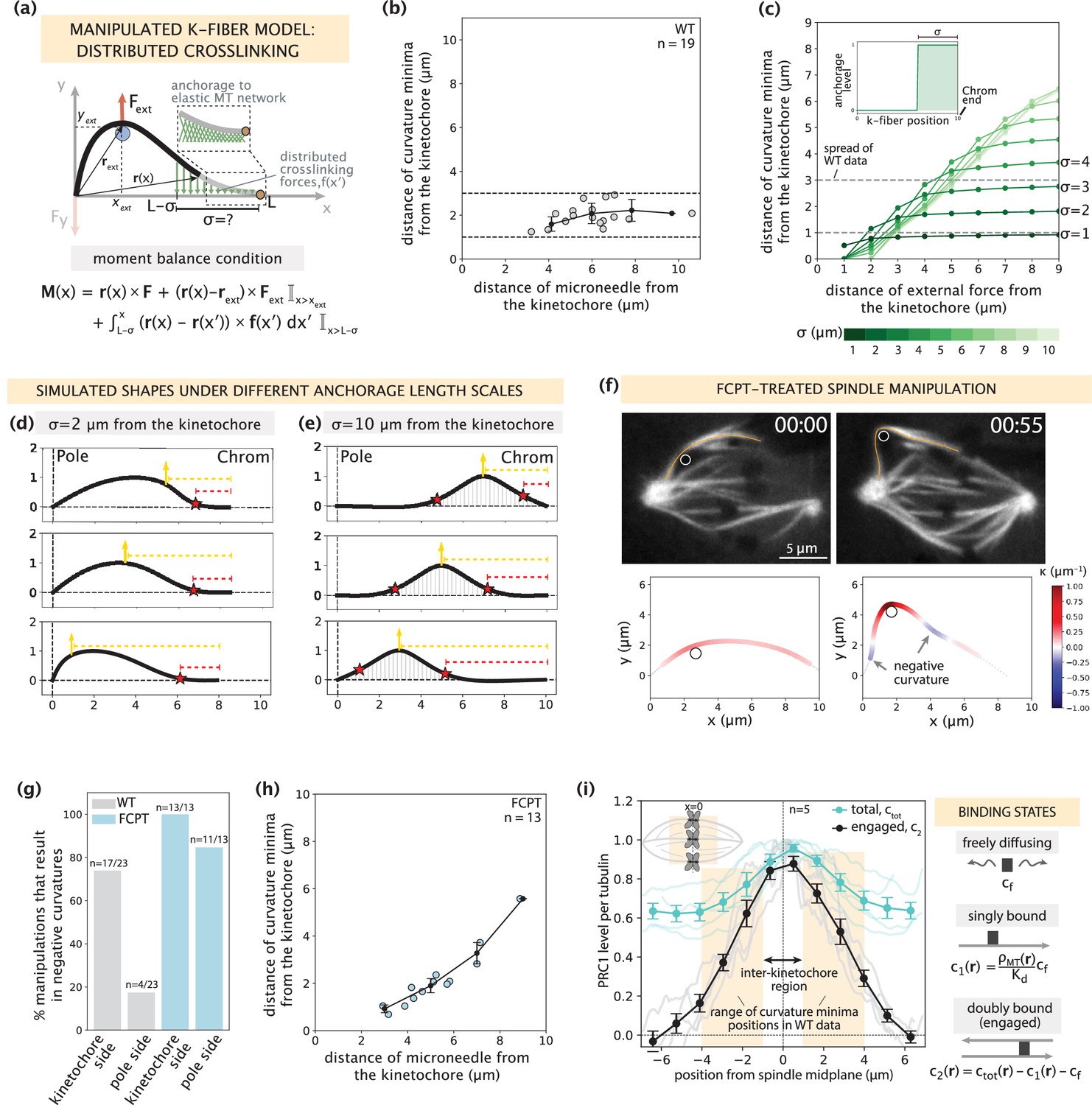
Mapping the relationship between anchorage length scales and manipulated k-fiber shapes constrains the spatial distribution of lateral anchorage.
See also Figure 4—figure supplements 1–3 and Figure 4—video 1. (a) Schematic of the model for the manipulated k-fiber with crosslinking forces f(x′) distributed over a length scale σ near the kinetochore. The model also includes endpoint forces F, and an external force from the microneedle Fext. The crosslinking force density is f(x′) = -k y(x′) ŷ, where k is the effective spring constant and ŷ is the unit vector in the y direction. Since we do not expect Mp to influence the crosslinking behavior near the kinetochore, for simplicity we set Mp = 0 in simulation studies of this section. Indicator function (I) in the moment balance condition specifies the region over which the corresponding term contributes to M(x). (b) Distance of curvature minima as a function of distance of the microneedle from the kinetochore (m=18 cells, n=19 k-fibers), in wildtype spindle manipulations (Suresh et al., 2020). Plot shows mean ± SEM (black). (c) Distance of curvature minima as a function of distance of external force application from the kinetochore calculated for model-simulated profiles where the length scale of anchorage (σ, inset) is tuned in the range 1–10 μm (denoted by shades of green). Variation of the position of external force application mimics the wildtype manipulation experiments in (b). Dashed lines denote the spread of curvature minima positions in (b). (d,e) Profiles generated by the model in (a) with (d) σ=2 μm and (e) σ=10 μm for varying positions of external force application (yellow arrow), and the resulting positions of curvature minima (red star). Dashed lines represent the distances from the kinetochore to the external force position (yellow dashed line) and curvature minimum position (red dashed line). (f) Top: Representative images of a PtK2 spindle (GFP-tubulin, white) treated with FCPT to rigor-bind the motor Eg5, in its unmanipulated (00:00) and manipulated (00:55) states. The microneedle (white circle) and tracked k-fibers (orange) are displayed on images. Bottom: Curvature along the tracked k-fibers. Time in min:sec. (g) Percentage of microneedle manipulations that gave rise to a negative curvature near the kinetochore and the pole in wildtype (grey; m=18 cells, n=19 k-fibers, Suresh et al., 2020) and FCPT-treated (light blue; m=11 cells, n=13 k-fibers) spindles. (h) Distance of curvature minima as a function of distance of the microneedle from the kinetochore in FCPT-treated spindle manipulations (m=9 cells, n=13 k-fibers). Plot shows mean ± SEM (black). (i) Left: Normalized distribution of PRC1’s total abundance levels (ctot, cyan lines) measured from immunofluorescence images (fluorescence intensity, n=5 cells) (Suresh et al., 2020) and actively engaged (doubly bound, c2, grey lines) PRC1 calculated from the ctot using the equilibrium binding model along the spindle’s pole-pole axis (x=0 represents the spindle midplane). The region along k-fibers where negative curvature is observed in the wildtype dataset is highlighted in orange and the inter-kinetochore region (double-sided black arrow) denotes the chromosome region between the sister k-fibers (inset). Plot shows mean ± SEM for both PRC1 populations. Right: Three distinct binding states of PRC1 considered in our analysis. The concentration of actively engaged PRC1 (c2) is calculated by subtracting the free and singly bound contributions from the total PRC1 concentration (ctot). In the expression for the singly-bound PRC1 population, ρMT(r) stands for the local tubulin concentration, while Kd represents the dissociation constant of PRC1– single microtubule binding.
Figure 4—figure supplement 1
Tuning anchorage strength within an order of magnitude only introduced sub-micron variations in the negative curvature response.
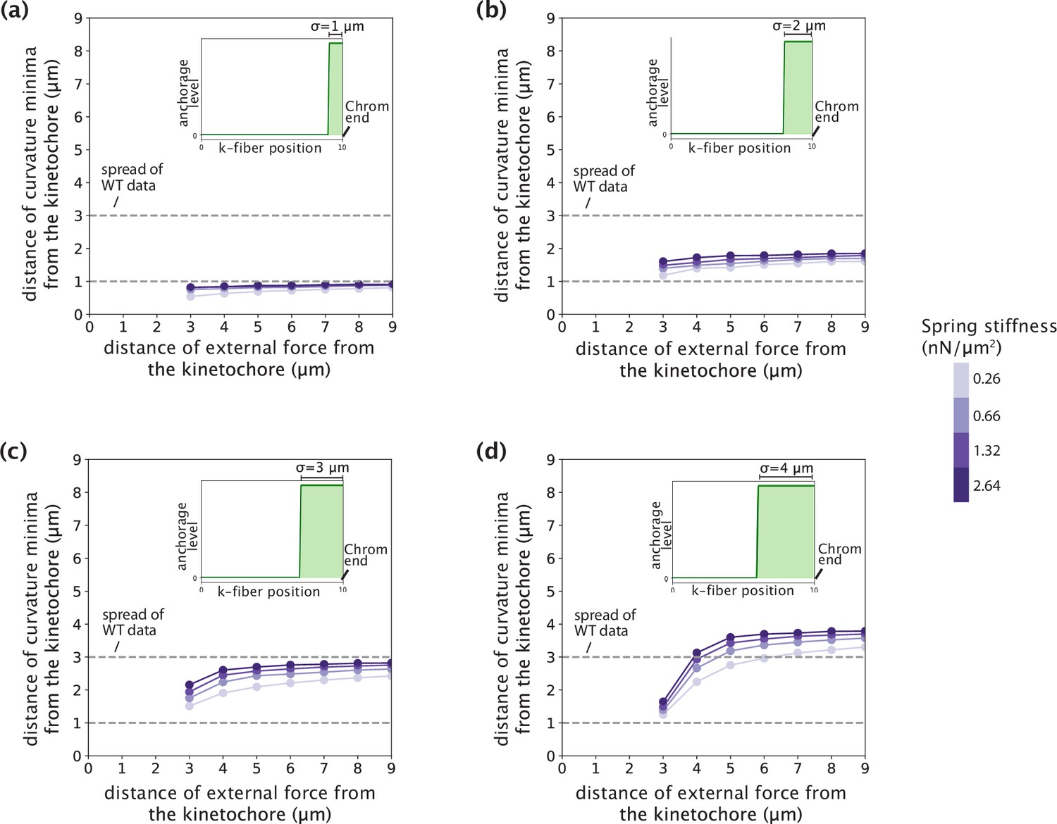
(a–d) Distance of curvature minima from the kinetochore as a function of the position of external force application. Distances are calculated for model-simulated profiles where the anchorage strength (spring stiffness k that enters the crosslinking force density via f(x′) = -k y(x′) ŷ) is tuned from 0.2 to 2 nN/μm2 (an order of magnitude) for different anchorage length scales (σ=1 μm (a), σ=2 μm (b), σ=3 μm (c), σ=4 μm (d)). Dashed lines denote the spread of curvature minima positions in Figure 4b.
Figure 4—figure supplement 2

Microneedle displacement over time in FCPT-treated spindle manipulations.
Blue lines represent individual manipulations. Plot shows mean ± SD (black).
Figure 4—figure supplement 3

Negative curvature does not remain localized near chromosomes when anchorage levels in the model mimic PRC1 intensity in the spindle.
(a) Distribution of PRC1 abundance normalized to tubulin (fluorescence intensity, n=5 cells) along the spindle’s pole-pole axis from the midplane (x=0 where chromosomes are, left inset) to each pole, measured from immunofluorescence images of spindles (right inset, white box denotes the region over which intensity was measured) (Suresh et al., 2020). Plot shows mean ± SEM. (b,c) Distance of curvature minima as a function of distance of external force application from the kinetochore in an anchorage scenario mimicking normalized PRC1 abundance (a) with an enrichment of up to 3 μm near the kinetochores and a 60% basal level along the k-fiber as a (b) step function and (c) gaussian distribution. Anchorage levels in space for each scenario are shown in insets.
Figure 4—video 1
Microneedle manipulation of FCPT-treated PtK2 spindles reveals negative curvature on both sides of the microneedle and not localized near kinetochores.
Microneedle manipulation of a metaphase spindle in a PtK2 (GFP-tubulin, white) cell treated with FCPT to rigor-bind the motor Eg5. The microneedle (Alexa-647, white circle) exerts a force on the outer k-fiber over 60 s to mechanically challenge its anchorage to the spindle. The k-fiber is restricted from freely pivoting near the chromosome (negative curvature, orange arrowhead) and near the pole (negative curvature, yellow arrow), leading to a loss of mechanical distinction between the two regions. The negative curvature also does not remain localized near the chromosome (unlike in control spindles), and is instead away from the chromosome (orange line) and closer to the microneedle. Time in min:sec. Video was collected using a spinning disk confocal microscope, at a rate of 1 frame every 8 s before and during manipulation. Video has been set to play back at constant rate of 5 frames per second. Movie corresponds to still images from Figure 4f.
Figure 5 with 2 supplements
Minimal k-fiber model infers strong lateral anchorage within 3 μm of kinetochores to be necessary and sufficient to recapitulate manipulated shape profiles.
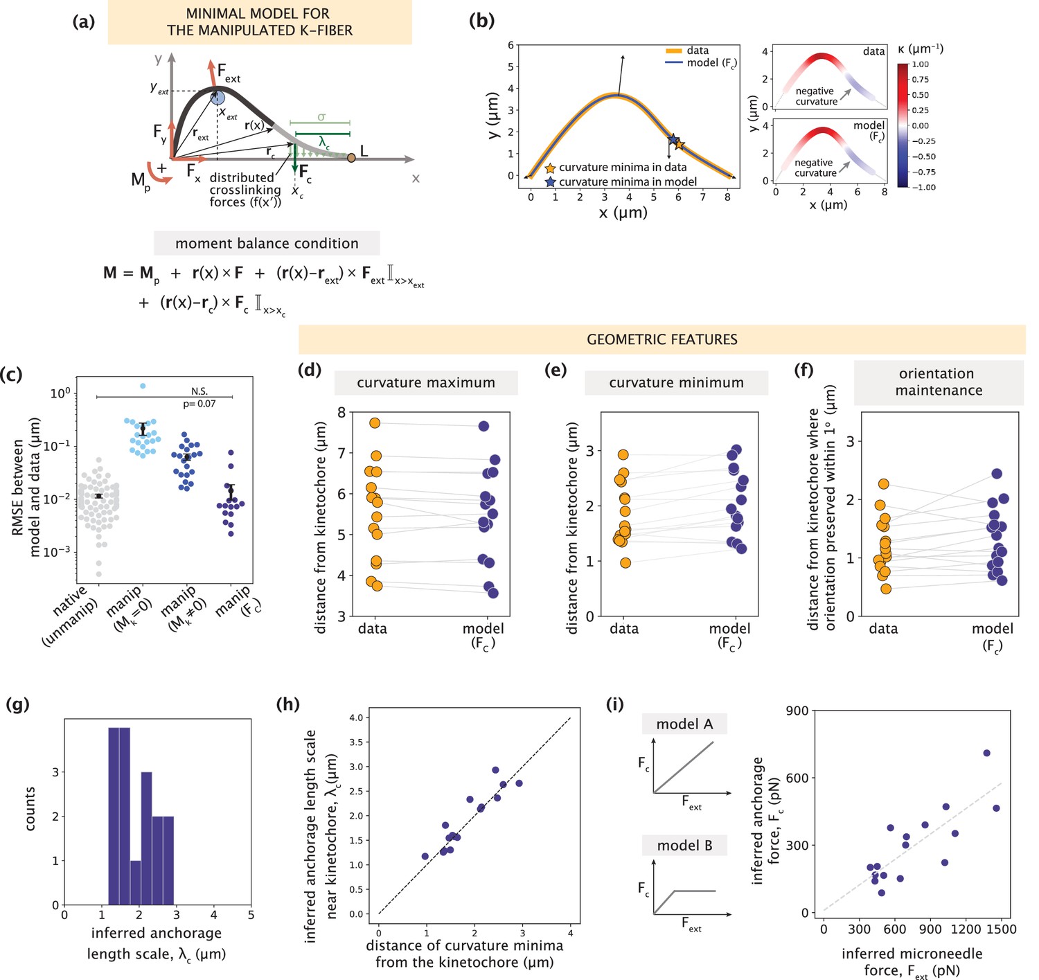
See also Figure 5—figure supplements 1–2. (a) Schematic of the model for the manipulated k-fiber with an effective point crosslinking force (Fc, dark green arrow) a distance λc away from the kinetochore-end introduced to capture the effect of the distributed crosslinking forces (light green arrows) localized near the kinetochore. The model also includes the parameters F, Mp and Fext. Indicator function (I) in the moment balance condition specifies the region over which the corresponding term contributes to M(x). (b) Left: Manipulated shape profile extracted from the image in Figure 3a (orange line), overlaid with the best fitted profile inferred by the model with Fc (blue line). Black arrows represent the model-inferred forces that correspond to (a). Stars denote the minimum of the negative curvature, which matches well between the data (orange star) and model (blue star). Right: Curvature along the k-fiber in the data (top) and the model (bottom). (c) Root-mean-square error (RMSE) between the experimental data and all k-fiber models tested: Mk = 0 (Figure 3b), Mk≠0 (Figure 3d) and Fc (Figure 5a). A comparison is made with the minimal native k-fiber model (control, Figure 2a). Plot shows mean ± SEM. (d-f) Comparison of manipulated k-fiber profiles (m=14 cells, n=15 k-fibers) between the data and model (Fc) for (d) positions curvature maxima (Pearson R2 coefficient = 0.97, p=8e-12), (e) positions of curvature minima (Pearson R2 coefficient = 0.9, p=1e-7), and (f) the distance over which the orientation angle is preserved within 1o (Pearson R2 coefficient = 0.85, p=2e-4). Grey lines link the corresponding profiles. (g) Distribution of the length scales of anchorage (λc) inferred by the minimal model with Fc for all k-fibers in the data. (h) Positions of curvature minima extracted from data profiles vs. the location of the effective crosslinking force near kinetochores inferred by the model (Pearson R2 coefficient = 0.85, p=1e-6), with the black dashed line representing perfect correspondence between them. (i) Left: Possible scenarios for models of how anchorage force Fc might correlate with the microneedle force Fext – linearly as is characteristic to an elastic response (model A), or linearly up to a force threshold, beyond which detachment of anchorage occurs (model B). Right: Microneedle force Fext vs. anchorage force Fc inferred from the model shows a monotonic relationship. Grey dashed line represents the best-fit line (Spearman R coefficient = 0.85, p=4e-4).
Figure 5—figure supplement 1
Validating the use of a point crosslinking force to capture distributed anchorage.
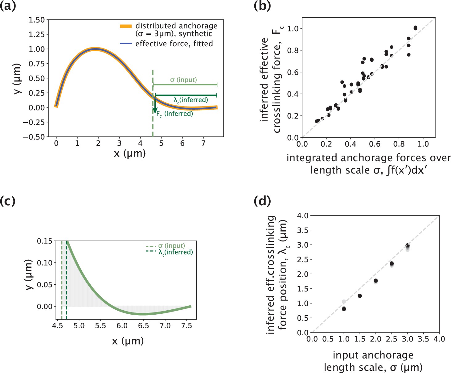
(a) An example simulated k-fiber profile generated by the distributed crosslinking model with σ=3 μm (Figure 4a, orange), and a profile fitted by the model with Fc (Figure 5a, blue) overlaid. (b) Integrated anchorage forces from the simulated profiles plotted against the inferred crosslinking force (Fc), for a range of external force positions (4–8 μm from the kinetochore, denoted by shades of green). The grey dashed line is where Fc = ∫f(x′)dx′. Forces reported are normalized by the flexural rigidity EI, with the units on the axes given by μm–2. (c) Simulated profile from (a) zoomed-in to the anchorage region (3 μm near chromosomes). The y-axis corresponds to anchorage deformation, which is only large near the edge of the anchored region, where Fc is inferred. (d) Input distributed anchorage length scale (σ) that generated the simulated profiles plotted against the inferred effective crosslinking force position (λc), for a range of external force positions (4–8 μm from the kinetochore, denoted by shades of grey). The grey dashed line is where λc = σ.
Figure 5—figure supplement 2
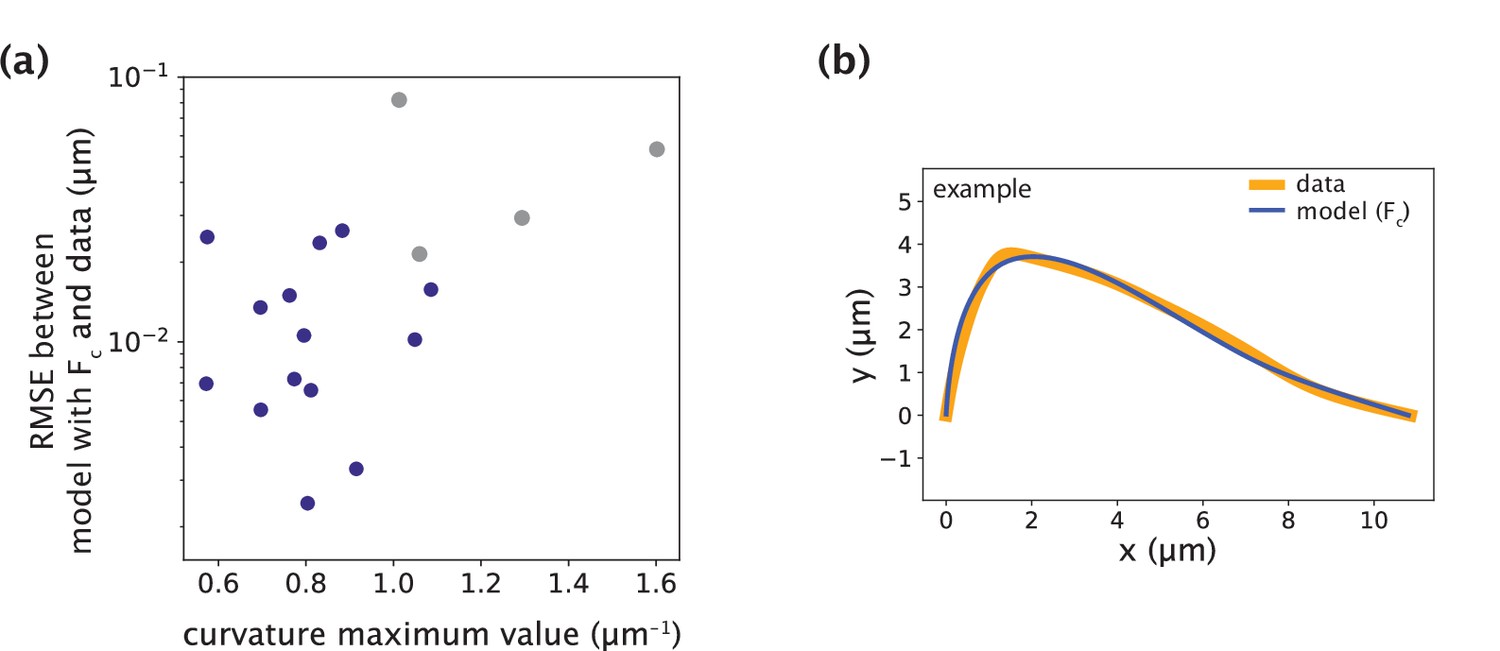
Minimal model with point crosslinking force fails to recapitulate the data only in cases with large positive curvature values.
(a) Root-mean-square error (RMSE) between the data and the minimal model with Fc (Figure 5a) as a function of the maximum curvature value along k-fibers found at the site of microneedle force application. The blue points represent the successful fits with low RMSE and grey points represent the cases where the model fails to fit the data and produces higher RMSE. (b) Example of manipulated shape profile with high positive curvature regions at the site of force application (data, orange) where the model (blue) fails to accurately recapitulate them.
Figure 6
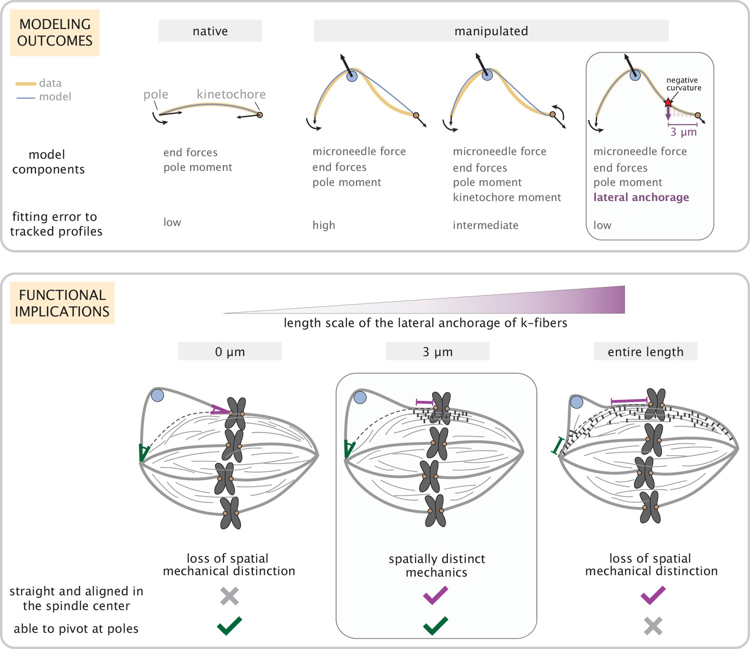
Coarse-grained modeling of k-fiber shapes reveals how spatially regulated k-fiber anchorage gives rise to spatially distinct mechanics across the mammalian spindle.
Top: A summary of outcomes for the native k-fiber model and the various iterations of the manipulated k-fiber model, where we systematically built up model complexity (left to right) to capture the observed shapes. The minimal model (rightmost panel), which produced the best fits, includes forces at k-fiber ends, a moment at the pole, and localized crosslinking forces (captured through an effective point crosslinking force). The minimal model (rightmost panel) also revealed a quantitative and predictive link between the position of the negative curvature (red star) and the length scale of k-fiber anchorage (position of purple arrow from the kinetochore-end). Bottom: Functional implications of models with different length scales of anchorage (0, 3, 10 μm from left to right) tested in our study. Unlike the scenarios with no anchorage and anchorage along the entire length (left and right panel), anchorage up to 3 μm from the kinetochore (middle panel) is best suited to ensure that k-fibers remain straight in the spindle center and aligned with their sister (purple line), while also allowing them to pivot and focus at the pole (green pivot point).
Appendix 1—figure 1
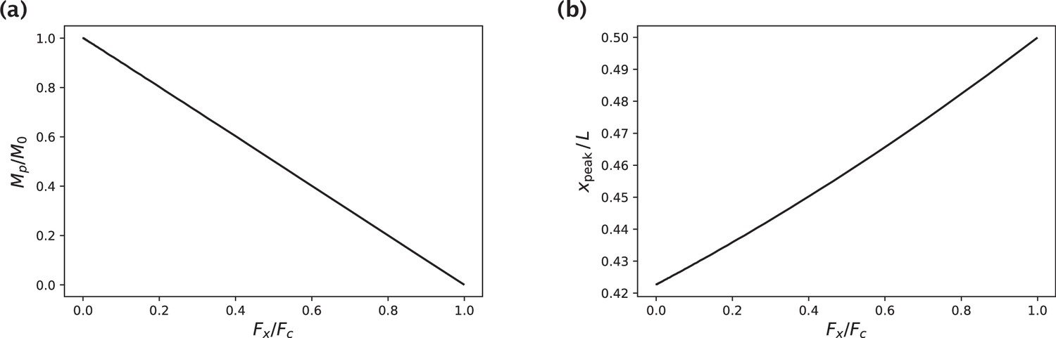
Generation of native k-fiber shapes with a fixed peak deflection ymax for different choices of the axial force .
(a) Moment at the pole that yields the specified peak deflection ymax as a function of . M0 is the pole moment in the absence of an axial force. (b) -position of the profile peak as a function of.
Appendix 1—figure 2
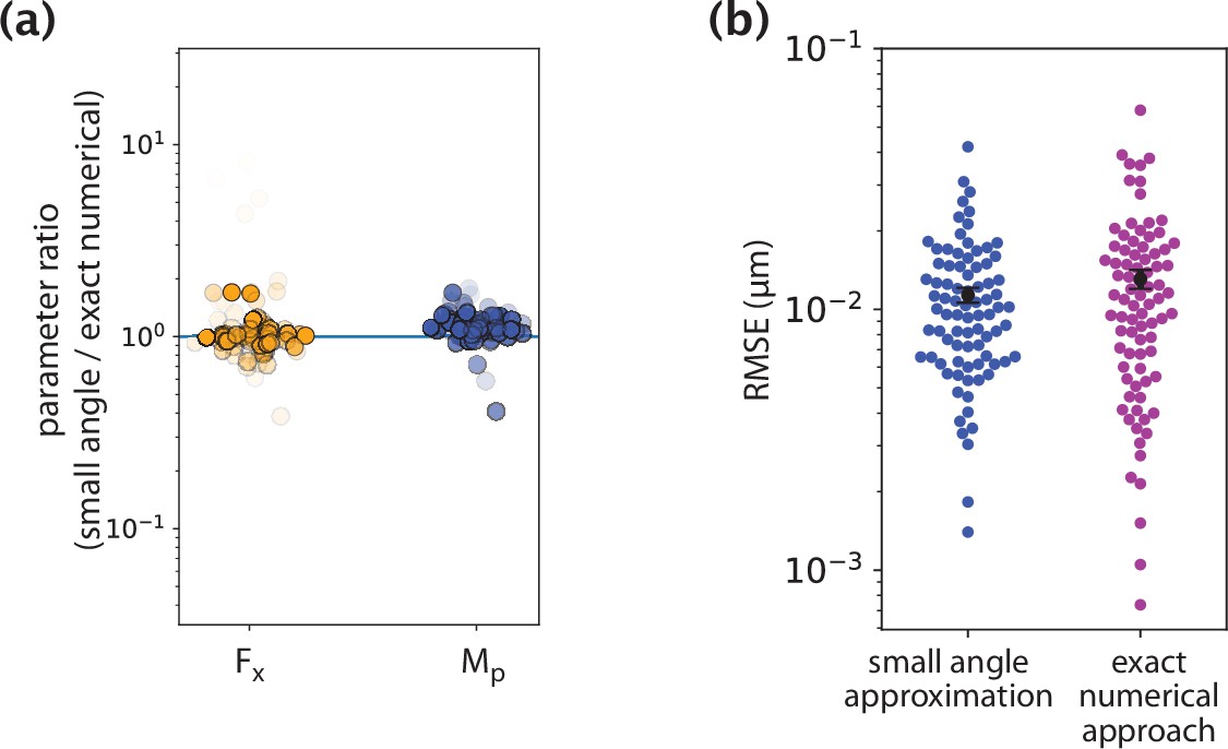
Comparison of inference results from the small angle approximation and exact numerical approach.
(a) Ratios of parameters inferred by the two methods. (b) Fitting error comparison between the two methods.
Appendix 1—figure 3
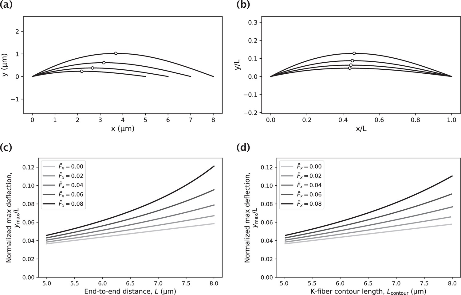
Impact of the k-fiber length on the amount of k-fiber deflection.
(a) Set of k-fiber profiles of varying contour length generated by a moment at the pole and an axial force . Circles indicate the locations of the highest deflection. (b) K-fiber profiles in panel (a), normalized by the end-to-end distance . (c) Dependence of the normalized maximum deflection on the end-to-end distance for varying choices of the axial force (reported in units of ) and a fixed value of the moment at the pole, . (d) Study in panel (c) with the -axis corresponding to the k-fiber contour length instead of the end-to-end distance .
Appendix 2—figure 1
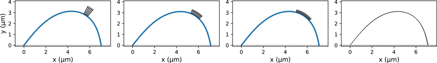
K-fiber profile generation with a distributed microneedle force.
(a) Example profiles where the same integrated microneedle force was applied over three different regions of the k-fiber. The black arrows indicate the applied external forces with lower magnitudes for larger regions of distributed force application. Parameters used in profile generation: (integrated force), µm. (b) Profiles from 10 different distributed force settings overlaid on top of each other. Only minor differences can be observed near the rightmost end.
Appendix 2—figure 2
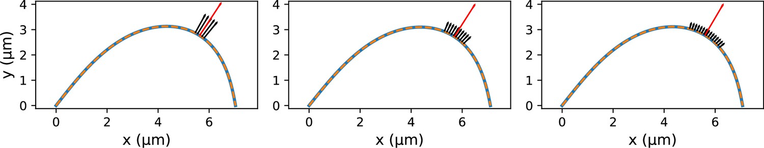
Fits of the point microneedle force model (dashed lines) to synthetic profiles (solid blue lines) which were generated with distributed forces applied over different regions.
The red arrow indicates the inferred point microneedle force .
Appendix 4—figure 1

Schematic of the error definition.
For the data point, the error di is the smallest distance to the model profile which is represented as a piecewise linear curve. Sum of squared errors, namely, , is minimized in the model fitting procedure.
Appendix 5—figure 1
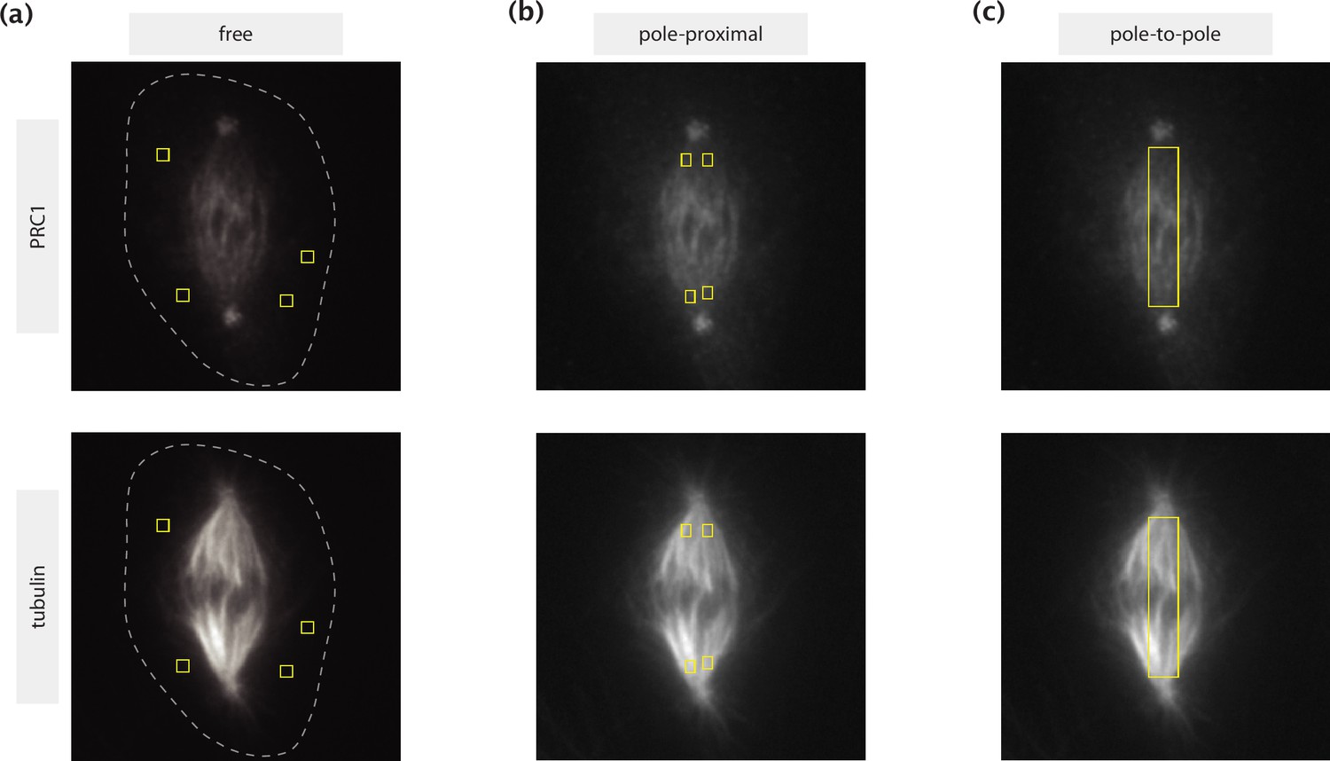
ROIs selected for different calculations shown on immunofluorescence images of PRC1 (top row) and tubulin (bottom row).
(a) Regions with little to no tubulin presence where PRC1 can be considered unbound. The dashed lines represent the cell boundaries estimated by manual tracing based on high intensity contrast. (b) Pole-proximal regions where microtubules are present primarily in a parallel configuration. (c) Rectangular pole-to-pole region where the estimation of the actively engaged PRC1 population is made.
Additional files
Download links
A two-part list of links to download the article, or parts of the article, in various formats.
Downloads (link to download the article as PDF)
Open citations (links to open the citations from this article in various online reference manager services)
Cite this article (links to download the citations from this article in formats compatible with various reference manager tools)
Modeling and mechanical perturbations reveal how spatially regulated anchorage gives rise to spatially distinct mechanics across the mammalian spindle
eLife 11:e79558.
https://doi.org/10.7554/eLife.79558


