Integrative dynamic structural biology unveils conformers essential for the oligomerization of a large GTPase
- Chair for Molecular Physical Chemistry, Heinrich Heine University Düsseldorf, Germany
- Physical Chemistry I, Ruhr University Bochum, Germany
- Jülich Centre for Neutron Science (JCNS-1) and Institute of Biological Information Processing (IBI-8), Forschungszentrum Jülich GmbH, Germany
- Institut für Pharmazeutische und Medizinische Chemie, Heinrich Heine University Düsseldorf, Germany
- Institute of Physical Chemistry, RWTH Aachen University, Germany
- Institut Laue-Langevin, France
- Institute of Bio-Geosciences (IBG-4: Bioinformatics), Forschungszentrum Jülich, Germany
- Macromolecular Structure Group, Department of Physics, University of Osnabrück, Germany
Figures
Figure 1 with 1 supplement
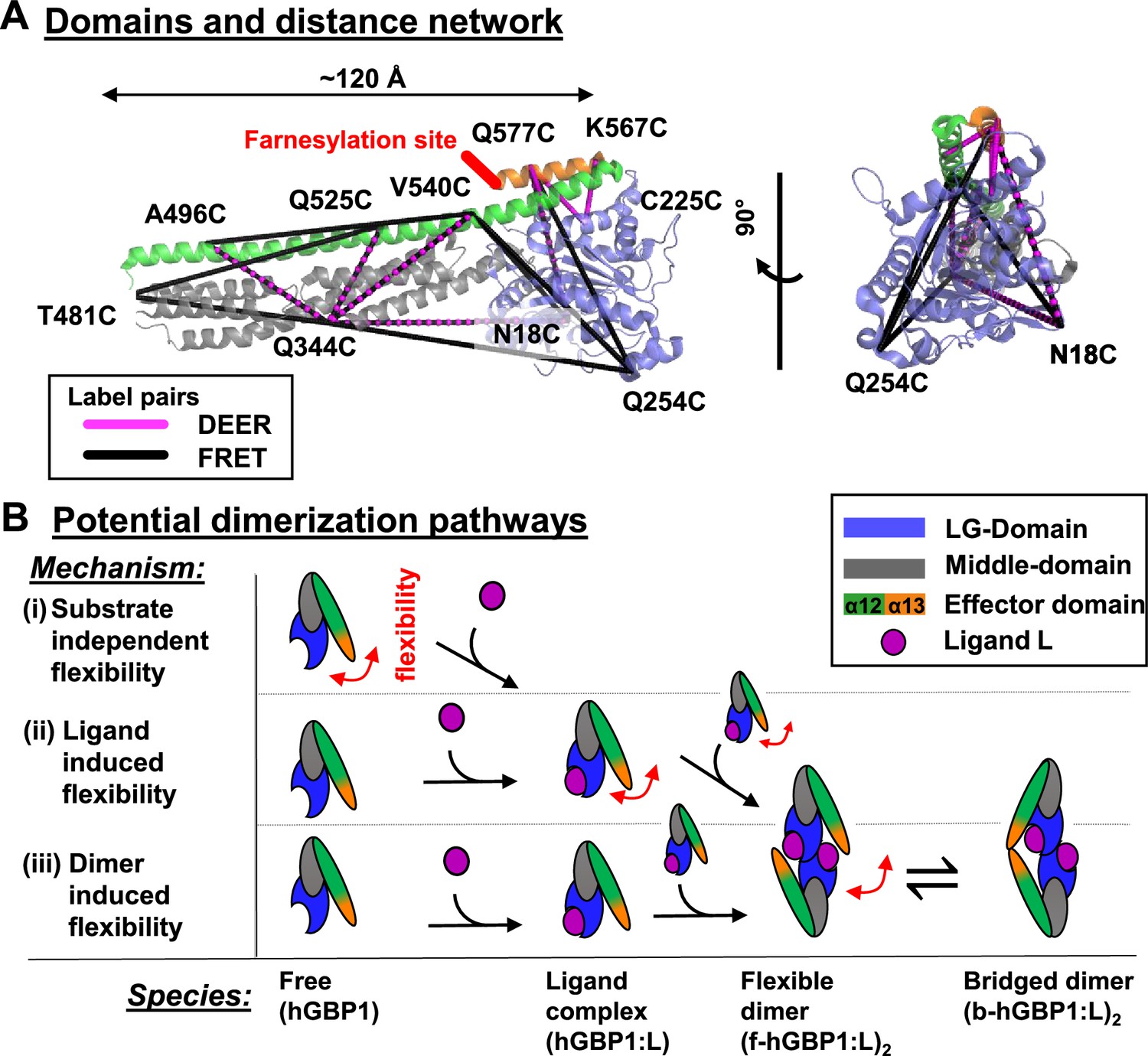
DEER and FRET distance network that probes structural arrangement of the human guanylate binding protein 1 (hGBP1) and potential dimerization pathways.
(A) The network is shown on top of the crystal structure (hGBP1, PDB-ID: 1DG3). hGBP1 consists of three domains: the LG domain (blue), a middle domain (gray) and the helices α12/13 (green/orange). The amino acids highlighted by the labels were used to attach spin-labels and fluorophores for DEER-EPR and FRET experiments, respectively. Magenta and black lines represent the DEER- and FRET-pairs, respectively. In hGBP1 the C-terminus is post-translationally modified and farnesylated for insertion into membranes (red). (B) Potential different pathways for the formation of a functional hGBP1 homodimer where the substrate binding LG domains and the helix α13 associate. The association of the helix α13 requires flexibility (red arrows). This flexibility could be induced at different stages of a dimerization pathway.
Figure 1—figure supplement 1
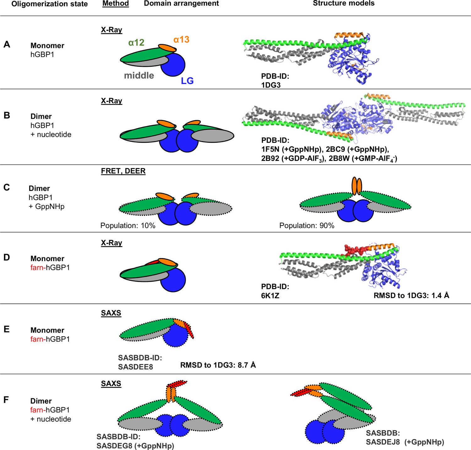
Structural knowledge on hGBP1.
Crystallographic and model-free structural knowledge on hGBP1 is highlighted by solid contour lines of the domains. Model-based and indirect structural information is highlighted by dashed contour lines of the domains. (A) In the crystallographic monomer (PDB-ID: 1DG3) the LG- (blue), middle- (gray), helix α12 (green), and helix α13 (orange) of hGBP1 adopt an extended conformation where helix α12/13 attach to one side of the LG-domain (Prakash et al., 2000). (B) In crystallographic dimer data of the LG-domain (2BC9, 2B92, 2B8W) and in a crystallographic dimer of the full-length protein (PDB-ID: 1F5N) require helix α13 to be located at diastral sites of the LG:LG domain dimer (C) FRET and DEER experiments on hGBP1 verified crystallographic LG:LG domain interaction (solid lines) and identified two dimer conformations. In the minor (10% population) conformation helix α13 were separated. In the major conformation (90% population) two α13 helices associate (Vöpel et al., 2014). (D) A crystallographic structure on farnesylated hGBP1. The farnesyl anchor (red) attached to helix α13 extends along helix α12 and binds between α12 and α13. The farnesylated hGBP1 and the non-farnesylated hGBP1 crystal structures are largely consistent (RMSD 1.4 Å). (E) SEC-SAXS experiments on farnesylated hGBP1 identified a monomer and (F) two dimer conformations (Lorenz et al., 2020).
Figure 2 with 3 supplements
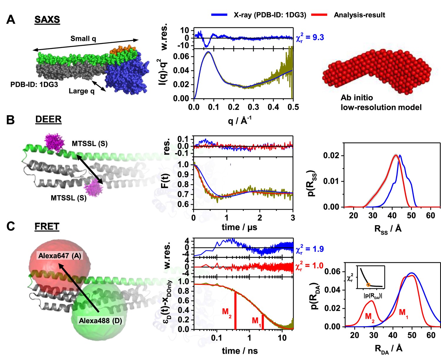
Probing the structure of hGBP1 in solution experimentally.
The left panels illustrate the characteristic properties probed by the experiments: (A) small angle X-ray scattering (SAXS), (B) double electron-electron resonance spectroscopy (DEER), and (C) Förster resonance energy transfer spectroscopy (FRET). In general, all middle panels display representations of the experimental data (dark yellow curves). The right panels show model-free analysis (red). Predicted experimental data based on a full-length X-ray crystal structure (PDB-ID: 1DG3) are shown in blue. To the top of the experimental curves, either data noise weighted, w.res., or unweighted residuals, res., are shown (middle panels). DEER and FRET experiments sense distances between labels that are flexibly coupled to specific labeling sites (exemplified for the double cysteine variant Q344C/A496C). The time-dependent responses of the sample (middle) inform on the inter-label distance distributions (right panels). The recovered distance distributions are compared to structural models by simulating the spatial distribution of the labels around their attachment point (left panels). The spatial distributions of the MTSSL-labels (B, left), as well as the donor and acceptor dye (C, left), are shown in magenta, green, and red, respectively. All distances resolved by EPR and FRET are compiled in Appendix 1—table 1 (A) Left: In SAXS the scattered intensity I(q) is measured as a function of the scattering vector q. Middle: For better illustration, I(q) is presented in a Kratky-plot. The data are deposited in SASBDB (ID: SASDDD6). Right: SAXS ab initio bead modeling determines an average shape of hGBP1 in solution. (B) Left: The DEER experiments measured the dipolar coupling between two MTSSL spin-labels (magenta). Middle: DEER-traces, F(t), analyzed by Tikhonov regularization (red curve). Right: Recovered inter-spin distance distributions, p(RSS). (C) Left: FRET experiments measure the energy transfer from a donor fluorophore (Alexa488, green) to an acceptor fluorophore (Alexa647, red). Middle: Fluorescence intensity decays of the donor analyzed by the maximum entropy method (MEM) recover donor-acceptor distance distributions, p(RDA). The inset displays the L-curve criterion of the MEM reconstruction for the presented data set. The FRET-induced donor decay, εD(t), represents the fluorescence decays (Peulen et al., 2017). εD(t) is corrected for the fraction of FRET-inactive molecules, xDOnly. The shape of εD(t) reveals characteristic times (labeled M1 and M2) that correspond to peaks in p(RDA). Right: Recovered inter-label distance distributions for FRET.
Figure 2—figure supplement 1

Small-angle X-ray scattering measurements on the nucleotide-free hGBP1.
(A) Measured SAXS data of hGBP1 at different protein concentrations. The scattering curves are not normalized by the protein concentration. (B) Structure factor of the 29.9 mg/mL solution extracted from the SAXS data. The structure factor is obtained by the background corrected SAXS curves at highest concentration scaled through division by the form factor (empty circles). The fitted structure factors according to the Percus-Yevik structure factor include the correction for the protein asymmetry factor beta (full line) (Wertheim, 1963; Kotlarchyk and Chen, 1983). For comparison, the uncorrected structure factor without asymmetry factor is given (stitched line). Data are averaged at larger wave vectors to reduce noise.
Figure 2—figure supplement 2

DEER-spectroscopy on a network of MTSSL spin-labeled pairs of the hGBP1 resolves pairwise inter-label distance distributions.
(A) At the top, the network of spin-labeled hGBP1 is shown superposed to a crystal structure of hGBP1. A rotamer library analysis (RLA) simulates for the crystal structure (PDB-ID: 1DG3), the FRET major state (M1), the minor state (M2) inter-spin distance distributions. To the left, experimental background corrected DEER-traces and simulated DEER-traces based on a RLA of different structural models; to the right, inter-spin distance distribution as determined by Tikhonov regularization of the experimental DEER-trace. (B) Parametrization of the EPR-MTSSL label for accessible volume calculations. Top the distance distributions for the spin-pair N18C/Q577C of the hGBP1 crystal structure (PDB-ID: 1DG3) as calculated by the MTSSL-Wizard (Hagelueken et al., 2012) is overlaid by the distance distribution as calculated by accessible volume calculations with the parameter set as provided below. For visual comparison, the rotamers are overlaid with the accessible volume calculated for the labeling position N18C. To parameterize the MTSSL label, we used the variant N18C/Q577C as reference and optimized the simulated linker-length, the label-radius and the linker-width until the distance distribution as determined by the AV-calculations agrees best with the distance distributions as determined by the MTSSL-Wizard (Hagelueken et al., 2012) and MMM (Polyhach, Bordignon et al.). The best agreement was found using a linker-length of 8.5 Å, a linker-width of 4.5 Å and a label-radius of 4.0 Å. All rigid body dockings were performed using this parameter set.
Figure 2—figure supplement 3
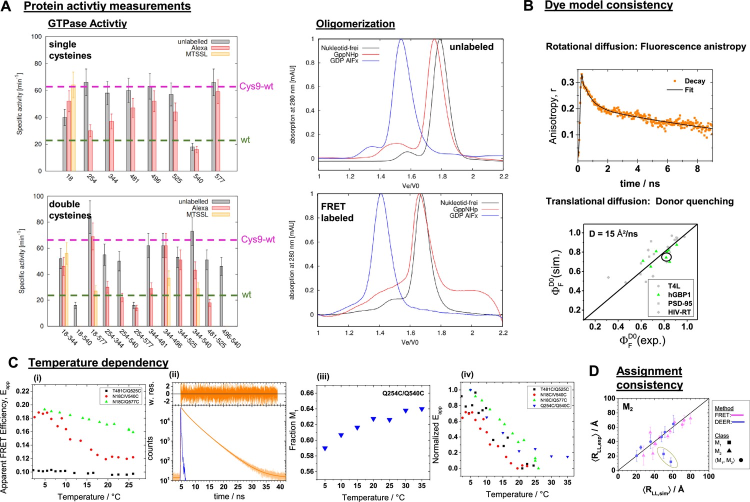
Quality controls for labeling based methods.
(A) Assessment of the labeling on the protein activity by comparison of the GTPase activity (left) and the self-oligomerization of hGBP1 (right). The effect of labeling on GTPase activity of hGBP1 as measured by the specific activities of 1µM single cysteine hGBP1 mutants at 25°C, either unlabeled or modified by Alexa488 or MTSSL at their free cysteines. Specific activities of the hGBP1 variants labeled by Alexa488 and Alexa647. The effect of the labels on the oligomerization of hGBP1 was assessed by size exclusion chromatography of 20 µM of unlabeled (top, right) and double labelled hGBP1 Cys9 (bottom, right) in the presence of 150–200 µM GppNHp or GDP AlFx or in the absence of any nucleotide. (B) The fluorescence properties of the dye were studied by time-resolved anisotropies and dynamic quenching. The donor Alexa488 was predominantly freely rotating. This is highlighted by the fast-initial decay of the time-resolved anisotropy, r(t). (C) Temperature dependent FRET measurements: (i) apparent FRET efficiency ( and are the measured (uncorrected) green and red fluorescence intensities) as measured on a steady-state fluorometer. (ii) Time-resolved fluorescence decay of the hGBP1 variant Q254C/Q540C for a temperature of 35°C. (iii) Temperature dependence of the population of the state M1 for the variant Q254C/Q540C as determined by an analysis of the associated time-resolved fluorescence decays. (iv) Normalized changes of the fluorescence observables in dependence of the temperature. (D) A consistency analysis reveals that two DEER datasets (encircled in yellow) resolve M1 instead of an averaged state of the two states, . The deviation between the simulated and the experimental observables beyond the noise of the other measurements identify two distances assigned to M2 as misassignment.
Figure 3 with 5 supplements
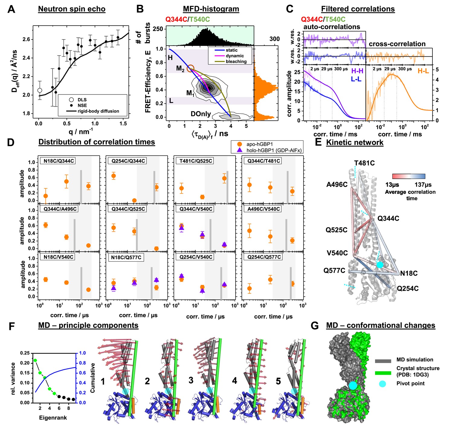
Conformational dynamics of hGBP1 studied by neutron spin echo (NSE), single molecule (sm) FRET with multi-parameter fluorescence detection (MFD), and molecular dynamics (MD) simulations.
(A) Effective diffusion coefficients of hGBP1, Deff, determined by NSE and dynamic light scattering (DLS) compared to a model describing only the rigid body translational and rotational diffusion as a function of the scattering vector, q. The agreement of the experimental and calculated diffusion coefficients demonstrates insignificant shape changes on fast time scales up to 200 ns. (B) Two-dimensional single-molecule histogram of the absolute FRET-efficiency, E, and the average fluorescence weighted lifetimes of the donor in the presence of FRET, 〈τD(A)〉, of the double cysteine variant Q344C/V540C. One-dimensional histograms are projections of the 2D histogram. The color of the variant’s name indicates the location of the donor (green) and acceptor (red) determined by limited proteolysis and time-resolved anisotropies. The static-FRET line (blue) relates E and 〈τD(A)〉 for static proteins. The dynamic FRET line (magenta) describes molecules that change their conformation from M1 to M2 (brown circle) and vice-versa while being observed. The 〈τD(A)〉- E diagrams of all variants are compiled in Figure 3—figure supplement 2. M1 and M2 were identified by eTCSPC (Appendix 1—table 1) and sub-ensemble TCSPC (Figure 3—figure supplement 3, Appendix 1—table 5). Molecules in M2 with bleaching acceptors are described by a bleaching line (dark yellow) that describes the transitions from M2 to the donor only population (DOnly). Photons of molecules in the H and L area (H - high FRET, L - low FRET) were used to generate filters for filtered FCS (fFCS). (C) fFCS species autocorrelation functions (sACF) and species cross-correlation function (sCCF) of the variant Q344C/T540C (semitransparent lines) and corresponding model functions (solid lines) (Materials and Methods, Equation 17). The fFCS model parameters were determined by a global analysis of all 12 FRET-pairs (Figure 3—figure supplement 4) and revealed three correlation times (vertical dotted lines). The weighted residuals are shown to the top. The filter setting for fFCS of all samples and the fit results are compiled in Appendix 1—table 6. (D) Amplitudes of the fitted fFCS correlation times of the GTP free apo- (orange circles) and GDP-AlFx bound holo-state (violet triangles) (values see Appendix 1—table 6). The average correlation times for the variants are shown as gray vertical lines. The gray boxes highlight the minimum and maximum of the average correlation times. (E) The average correlation times of the apo-state are mapped color-coded to a crystal structure (PDB-ID: 1DG3). Sections of the five rigid elements are displayed by cyan dashed lines. (F) Principle components analysis (PCA) of molecular dynamics (MD) and accelerated molecular dynamics (aMD) simulations (Materials and methods). The LG domain, the middle domain, and α12, and α13 are colored in blue, gray, green, and orange, respectively. The red arrows indicate the direction of the motion (scaled by a factor of 1.5 for better visibility). The semi-transparent cyan circle corresponds to a pivot point. The first five principal components (PCs), sorted by the magnitude of the eigenvalues, contribute to 60% of the total variance of all simulations. (G) Superposition of a MD trajectory frame (gray) deviating the most in RMSD (~8 Å) from the crystal structure (green). Both structural models were aligned to the LG domain.
Figure 3—figure supplement 1
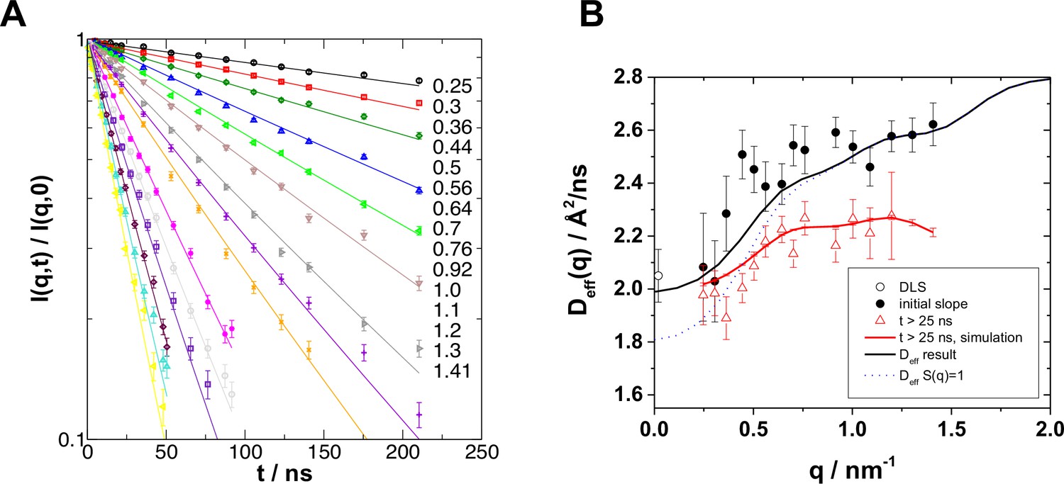
Neutron spin echo spectroscopy (NSE) on the hGBP1 resolves internal dynamics on the nanosecond timescale.
(A) Intermediate scattering function as measured by NSE with fits according to the rigid body models. The numbers to the right show the respective wave-vectors from top down with q in nm-1. (B) Effective diffusion coefficients determined by NSE together with rigid body diffusion calculated from the protein structure. Circles and black line correspond to values derived from the initial slope of the NSE spectra and for rigid body diffusion at infinite dilution. The strong q-dependent increase is entirely due to the elongated shape of the protein. Triangles and red line correspond values obtained from exponential fits to the NSE spectra and to theoretical curves (Materials and Methods, Equation 9) without internal dynamics for t>25 ns. It is evident that rigid body diffusion includes a fast component that is visible at short times below 25 ns.
Figure 3—figure supplement 2
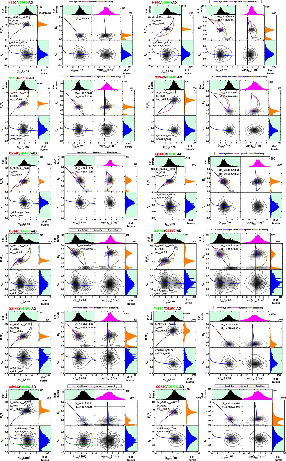
Single-molecule fluorescence measurements.
Multi-parameter fluorescence detection histograms of different variants of Alexa488 and Alexa647 labeled human guanylate binding protein 1. The dashed blue lines are either static FRET-lines (see Materials and methods) considering linker broadening (top panels) or Perrin-equations for a dye with two rotational correlation times (Appendix 2, Equations 21 and 22). x1 and x2 refer to the fraction of fast and slow rotating dyes, respectively. For variants with states of different FRET efficiencies, dynamic FRET-lines connecting these states are shown as magenta solid line. The dark-yellow lines describe the acceptor bleaching from high-FRET states. The data are displayed in histograms of the donor-acceptor fluorescence intensity-ratio, FD/FA, the steady-state transfer-efficiency, ES, and the mean fluorescence averaged lifetime of the donor in the presence of the acceptor ⟨τD(A)⟩F. The variance of the donor-acceptor lifetime var(τDA) was calculated for every detected fluorescence burst. The color of the FRET-pair name indicated the most probable position of the donor (green) and acceptor dye (red); as inset the fluorescence quantum yield of the acceptor ΦF,A and the donor ΦF,D are shown. The fraction of the acceptor Alexa647 in trans-conformation, atrans, was determined by FCS and is shown as inset.
Figure 3—figure supplement 3
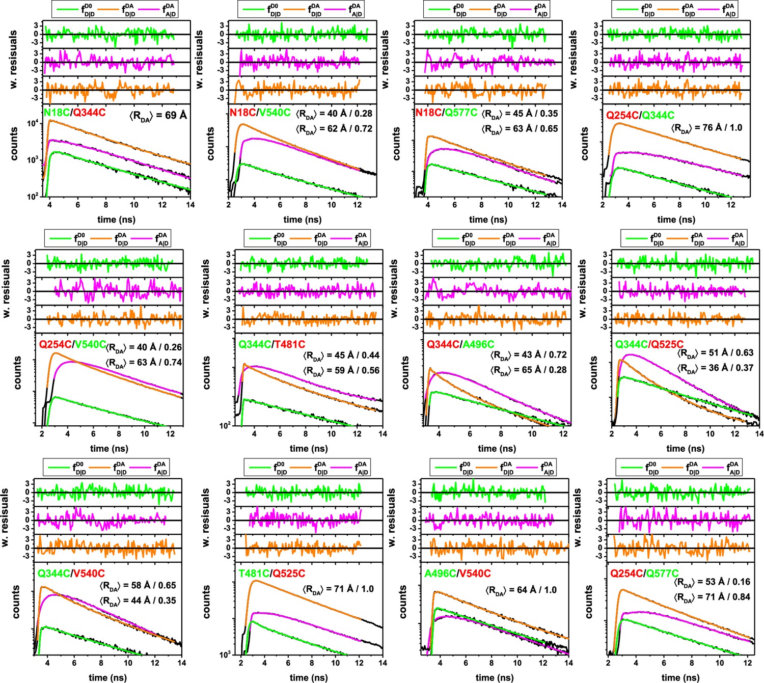
Sub-ensemble fluorescence decays of single-molecule FRET measurements on different FRET-labeled (Alexa488, Alexa647) variant of hGBP1.
Considering the distinct fluorescence species and acquired data, the fluorescence decays of the 12 samples are display in the following colors: Green (, donor fluorescence of the donor-only population D0 of the respective sample, the donor-only population was selected by the acceptor intensity); Orange (, donor fluorescence of the FRET population DA, that is donor in the presence of the acceptor); Magenta (, FRET-sensitized acceptor of the FRET population DA). The fluorescence decays were jointly analyzed by model (Materials and methods, Equations 10–15) with a weighted combination of normal distributed donor-acceptor distances. The mean and the fractions of the normal distributions are reported by the insets, for example, the variant Q254C/Q577C was described by two normal distributions, with average distances of 53 Å and 71 Å with fractions of 0.16 and 0.84, respectively. All fit results are compiled in Appendix 1—table 5.
Figure 3—figure supplement 4
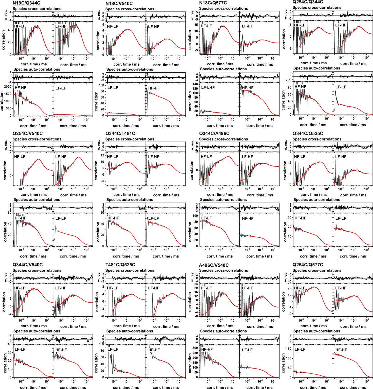
Global analysis of filtered fluorescence correlation spectroscopy of FRET-labeled variants for the hGBP1 probing its internal dynamics from µs to ms.
The model function (red) line is a global (single) model for all depicted fFCS curves. In the MFD histograms high FRET, H, and low FRET, L, species were identified to generate a variant specific set of filters, that are compiled in Appendix 1—table 6. These filters were used to calculate two species cross-correlation functions, sCCFs, and two species autocorrelation functions, sACFs (Materials and methods). For every variant the sCCFs and the sACFs are shown to the top and bottom, respectively. The sACFs and the sCCFs of all variants were analyzed by a global model (red lines, Materials and methods, Equations 17–19) with three correlation times. The weighted residuals of the model and the data are shown to the top of the sACFs and the sCCFs. The displayed correlation curves correspond to the fluorescence intensity weighted average correlation curves obtained by subsetting the measurement. The fluorescence intensity weighted averages correspond to the displayed mean correlation amplitudes of the individual correlation channels. The fit results are compiled in Appendix 1—table 6.
Figure 3—figure supplement 5
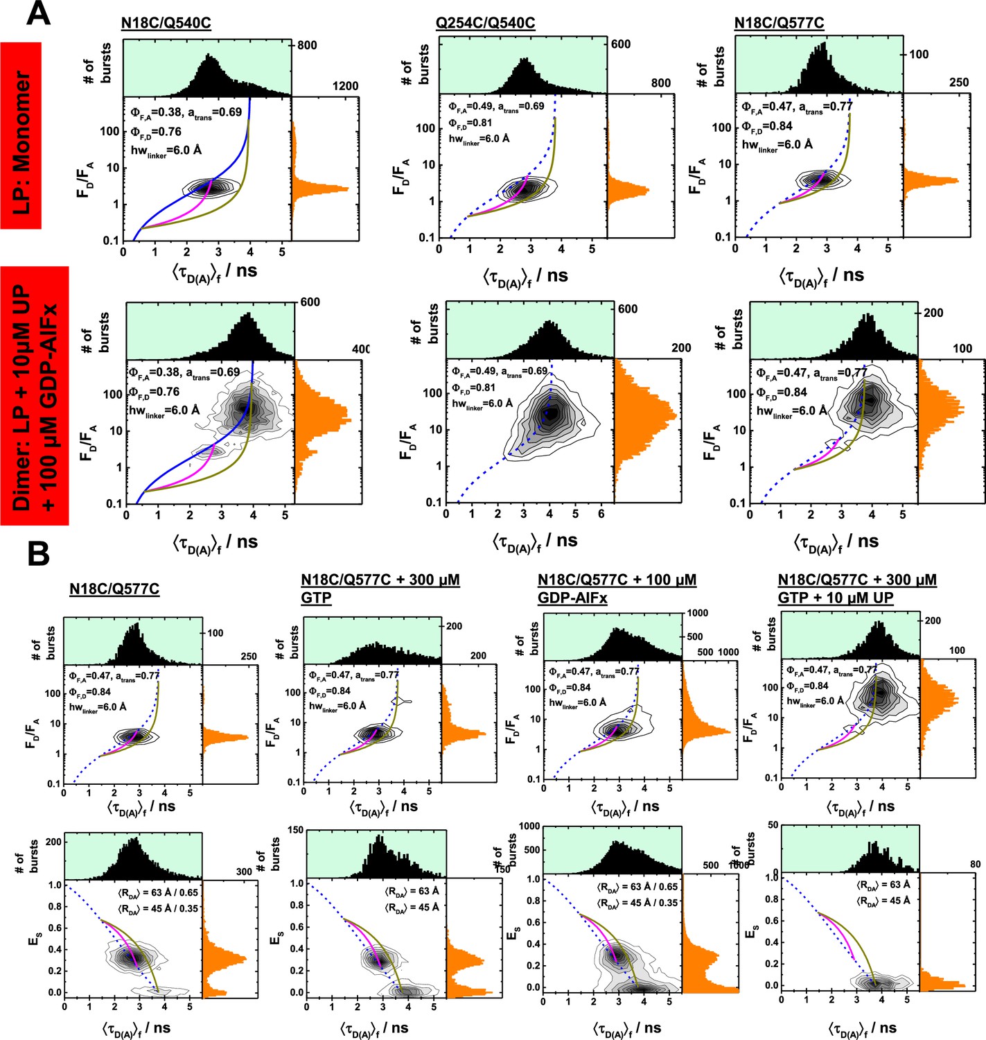
Single-molecule fluorescence measurements under dimer conditions and in the presence of nucleotides.
(A) Multiparameter single-molecule fluorescence measurements of a set of comparable hGBP1 variants that is weakly affected in their GTP hydrolysis to different extent by the introduced mutations and labels. The labeling positions N18C and Q254C are on opposing sites of the molecule. LP and UP refer to labeled protein and unlabeled protein, respectively. In the presence of UP (10 µM) and GDP-AlFx (100 µM) hGBP1 forms a dimer and undergoes significant conformational changes. These conformational changes were detected for the variants with weakly (N18C/Q577C) and variants stronger affected in their GTP hydrolysis (Q254C/Q540C) & (N18C/Q577C). The mutation Q577C has for the labeled and the unlabeled hGBP1 no effect on the specific activity. The mutation Q540C affects GTP hydrolysis activity of the labeled and the unlabeled hGBP1 equally strong. The mutation Q254C affects the GTP hydrolysis activity only the presence of a dye. (B) Control measurements of the variant N18C/Q577C to study the effect of GTP binding on hGBP1. Under single-molecule conditions (pM concentration) the intensity-based FRET indicators (FD/FA and the FRET efficiency, E) are independent on the presence of the substrate GTP. In the presence of GTP and hGBP1 at micromolar concentration oligomerization / dimerization occurs and hGBP1 undergoes a conformational change highlighted by a change of the FRET indicators.
Figure 4 with 2 supplements
Integrative modeling workflow and structure validation.
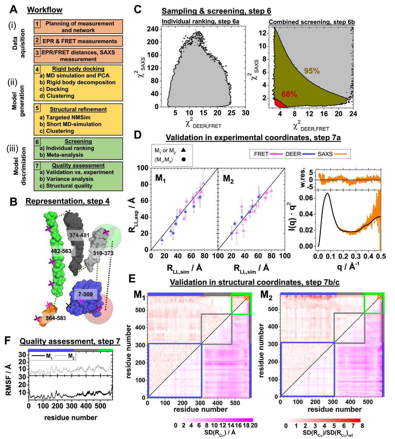
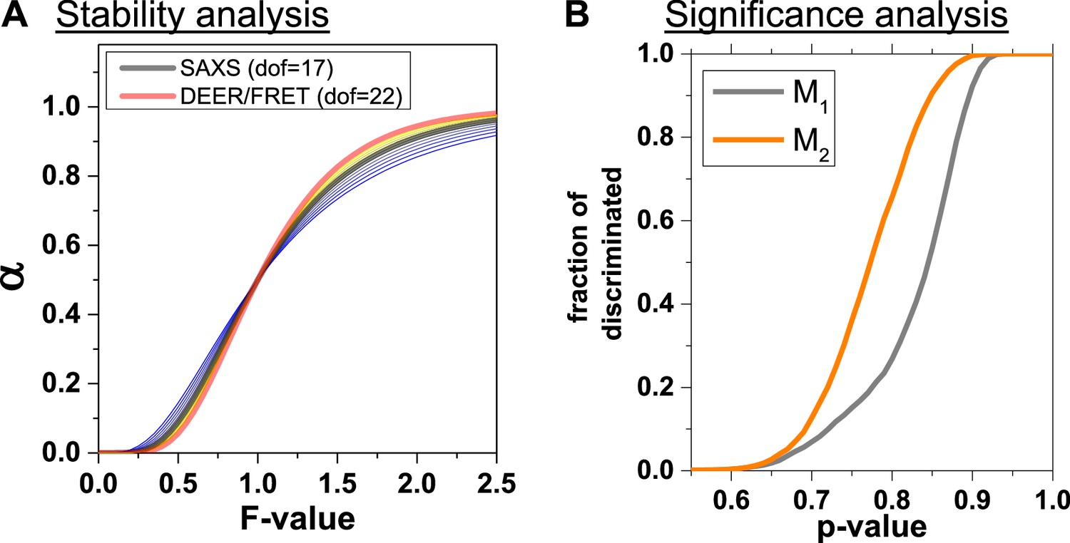
A detailed description and the used data can be found in Appendix 3. (A) The workflow combines rigid body docking (RBD), structural refinements, and molecular dynamics (MD) simulations. Rigid bodies (RBs) are identified by MD simulations and principal components analysis (PCA) (Materials and methods). (B) RBD representation of hGBP1: LG-domain (blue), the middle domain (gray), helix α12 (green), helix α13 (orange). The numbers correspond to the RB amino acid ranges. The crosses mark the FRET (black) and the EPR (magenta) labeling positions. The RBD considers the label distribution illustrated for a FRET pair by semi-transparent green (donor) and red (acceptor) surfaces. (C) Left: outline of (Appendix 3, Equation 27) and (Appendix 3, Equation 28) for all (M1, M2) pairs of structures (left). Confidence levels of the meta-analysis (Materials and methods, Equation 20) that discriminates (M1, M2) pairs (right). Red and dark yellow regions correspond to p-values smaller than 0.68 and 0.95, respectively. (D) Experimental validation of the best pair of structures. Comparison of experimental (for DEER and for FRET ) and modeled label distances (for DEER and FRET ). Specific symbols display label distances for label pairs with distinct (▲) and equal (●) values for M1 and M2, respectively (see Appendix 1—table 1). For SAXS the scattering curve (black line) of the structure pair (M1, M2) is compared to the experimental data (orange line) by the weighted residuals to the top. (E) The standard deviation, SD, of the pairwise Cα-Cα distance of the experimental ensemble with a p-value <0.68 (lower triangles) highlights the structural uncertainty. normalized by the computed by the experimental uncertainty validates the structures. (F) Root mean square fluctuations (RMSF) of the Cα atoms of structures with a p-value <0.68 are displayed for the globally aligned ensemble.
Figure 4—figure supplement 1
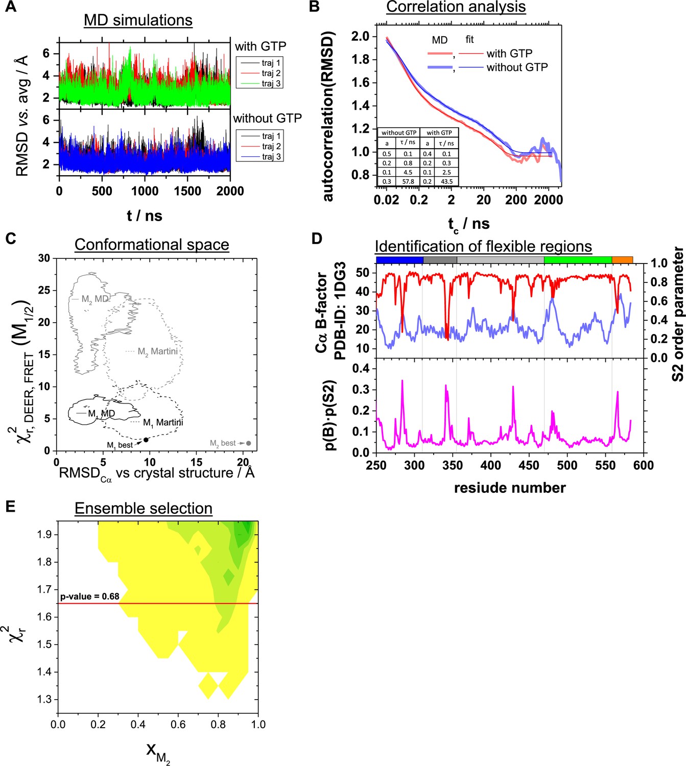
Analysis of molecular dynamics simulations, conformational space, identification of flexible regions, ensemble selection.
(A) Root mean squared deviation (RMSD) vs. the average structure of three repeats of 2 µs MD simulations in the presence and absence of GTP bound to the binding pocket of the LG domain. (B) Autocorrelation analysis of the RMSDs. The autocorrelation function of the RMSD vs. the average structure of the MD simulations in the presence (red) and absence (blue) of GTP are shown as light-colored thick lines. tc is the correlation time. The darker colored red and blue lines correspond to a multiexponential model (). The amplitudes ai and the characteristic times are given in the table shown as an inset. (C) Assessment of the conformers within the conformational space covered by MD simulations using FRET- and EPR-data (Appendix 1—table 1). We evaluated the conformers obtained by multi-resolution MD simulations all-atom MD and coarse-grained MD with the Martini force field of Barz et al., 2019 using our FRET positioning and screening (FPS) toolkit (Kalinin et al., 2012) to compute the quality parameter (Appendix 3, Equation 28). The structural features of the conformers are described by the measure, RMSDCα versus the hGBP1 crystal structure (PDB-ID: 1DG3). For comparison, we added the parameters of the best representative conformers for M1 and M2 obtained by our integrative structural modeling (Figure 5). (D) To the top the crystallographic B-factors of the Cα atoms (PDB-ID: 1DG3) and the NH S2 order parameters calculated from the MD simulations are shown. The bottom graph illustrated the product of the B-factor normalized to the range of (0,1] and the NH S2 order parameter. (E) Ensemble selection. The fitted fractions of the conformer M2, xM2, for all combinations (M1, M2) generated by rigid body docking (RBD) using the DEER and FRET constraints are shown in dependence of the reduced sum of the squared deviation, , in a 2D histogram. The red line corresponds to a p-value of 0.68. Pairs of structural models above the red line are discriminated.
Figure 4—figure supplement 2
Analysis of structure generation and discrimination.
(A) Cumulative probability α that for a given F-value a proposed structural model is significantly worse than the best-found structural model. The experimental degrees of freedom (dofd,SAXS) for SAXS was varied from 11 to 24 taking the values 11, 12, 13, 14, 15, 16, 17, 18, 20, 22, 24 with colors varying from blue to yellow. The cumulative probabilities were calculated using the best model as a reference () and an estimate of dofm ~10 for the degrees of freedom of the model (Appendix 3, Equation 29). The dofd,SAXS was varied to assess the influence of the relative weights of DEER, FRET and SAXS (Materials and methods, Equation 20). (B) Fraction of discriminated structures vs. p-value of discriminating a pair of structure from the best structure.
Figure 5 with 1 supplement
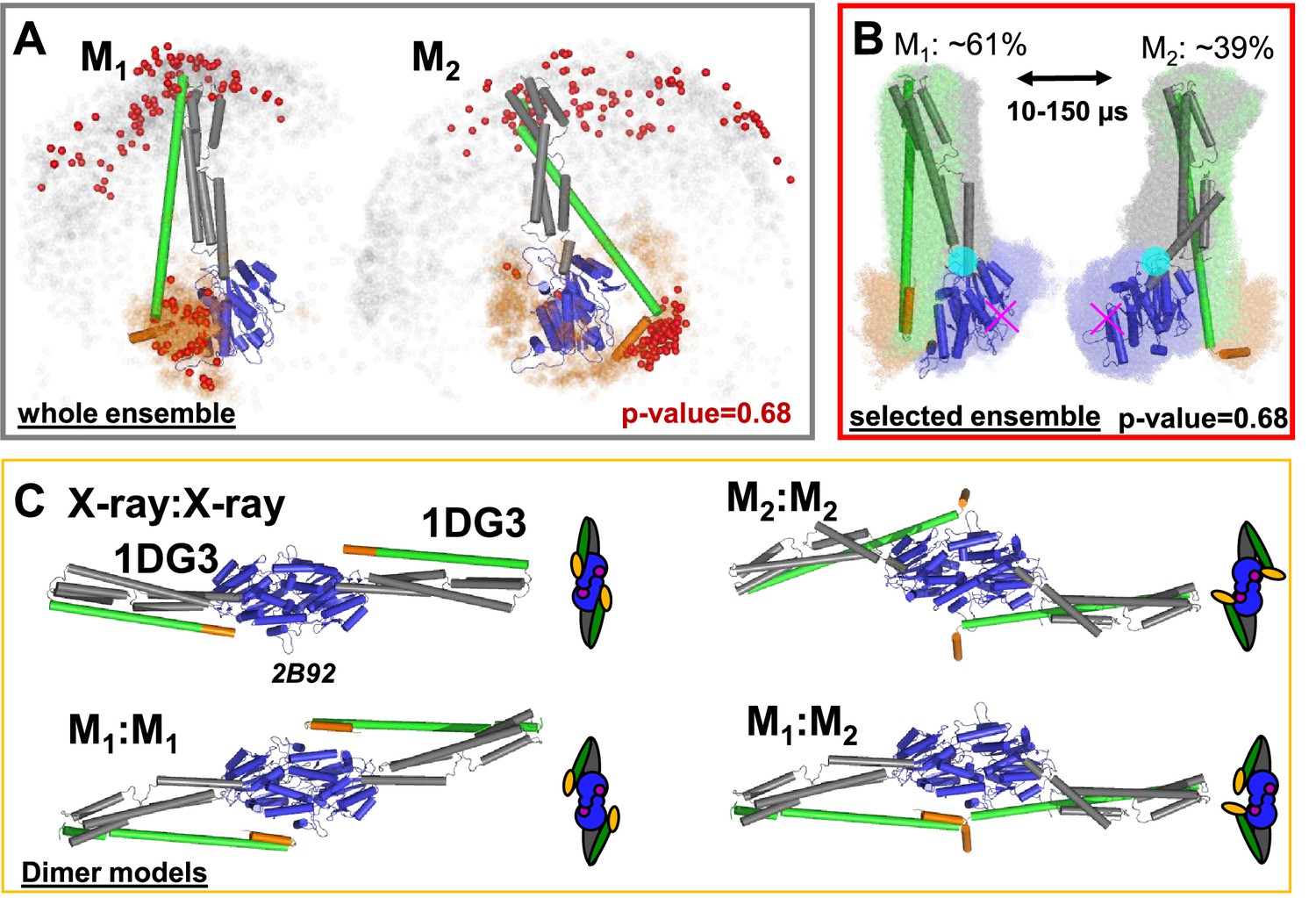
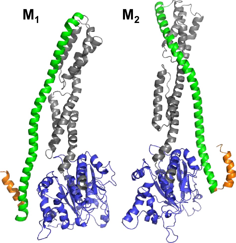
Selected conformers and corresponding dimer models based on integrative modeling structures using of DEER, FRET, and SAXS data.
(A) All structures for M1 and M2 were aligned to the LG domain and are represented by orange and gray dots, indicating the Cα atoms of the amino acids F565 and T481, respectively. The structures best agreeing with all experiments are shown as cartoon representation (ribbon presentation see Figure 5—figure supplement 1). Non-rejected structures (p-value = 0.68, Figure 4—figure supplement 1E) represented by red spheres. The ensemble has been at deposited at PDB-Dev with the ID: PDBDEV_00000088. (B) Global alignment of all selected structures (p-value = 0.68). In the center, the structures best representing the average of the selected ensembles are shown. The transition from M1 to M2 (average correlation times 10–150 µs) can be described by a rotation around the region connecting the LG with the ligand binding site (magenta cross) and the middle domain (cyan circle). (C) Potential hGBP1:hGBP1 dimer structures constructed by superposing the head-to-head interface of the LG domain (PDB-ID: 2B92) to the full-length crystal structure (1DG3). The LG and middle domain are colored in blue and gray, respectively. Helices α12 and α13 are colored in green and orange, respectively.
Figure 5—figure supplement 1
Selected conformers models based on integrative modeling structures using of DEER, FRET, and SAXS data.
(A) The pair of structural models (M1, M2) selected from the structural ensemble generated by DEER- and FRET-measurements best corresponding to the SAXS scattering data is shown in a cartoon representation. Both structural models are aligned to the LG domain.
Figure 6
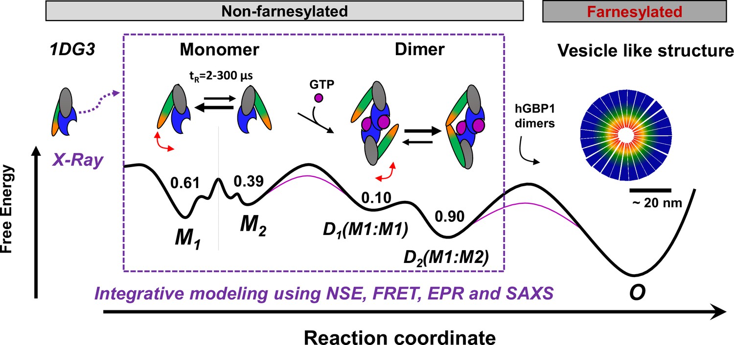
Potential oligomerization pathways of the human guanylate binding protein 1 (hGBP1) summarizing current experimental findings (Kravets et al., 2012, Vöpel et al., 2014; Kravets et al., 2016; Shydlovskyi et al., 2017).
In the presence and absence of a nucleotide, hGBP1 is in a conformational exchange with a Pivot point between LG and middle domain resulting in at least two conformational states M1 and M2 with a correlation time of 2–300 µs. Binding of a nucleotide to the LG domain activates hGBP1 for dimerization. After hGBP1 dimerization via the LG domains conformational changes of the middle domains and the helices α12/13 lead to an association of both helices α13. The species fractions for respective populations are given as numbers on top of the wells of a schematic energy landscape (black line). The substrate GTP lowers the activation barrier (red line). Under turn-over of GTP, farnesylated hGBP1 further self-assembles to form highly ordered, micelle-like polymers.
Tables
Appendix 1—table 1
Inter-label distance analysis of DEER measurements, ensemble fluorescence decays of the donor (eTCSPC), and residual donor fluorescence anisotropies.
Average distances between the spin-labels are referred to as . The width of the inter-spin distance distribution is w. The center values of the donor-acceptor distance distribution correspond to and for the states, M1 and M2, respectively. The average donor-acceptor distance and the inter-spin distance simulated for the full-length crystal structure of hGBP1 (PDB-ID: 1DG3) are and , respectively, with corresponding distribution widths w. The uncertainty estimates of central distance of a state determined by FRET is .
| Category | DEER(a) | DEER(a) | ensemble FRET(b) | ensemble FRET(b) | Fluorescence Anisotropy(e) | ||||
|---|---|---|---|---|---|---|---|---|---|
| Type | Experiment | Simulation(c) | Experiment | Simulation(d) | Experiment | ||||
| State | Average over all states | Crystal (PDB-ID: 1DG3) | M1 | M2 | Crystal (PDB-ID: 1DG3) | Donor Alexa488 | |||
| Joint species fractions x1, x2 | 0.61 | 0.39 | |||||||
| Variant | / Å | () / Å | / Å | () / Å | ± / Å | ± / Å | / Å | () / Å | |
| N18C/Q344C | 64.6 | (12.2) | 66.5 | (9.5) | 73.6±8.6 | 67.0±5.5 | 72.4 | (12.1) | 0.15 |
| N18C/V540C | 57.8±3.6 | 36.6±2.7 | 63.6 | (8.8) | 0.11 | ||||
| N18C/Q577C | 53.2 | (7.6) | 50.5 | (7.5) | 64.2±4.7 | 47.4±2.8 | 60.1 | (10.5) | 0.15 |
| C225/K567C | 12.0 | (5.5) | 13.0 | (6.5) | |||||
| C225/Q577C | 22.9 | (6.0) | 19.5 | (10.0) | |||||
| Q254C/Q344C | 81.3±16.5 | 72.3±7.8 | 73.9 | (12.2) | 0.13 | ||||
| Q254C/V540C | 63.6±4.6 | 36.8±2.7 | 60.9 | (12.4) | 0.30 | ||||
| Q254C/V577C | 70.8±9.1 | 52.9±7.4 | 73.1 | (8.9) | 0.17 | ||||
| Q344C/T481C | 37.9±2.6 | 54.5±3.3 | 57.6 | (11.2) | 0.11 | ||||
| Q344C/A496C | 40.0 | (9.6) | 42.5 | (10.0) | 48.0±2.9 | 23.5±8.2 | 48.4 | (10.6) | 0.19 |
| Q344C/Q525C | 32.0 | (5.4) | 29.5 | (10.2) | 46.7±2.8 | 20.7±13.3 | 41.5 | (10.7) | 0.30 |
| Q344C/V540C | 46.6 | (6.8) | 43.0 | (14.5) | 59.3±3.8 | 45.5±2.8 | 48.7 | (11.9) | 0.10 |
| T481C/Q525C | 69.6±6.4 | 69.5±6.4 | 71.2 | (11.0) | 0.30 | ||||
| A496C/V540C | 63.6±4.6 | 63.6±4.6 | 66.8 | (11.6) | 0.23 | ||||
| A551C/Q577C | 20.5 | (7.7) | 22.5 | (5.0) | |||||
-
(a) DEER distance distributions for calculation of average inter-spin distances and width were determined by Tikhonov regularization of the experimental DEER-traces (Materials and methods, Equation 6). All data are shown in Figure 2—figure supplement 2.
-
(b) The ensemble fluorescence decays of the donors were jointly analyzed by a quasi-static homogeneous model (Peulen et al., 2017) with two FRET species with the species fractions x1 and x2 as well as a D-only species (Materials and methods, Equations 12; 13) using the donor properties in Appendix 1—table 2 and a Förster radius R0=52 Å. Moreover, the model accounted for the distance distribution with a typical width of 12 Å caused by the flexible dye-linkers (Materials and methods, Equation 13). The reported uncertainty estimates, indicated by ±, include statistical uncertainties, potential systematic errors of the references, uncertainties of the orientation factor determined by the anisotropy of donor samples, and uncertainties of the AVs due to the differences of the donor and acceptor linker length (Appendix 2). The individual uncertainty components are listed in Appendix 1—table 4. Reference measurements of single D and A labeled variants are summarized in Appendix 1—table 2, respectively. The distances recovered by eTCSPC and seTCSPC (Appendix 1—table 5), respectively, agree nicely within the distinct precision of each data set.
-
(c) For EPR-DEER the inter-spin distance distribution was calculated by a rotamer library analysis.
-
(d) The inter- fluorophores distance distribution and the corresponding average distance and width were calculated by accessible volume simulations (Kalinin et al., 2012).
-
(e) Residual anisotropies of Alexa488 in FRET labeled (Alexa488, Alexa647) variants of hGBP1 determined by an analysis of the MFD histograms using a Perrin equation for a bi-exponential anisotropy decay (Appendix 2, Equation 21). All data are shown in Figure 3—figure supplement 2.
Appendix 1—table 2
Fluorescence lifetimes of Alexa647 and Alexa488 coupled to single cysteine variants of hGBP1 determined from ensemble TCSPC.
Fluorescence lifetimes, τ, with corresponding species fractions, x, of Alexa647- and Alexa488-maleimide coupled to different single cysteine variants of the hGBP1 determined by an analysis of the fluorescence intensity decays measured by ensemble TCSPC.
| Variant | Alexa647(a) | Alexa488(a) | ||||||||||||
|---|---|---|---|---|---|---|---|---|---|---|---|---|---|---|
| Alexa647(a) | Alexa647(a) | Alexa647(a) | Alexa647(a) | Alexa488(a) | Alexa488(a) | Alexa488(a) | ||||||||
| / ns | (x1) | / ns | (x2) | / ns | (x3) | / ns(b) | ΦF,A(c) | / ns | (x1)(a) | / ns | (x2) | / ns(b) | ΦF,D(c) | |
| N18C | 1.85 | (0.39) | 1.22 | (0.49) | 0.10 | (0.12) | 1.33 | 0.40 | 4.15 | (0.82) | 1.35 | (0.18) | 3.65 | 0.82 |
| Q254C | 2.23 | (0.58) | 1.42 | (0.42) | 1.89 | 0.57 | 3.60 | (0.69) | 0.53 | (0.31) | 2.65 | 0.59 | ||
| Q344C | 2.06 | (0.58) | 1.09 | (0.42) | 1.75 | 0.52 | 3.80 | (0.94) | 1.00 | (0.06) | 3.63 | 0.81 | ||
| T481C | 1.89 | (0.43) | 1.32 | (0.57) | 1.57 | 0.43 | 3.78 | (0.93) | 1.07 | (0.07) | 3.59 | 0.81 | ||
| A496C | 1.21 | (0.43) | 1.88 | (0.57) | 1.59 | 0.48 | 3.89 | (0.84) | 1.14 | (0.16) | 3.44 | 0.77 | ||
| Q525C | 1.93 | (0.65) | 1.08 | (0.35) | 1.63 | 0.49 | 3.51 | (0.80) | 0.66 | (0.20) | 2.94 | 0.66 | ||
| V540C | 2.33 | (0.65) | 1.43 | (0.35) | 2.02 | 0.60 | 4.00 | (0.85) | 1.86 | (0.15) | 3.67 | 0.82 | ||
| Q577C | 2.06 | (0.49) | 1.42 | (0.51) | 1.73 | 0.52 | 4.15 | (0.91) | 1.49 | (0.09) | 3.91 | 0.88 | ||
-
(a) The number of fluorescence lifetime components corresponds to the minimum number required to sufficiently describe the experimental data, as judged by a criterion (Materials and methods, Equation 10).
-
(b) ⟨τ⟩x is the species weighted average fluorescence lifetime .
-
(c) is the fluorescence quantum yield of the fluorescent dye species estimated by the species averaged fluorescence lifetime ⟨τ⟩x using ⟨τ⟩x and of the free dyes as a reference; (Alexa647, ⟨τ⟩x=1.0 ns, ) (Alexa488, ⟨τ⟩x=4.1 ns, ).
Appendix 1—table 3
Fluorescence quantum yields of donor and acceptor dye in FRET samples under single-molecule measurement conditions to compute the FRET-lines in the E-diagrams (Figure 3—figure supplement 2).
| FRET sample | Donor(a) | Acceptor | ΦF,D (b) | ΦF,A(c) | atrans(d) |
|---|---|---|---|---|---|
| N18C/V344C | V344C | N18C | 0.83 | 0.38 | 0.75 |
| N18C/V540C | V540C | N18C | 0.76 | 0.38 | 0.69 |
| N18C/Q577C | N18C | Q577C | 0.84 | 0.47 | 0.77 |
| Q254C/Q344C | Q344C | Q254C | 0.82 | 0.50 | 0.70 |
| Q254C/W540C | Q540C | Q254C | 0.81 | 0.49 | 0.69 |
| Q344C/T481C | T481C | Q344C | 0.81 | 0.40 | 0.73 |
| Q344C/A496C | A496C | Q344C | 0.85 | 0.37 | 0.73 |
| Q344C/Q525C | Q344C | Q525C | 0.81 | 0.47 | 0.76 |
| Q344C/V540C | V540C | Q344C | 0.82 | 0.43 | 0.65 |
| T481C/Q525C | T481C | Q525C | 0.81 | 0.41 | 0.67 |
| A496C/V540C | V540C | A496C | 0.87 | 0.38 | 0.65 |
| Q254C/Q577C | Q577C | Q254C | 0.90 | 0.47 | 0.67 |
-
(a) Donor/acceptor position as determined by limited trypsin proteolysis of single labeled reference samples and double labeled FRET sample described by Rothwell et al., 2013.
-
(b) ΦF,D=Fluorescence lifetime of the reference (4.1 ns, ΦF,D=0.9) and correction for triplet amplitude (donor dye FCS measurement at same power).
-
(c) ΦF,A=Fluorescence lifetime reference dye and correction for triplet,
-
(d) atrans fraction of Alexa647 in trans state was estimated as previously described (Widengren et al., 2001; compare Appendix 1—table 2).
Appendix 1—table 4
Combined and individual uncertainty contributions of the average inter-dye distances determined by eTCSPC measurements.
| Variant | State | Combined uncertainty(a) | Statistical uncertainty(b) | Reference uncertainty(c) | Dye simulation(d) | Orientation factor(e) | ||
|---|---|---|---|---|---|---|---|---|
| δ+ | δ- | δstat | δ+,ref | δ-,ref | δAV | δ,κ2 | ||
| N18C/Q344C | (1) | 12.1% | 11.3% | 9.1% | 6.0% | 4.2% | 1.1% | 4.9% |
| N18C/V540C | (1) | 6.3% | 6.3% | 3.1% | 1.2% | 1.1% | 1.4% | 4.5% |
| N18C/Q577C | (1) | 7.4% | 7.3% | 4.6% | 2.3% | 2.0% | 1.2% | 4.9% |
| Q254C/Q344C | (1) | 22.0% | 18.6% | 16.5% | 13.5% | 6.9% | 1.0% | 4.7% |
| Q254C/V540C | (1) | 7.2% | 7.1% | 4.4% | 2.2% | 1.9% | 1.3% | 5.8% |
| Q344C/T481C | (1) | 6.9% | 6.9% | 4.1% | 0.1% | 0.1% | 2.1% | 4.5% |
| Q344C/A496C | (1) | 6.0% | 6.0% | 2.5% | 0.4% | 0.4% | 1.7% | 5.4% |
| Q344C/Q525C | (1) | 6.0% | 6.0% | 2.5% | 0.3% | 0.3% | 1.7% | 6.1% |
| Q344C/V540C | (1) | 6.5% | 6.4% | 3.4% | 1.4% | 1.3% | 1.3% | 4.3% |
| T481C/Q525C | (1) | 9.4% | 9.1% | 6.7% | 4.0% | 3.1% | 1.2% | 6.1% |
| A496C/V540C | (1) | 7.2% | 7.2% | 4.4% | 2.2% | 1.9% | 1.3% | 5.7% |
| Q254C/Q577C | (1) | 13.0% | 12.7% | 11.0% | 4.5% | 3.4% | 1.1% | 5.1% |
| N18C/Q344C | (2) | 8.1% | 7.9% | 5.6% | 3.1% | 2.5% | 1.2% | 4.9% |
| N18C/V540C | (2) | 7.3% | 7.3% | 4.6% | 0.1% | 0.1% | 2.2% | 4.5% |
| N18C/Q577C | (2) | 5.8% | 5.8% | 2.5% | 0.4% | 0.3% | 1.7% | 4.9% |
| Q254C/Q344C | (2) | 10.9% | 10.3% | 8.3% | 5.3% | 3.8% | 1.1% | 4.7% |
| Q254C/V540C | (2) | 7.7% | 7.7% | 4.5% | 0.1% | 0.1% | 2.2% | 5.8% |
| Q344C/T481C | (2) | 5.5% | 5.5% | 2.7% | 0.8% | 0.8% | 1.5% | 4.5% |
| Q344C/A496C | (2) | 34.8% | 34.8% | 34.2% | 0.0% | 0.0% | 3.4% | 5.4% |
| Q344C/Q525C | (2) | 64.6% | 64.6% | 64.2% | 0.0% | 0.0% | 3.9% | 6.1% |
| Q344C/V540C | (2) | 5.4% | 5.4% | 2.6% | 0.3% | 0.3% | 1.8% | 4.3% |
| T481C/Q525C | (2) | 10.0% | 9.7% | 6.7% | 4.0% | 3.1% | 1.2% | 6.1% |
| A496C/V540C | (2) | 7.6% | 7.5% | 4.4% | 2.2% | 1.9% | 1.3% | 5.7% |
| Q254C/Q577C | (2) | 14.0% | 14.0% | 12.9% | 0.7% | 0.7% | 1.5% | 5.1% |
-
(a) The combined uncertainty used to calculate the relative (δ±) and the absolute (Δ±) uncertainties of the inter-dye distances considers the uncertainty of the dye simulations, δAV, the uncertainty of the orientation factor, δ,κ2, the uncertainty of the reference sample, δ±,ref, and the statistical uncertainty determined by the noise of the measurements, δstat (Appendix 2, Equation 23).
-
(b) The statistical uncertainties were estimated by sampling the distances that agree with the experimental ensemble TCSPC data (Appendix 1—table 1).
-
(c) The reference uncertainties were calculated assuming an uncertainty of the reference donor fluorescence lifetime of .
-
(d) The dye simulation error considers the labeling uncertainty of the dye. In accessible volume simulations (AV) for the dye pair Alexa488/Alexa647 this labeling uncertainty results in an expected error of Å (Vöpel et al., 2014).
-
(e) The uncertainty of the distance due to the orientation factor was estimated using a wobbling in a cone model of the dyes using the experimental anisotropies (Appendix 1—table 1).
Appendix 1—table 5
Complementary inter-dye distance analysis of donor and sensitized acceptor fluorescence decays of the FRET-active DA sub-ensemble from single-molecule FRET experiments.
Complementary inter-dye distance analysis of donor and sensitized acceptor fluorescence decays of the FRET-active DA sub-ensemble (seTCSPC) (Figure 3—figure supplement 3) obtained from of single-molecule FRET experiments (Figure 3—figure supplement 2) for different FRET labeled (Alexa488, Alexa647) hGBP1 variants.
The donor and acceptor fluorescence decays were described by a combination of two normal distributed distances with the central distances of of a state. The fractions x1 and x2 correspond to the fraction of the distance and , respectively. xDOnly is the fraction of molecules with no energy transfer to an acceptor. The distances recovered by eTCSPC (Appendix 1—table 1) and seTCSPC, respectively, agree nicely within the distinct precision of each data set.
| hGBP1 variant | / Å | x1 | / Å(a) | x2(a) | xDOnly |
|---|---|---|---|---|---|
| N18C/Q344C | 69.3 | 1.00 | - | - | 0.18 |
| N18C/V540C | 60.0 | 0.50 | 34.1 | 0.50 | 0.37 |
| N18C/Q577C | 63.3 | 0.65 | 45.1 | 0.35 | 0.17 |
| Q254C/Q344C | 76.1 | 1.00 | - | - | 0.21 |
| Q254C/V540C | 63.4 | 0.74 | 39.3 | 0.26 | 0.31 |
| Q344C/T481C | 45.0 | 0.44 | 59.3 | 0.56 | 0.17 |
| Q344C/A496C | 47.0 | 0.77 | 36.0 | 0.23 | 0.45 |
| Q344C/Q525C | 51.5 | 0.63 | 36.1 | 0.37 | 0.40 |
| Q344C/V540C | 57.8 | 0.65 | 43.8 | 0.35 | 0.24 |
| T481C/Q525C | 70.6 | 1.00 | - | - | 0.20 |
| A496C/V540C | 63.9 | 1.00 | - | - | 0.37 |
| Q254C/Q577C | 70.8 | 0.84 | 52.9 | 0.16 | 0.34 |
-
(a) For cases where a single normal distribution was enough to describe the data no second distance and fraction is reported.
Appendix 1—table 6
Filtered fluorescence correlation spectroscopy (fFCS) of all FRET-labeled variants of the human guanylate binding protein 1 analyzed by a global model with joint relaxation times and individual amplitudes Ai.
Selection criteria for the definition of the filters for the high FRET (HF) and low FRET (LF) species.
| Amplitude(a) | Burst selection criteria for fFCS filter generation(b) | ||||||
|---|---|---|---|---|---|---|---|
| hGBP1 variant | HF range, Sg/Sr | LF range, Sg/Sr | |||||
| N18C/Q344C | 0.38±0.09 | 0.50±0.18 | 0.12±0.20 | 0.09 | 2.03 | 5.82 | 13.19 |
| N18C/V540C | 0.18±0.03 | 0.37±0.04 | 0.45±0.06 | 0.10 | 1.00 | 4.00 | 10.80 |
| N18C/Q577C | 0.24±0.06 | 0.41±0.09 | 0.36±0.11 | 0.40 | 1.50 | 3.00 | 26.00 |
| Q254C/Q344C | 0.35±0.09 | 0.00±0.00 | 0.65±0.09 | 0.70 | 1.70 | 2.80 | 5.90 |
| Q254C/V540C | 0.34±0.03 | 0.21±0.05 | 0.45±0.06 | 0.18 | 0.56 | 3.50 | 8.90 |
| Q344C/T481C | 0.24±0.11 | 0.34±0.14 | 0.41±0.18 | 0.10 | 0.60 | 1.60 | 6.30 |
| Q344C/A496C | 0.08±0.03 | 0.30±0.06 | 0.62±0.07 | 0.03 | 0.58 | 1.70 | 22.36 |
| Q344C/Q525C | 0.00±0.05 | 0.45±0.09 | 0.55±0.10 | 0.07 | 0.28 | 2.94 | 8.07 |
| Q344C/V540C | 0.08±0.02 | 0.33±0.07 | 0.59±0.07 | 0.08 | 0.70 | 1.92 | 8.74 |
| T481C/Q525C | 0.58±0.13 | 0.09±0.05 | 0.32±0.14 | 0.60 | 1.52 | 16.27 | 25.40 |
| A496C/V540C | 0.21±0.07 | 0.32±0.17 | 0.47±0.18 | 0.07 | 1.77 | 4.61 | 11.40 |
| Q254C/Q577C | 0.34±0.07 | 0.45±0.11 | 0.21±0.13 | 0.51 | 1.39 | 5.18 | 11.07 |
| Correlation time / µs | 297.6 | 22.6 | 2.0 | ||||
-
(a) The correlation times were determined by a joint/global analysis of fFCS curves (Materials and methods, Equation 19, Figure 3—figure supplement 4). The amplitudes A1, A2, and A3 are variant specific. The uncertainties were determined by a support plane analysis, which considers the mean and the standard deviation of the individual correlation channels determined by splitting the measurements into smaller sets.
-
(b) Filters defining the high FRET (HF) and the low FRET (LF) species were generated by selecting bursts that are within the given ranges. To select high FRET and low FRET bursts the ratio of the green and red signal intensity ratio, Sg/Sr, was used. Sub-ensemble fluorescence decay histograms of the molecules in these ranges were generated and used to calculated filters for fFCS as previously described (Felekyan et al., 2012).
Appendix 3—table 1
Experimental restraints for rigid body docking.
Analysis results of DEER-EPR and FRET eTCSPC. The labels Alexa488, Alexa647, and MTSSL are referred to by D, A, and R1, respectively. The names of the labeling sites report on the location of the dyes and the introduced mutation. For DEER, average inter-label distances and the widths of the inter-spin distance distribution and are reported (Appendix 1—table 1). For FRET, mean distances (Appendix 1—table 1) and uncertainties of the mean are reported (Δ+and Δ-) (Appendix 1—table 4). The measurements are grouped into three classes. Class (I) informs on M1 and M2 by two distinct distances. Class (II) informed on M1. In class (III) measurements M1 and M2 were not resolved into separate states. The simulated average label-to-label distances correspond to the distances of the pair of structures (M1, M2) best agreeing with SAXS, DEER, and FRET combined (Figure 5—figure supplement 1).
| # | Technique | Experiment | Experiment | Simulation | Class | |||||
|---|---|---|---|---|---|---|---|---|---|---|
| Labelling site(a) | M1 | M2 | M1 | M2 | ||||||
| 1 | 2 | / Å | (Δ+; Δ-) / Å | / Å | (Δ+; Δ-) / Å | / Å | ||||
| 1 | FRET | Q344CD | N18CA | 73.6 | (8.9; 8.3) | 67.0 | (5.6; 5.4) | 73.9 | 62.3 | (I) |
| 2 | FRET | V540CD | N18CA | 57.8 | (3.6; 3.6) | 36.6 | (2.7; 2.7) | 63.9 | 40.3 | (I) |
| 3 | FRET | N18CD | Q577CA | 64.2 | (4.7; 4.7) | 47.4 | (2.8; 2.8) | 62.3 | 54.8 | (I) |
| 4 | FRET | Q344CD | Q254CA | 81.3 | (17.9; 15.1) | 72.3 | (8.0; 7.6) | 78.0 | 79.8 | (I) |
| 5 | FRET | V540CD | Q254CA | 63.6 | (4.6; 4.5) | 36.8 | (2.7; 2.7) | 63.2 | 41.3 | (I) |
| 6 | FRET | Q344CD | T481CA | 37.9 | (2.6; 2.6) | 54.4 | (3.3; 3.3) | 49.2 | 57.3 | (I) |
| 7 | FRET | A496CD | Q344CA | 48.0 | (2.9; 2.9) | 23.5 | (8.2; 8.2) | 43.4 | 38.3 | (I) |
| 8 | FRET | Q344CD | Q525CA | 46.7 | (2.8; 2.8) | 20.7 | (13.3; 13.3) | 43.6 | 28.0 | (I) |
| 9 | FRET | Q344CD | V540CA | 59.3 | (3.8; 3.8) | 45.5 | (2.8; 2.8) | 53.1 | 45.5 | (I) |
| 10 | FRET | Q577CD | Q254CA | 70.8 | (9.2; 9.0) | 52.9 | (7.4; 7.4) | 75.2 | 35.4 | (I) |
| # | Technique | 1 | 2 | / Å | (w+; w-) / Å | / Å | ||||
| 11 | DEER | C225CR1 | K567CR1 | 12.0 | (5.5; 5.5) | -(b) | - | 16.4 | 58.1 | (II) |
| 12 | DEER | C225CR1 | Q577CR1 | 22.9 | (6.0; 6.0) | -(b) | - | 29.6 | 50.1 | (II) |
| M1 & M2 | M1 & M2 | M1 | M2 | |||||||
| / Å | (Δ+; Δ-) / Å | / Å | ||||||||
| 13 | FRET | T481CD | Q525CA | 69.6 | (6.6; 6.3) (4.6; 4.6) | 68.6 | 72.7 | (III) | ||
| 14 | FRET | A496CD | V540CA | 63.6 | 71.7 | 70.7 | (III) | |||
| # | Technique | 1 | 2 | / Å | (w+; w-) / Å | / Å | ||||
| 15 | DEER | N18CR1 | Q344CR1 | 64.6 | (12.2; 12.2) | 73.3 | 60.9 | (III) | ||
| 16 | DEER | N18CR1 | Q577CR1 | 53.2 | (7.6; 7.6) | 63.9 | 51.6 | (III) | ||
| 17 | DEER | A551CR1 | Q577CR1 | 20.5 | (7.7; 7.7) | 33.0 | 20.5 | (III) | ||
| 18 | DEER | Q344CR1 | A496CR1 | 40.0 | (9.6; 9.6) | 38.8 | 35.8 | (III) | ||
| 19 | DEER | Q344CR1 | Q525CR1 | 32.0 | (2.7; 2.7) | 36.7 | 25.0 | (III) | ||
| 20 | DEER | Q344CR1 | V540CR1 | 46.6 | (6.8; 6.8) | 51.4 | 47.9 | (III) | ||
| 2.07 | 1.89 | |||||||||
-
(a) The names of the labelling sites report on the most likely position of the donor and the acceptor dyes. The distribution among the labelling sites was determined by an analysis of the time-resolved anisotropy decay, anisotropy PDA, and limited proteolysis of the labelled protein.
-
(b) A consistency analysis (Figure 2—figure supplement 3D) identifies that M2 must have long distances ( > 5 nm) beyond the DEER detection limit for this measurement setting (see Appendix 2 consistency analysis).
Appendix 3—table 2
Additional restraints for rigid body docking.
| Atom 1 | Atom 1 | Atom 2 | Atom 2 | Req / Å | kij+ / Å | kij- / Å | Restrain origin |
|---|---|---|---|---|---|---|---|
| Residue | Atom name | Residue | Atom name | ||||
| 309 | C | 310 | N | 1.5 | 0.5 | 0.5 | Primary sequence |
| 373 | C | 374 | N | 1.5 | 0.5 | 0.5 | Primary sequence |
| 481 | C | 482 | N | 1.5 | 0.5 | 0.5 | Primary sequence |
| 563 | C | 564 | N | 1.5 | 0.5 | 0.5 | Primary sequence |
| 445 | Cα | 348 | Cα | 5.1 | 2 | 2 | X-ray PDB-ID: 1DG3 |
| 391 | Cα | 336 | Cα | 8 | 4 | 4 | X-ray PDB-ID: 1DG3 |
| 381 | Cα | 527 | Cα | 8.2 | 4 | 4 | X-ray PDB-ID: 1DG3 |
| 323 | Cα | 292 | Cα | 9.3 | 4 | 4 | X-ray PDB-ID: 1DG3 |
Additional files
Download links
A two-part list of links to download the article, or parts of the article, in various formats.
Downloads (link to download the article as PDF)
Open citations (links to open the citations from this article in various online reference manager services)
Cite this article (links to download the citations from this article in formats compatible with various reference manager tools)
Integrative dynamic structural biology unveils conformers essential for the oligomerization of a large GTPase
eLife 12:e79565.
https://doi.org/10.7554/eLife.79565


