Lack of ownership of mobile phones could hinder the rollout of mHealth interventions in Africa
- Center for Biomedical Modeling, Department of Psychiatry and Biobehavioral Sciences, Semel Institute for Neuroscience and Human Behavior, David Geffen School of Medicine, University of California, Los Angeles, United States
- Afrobarometer / Institute for Democracy, Citizenship and Public Policy in Africa, University of Cape Town, South Africa
Figures
Figure 1 with 3 supplements
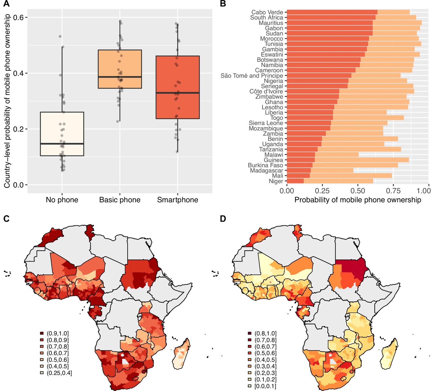
Basic mobile phone and smartphone ownership in 33 African countries.
(A) Boxplots show the probabilities of not owning a mobile phone (cream), owning a basic mobile phone (BP; orange), or owning a smartphone (SP; red). Country-level probabilities (dots) are overlaid and jittered to reduce overlap. (B) Barplot shows the country-level probabilities of BP ownership (orange) and SP ownership (red) ordered by SP ownership. Geographic distribution showing probabilities of (C) BP ownership and (D) SP ownership in 33 Afrobarometer countries at the sub-national level.
Figure 1—figure supplement 1
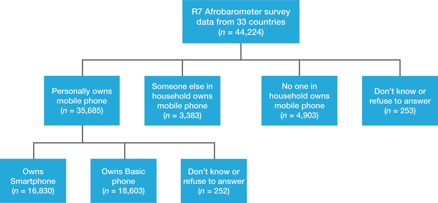
Flow diagram of participant sample sizes.
Shown for 33 countries that collect phone ownership data as part of the Afrobarometer Round 7 (R7) survey.
Figure 1—figure supplement 2
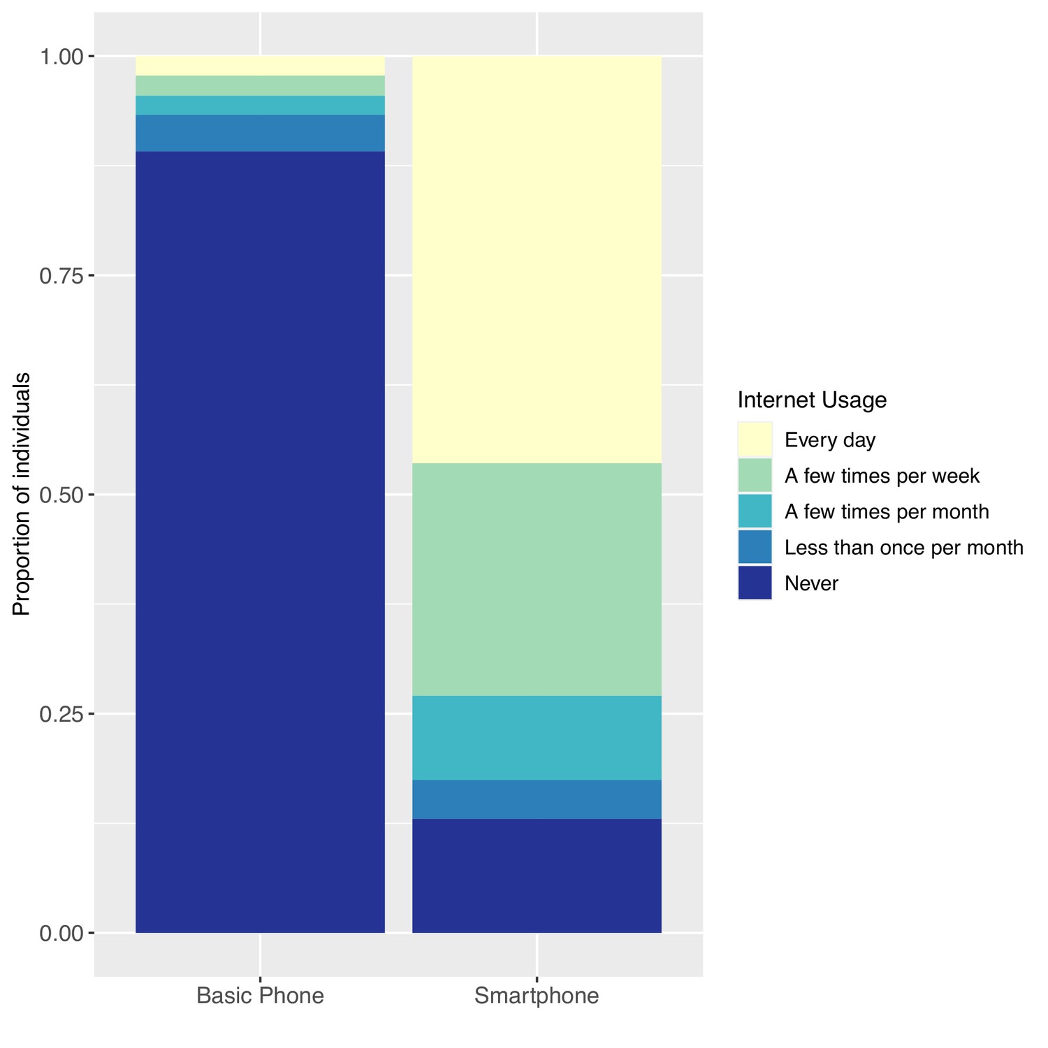
Internet usage by type of phone owned.
Afrobarometer Round 7 (R7) surveyed individuals on how often they used the internet. Individuals were not asked to specify how they used the internet (i.e. they did not necessarily have to use or own a phone to access the internet).
Figure 1—figure supplement 3
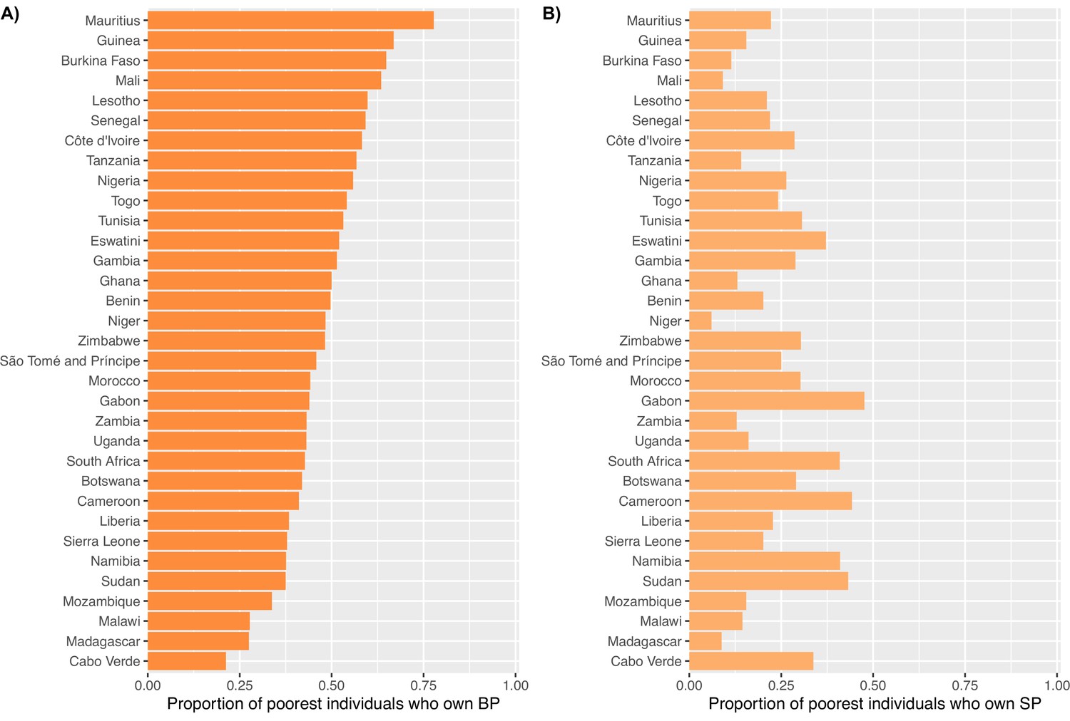
Phone ownership in the poorest individuals.
(A) Country-level basic mobile phone (BP) ownership in individuals with Lived Poverty Index (LPI) = 3. (B) Country-level smartphone (SP) ownership in individuals with LPI = 3.
Figure 2
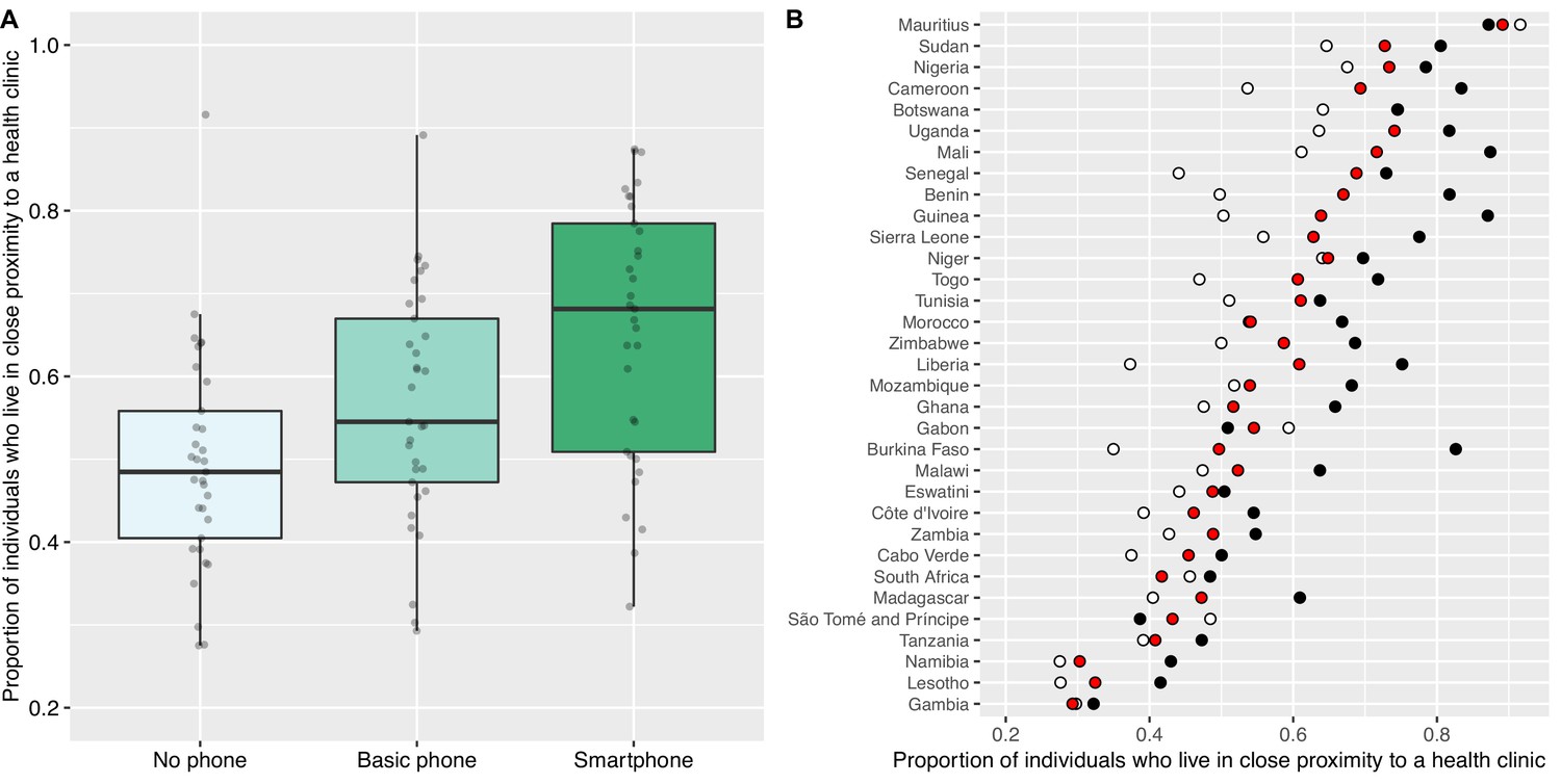
Proximity to health clinics and mobile phone ownership in 33 African countries.
(A) Boxplots show the proportion of individuals who live in close proximity to a health clinic (HC) based on whether they do not own a mobile phone (mean 0.49), own a basic mobile phone (BP; mean 0.56), or own a smartphone (SP; mean 0.66). Country-level probabilities (dots) are overlaid and jittered to reduce overlap. (B) Scatterplot shows the country-specific proportions of individuals who live in close proximity to an HC amongst individuals who: do not own a mobile phone (white dots), own a BP (red dots), or own an SP (black dots).
Figure 3
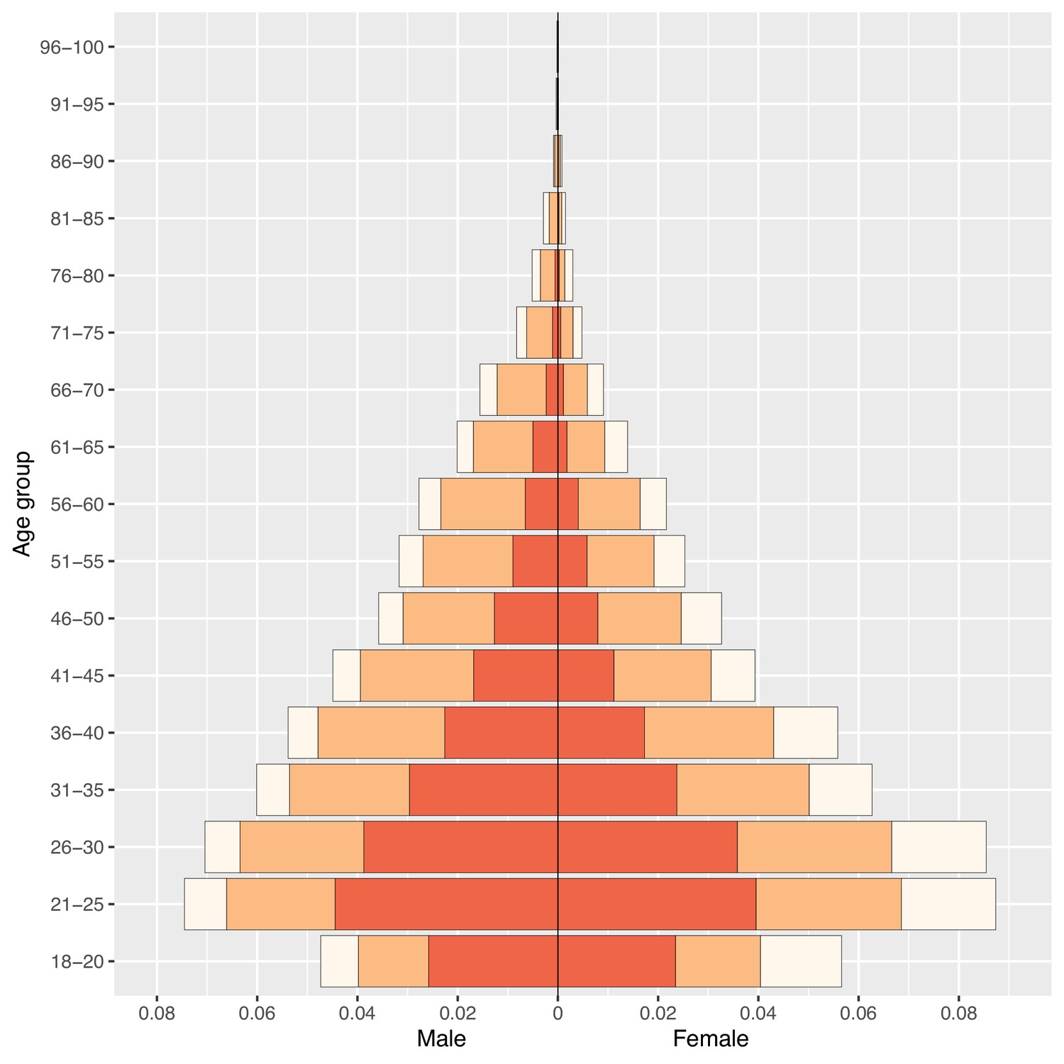
Phone ownership by age and gender in 33 African countries.
Population pyramid displays the distribution of the population stratified by gender and 5 year age groupings (with the exception of the 18–20 age class) by ownership of a mobile phone: no mobile phone (cream), a basic mobile phone (BP; orange), or a smartphone (SP; red).
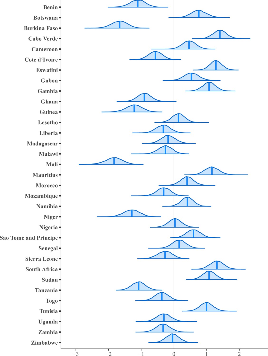
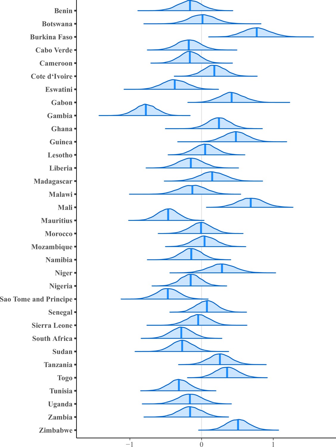
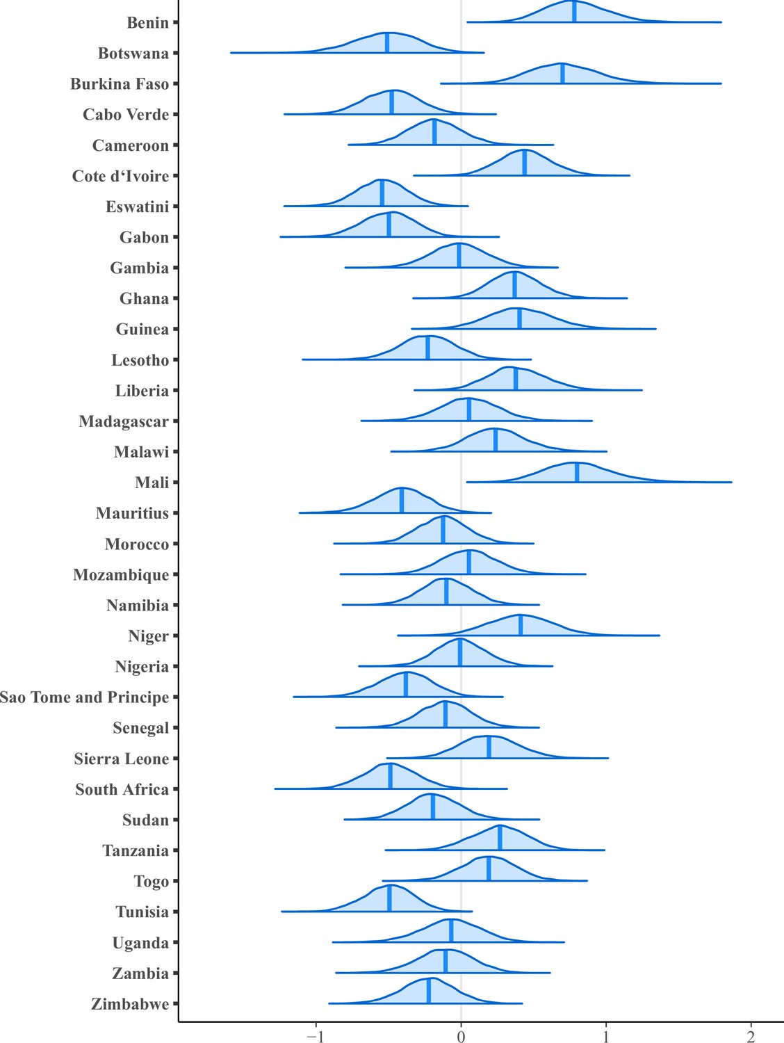
Figure 4 with 8 supplements
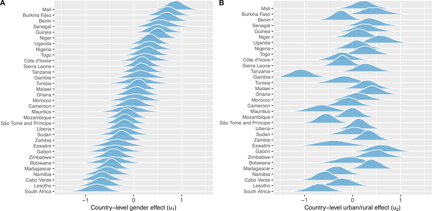
Country-level gender and urban-rural effects.
(A) Posterior distributions of the country-level effect on mobile phone ownership of being male (compared to female), sorted by median. (B) Posterior distributions of the country-level effect of living in an urban area (compared to living in a rural area), in the same country order as (A). Both (A) and (B) are on the logit-scale – and should be viewed respectively as country-specific adjustments to the population-level effect of (A) being male or (B) living in an urban area.
Figure 4—figure supplement 1
Model 1 posteriors – (country-level) intercept.
Posterior distributions (medians and 95% highest posterior density [HPD] regions) of , the country-level intercept, for country j.
Figure 4—figure supplement 2
Model 2 posteriors – (country-level) intercept.
Posterior distributions (medians and 95% highest posterior density [HPD] regions) of , the country-level intercept, for country j.
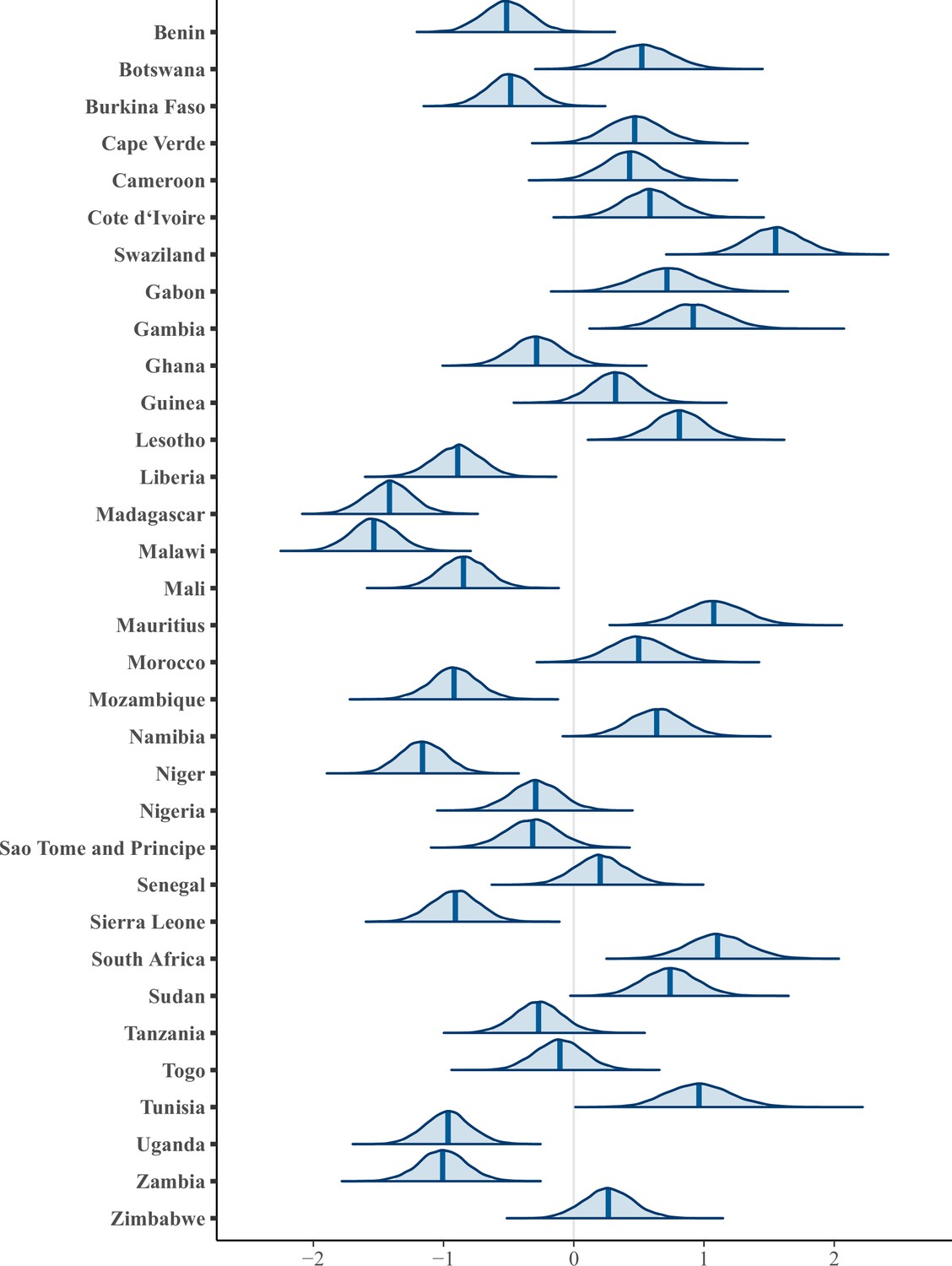
Figure 4—figure supplement 3
Model 2 posteriors – (country-level) urban/rural.
Posterior distributions (medians and 95% highest posterior density [HPD] regions) of , the country-level effect of living in an urban area, for country j.
Figure 4—figure supplement 4
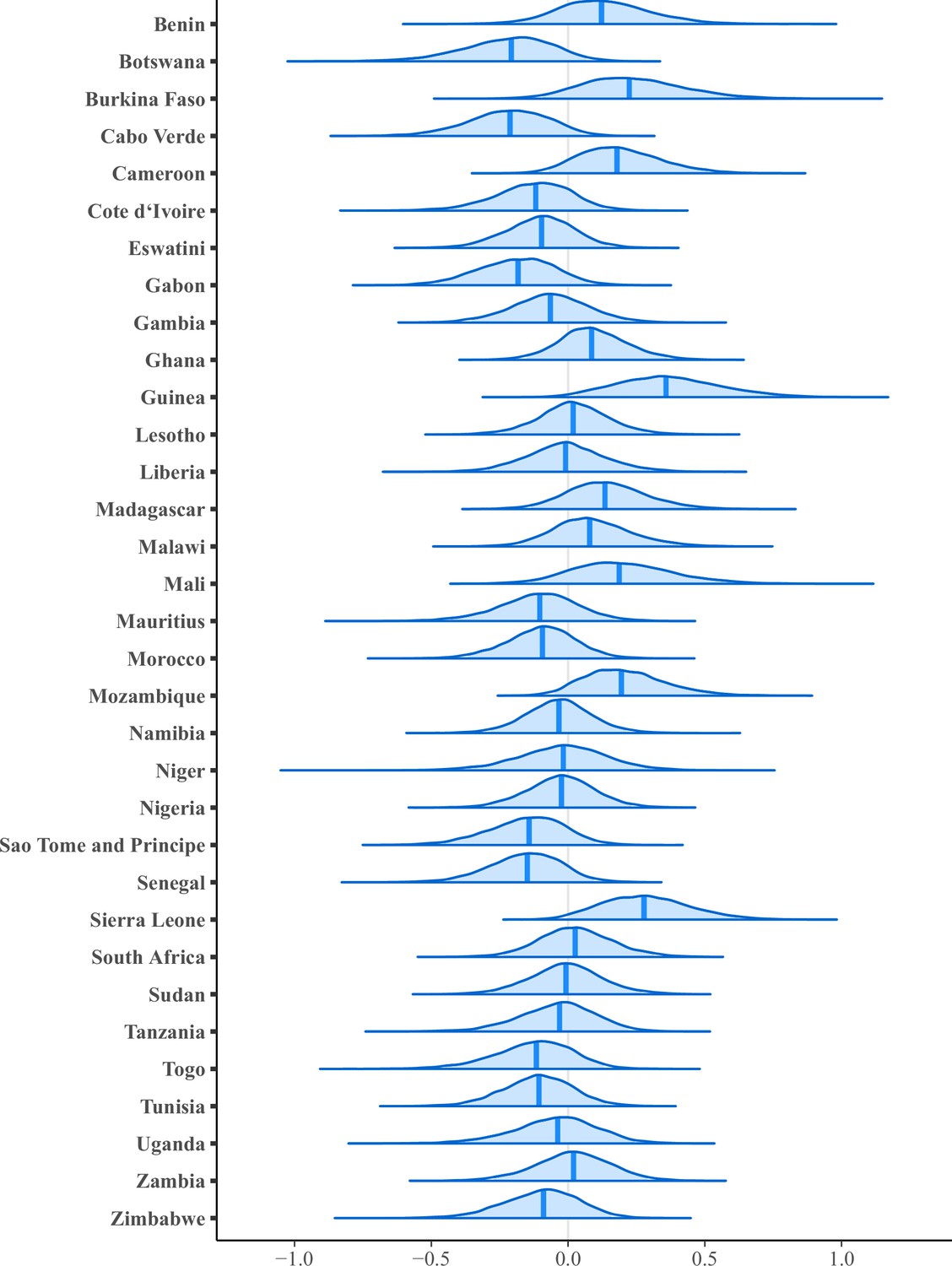
Model 2 posteriors – (country-level) gender and proximity I.
Posterior distributions (medians and 95% highest posterior density [HPD] regions) of , the country-level effect of being female in close proximity to a health clinic (HC), for country j.
Figure 4—figure supplement 5
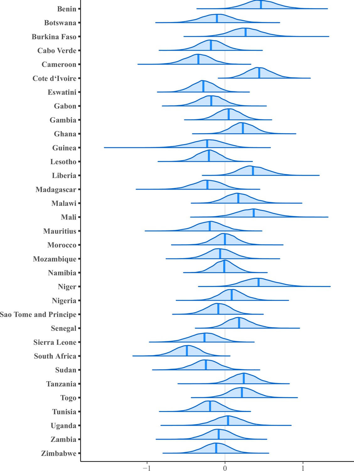
Model 2 posteriors – (country-level) gender and proximity II.
Posterior distributions (medians and 95% highest posterior density [HPD] regions) of , the country-level effect of being male not in close proximity to a health clinic (HC), for country j.
Figure 4—figure supplement 6
Model 2 posteriors – (country-level) gender and proximity III.
Posterior distributions (medians and 95% highest posterior density [HPD] regions) of , the country-level effect of being male in close proximity to a health clinic (HC), for country j.
Figure 4—figure supplement 7
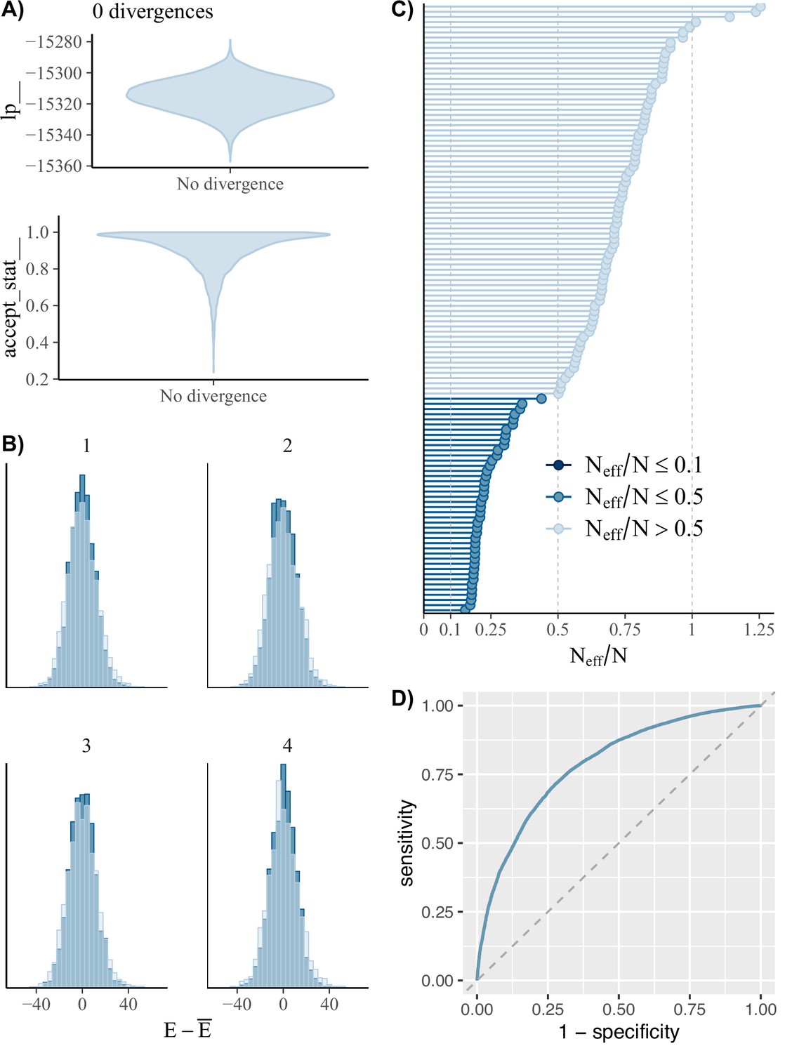
Model 1 Markov Chain Monte Carlo (MCMC) diagnostics and ROC curve.
(A) Violin plots of the log posterior (top) and No-U-Turn Sampling (NUTS) acceptance statistic (bottom). There are no divergent transitions. To further assess chain convergence, we used , the potential scale reduction factor (Gelman and Rubin, 1992). All values of are nearly equal to 1 , indicating all chains have converged. (B) NUTS energy plot (Betancourt, 2017) for all four chains. The transition distribution (darker histogram in each plot) and target distribution (lighter histogram in each plot) are moderately well aligned, indicating efficient sampling. (C) The effective sample size from the posterior distribution of each parameter was used to gauge the level of autocorrelation in each sample. for all model parameters indicating independent draws within each sample. (D) ROC curve used to assess the diagnostic capability of fitted Bayesian multilevel logistic regression (BMLR) model. The AUC was 0.79 indicating good predictive accuracy.
Figure 4—figure supplement 8

Model 2 Markov Chain Monte Carlo (MCMC) diagnostics and ROC curve.
(A) Violin plots of the log posterior (top) and No-U-Turn Sampling (NUTS) acceptance statistic (bottom). There are no divergent transitions. Additionally, all values of are nearly equal to 1 , indicating all chains have converged. (B) NUTS energy plot for all four chains. The transition distribution (darker histogram in each plot) and target distribution (lighter histogram in each plot) are moderately well aligned, indicating efficient sampling. (C) for all model parameters indicating independent draws within each sample. (D) ROC curve used to assess the diagnostic capability of fitted Bayesian multilevel logistic regression (BMLR) model. The AUC was 0.78 indicating good predictive accuracy.
Tables
Table 1
Probability of mobile phone ownership by country and gender.
| Country | Any mobile phone | Smartphone | |||||
|---|---|---|---|---|---|---|---|
| Female | Male | OR† | Female | Male | OR† | ||
| Benin | 0.66 | 0.90 | 4.78* | 0.19 | 0.41 | 2.84* | |
| Mali | 0.60 | 0.88 | 4.77* | 0.15 | 0.26 | 1.93* | |
| Burkina Faso | 0.67 | 0.90 | 4.31* | 0.18 | 0.27 | 1.64* | |
| Senegal | 0.83 | 0.95 | 3.90* | 0.44 | 0.52 | 1.40* | |
| Guinea | 0.79 | 0.93 | 3.46* | 0.22 | 0.23 | 1.06 | |
| Niger | 0.47 | 0.74 | 3.23* | 0.14 | 0.23 | 1.92* | |
| Cote d`Ivoire | 0.85 | 0.95 | 3.10* | 0.32 | 0.49 | 1.98* | |
| Nigeria | 0.78 | 0.91 | 3.02* | 0.48 | 0.54 | 1.29* | |
| Gambia | 0.85 | 0.94 | 2.82* | 0.60 | 0.65 | 1.23 | |
| Togo | 0.75 | 0.89 | 2.80* | 0.33 | 0.45 | 1.61* | |
| Uganda | 0.59 | 0.80 | 2.76* | 0.33 | 0.37 | 1.18 | |
| Tunisia | 0.92 | 0.97 | 2.45* | 0.61 | 0.60 | 0.97 | |
| Sierra Leone | 0.62 | 0.80 | 2.42* | 0.44 | 0.44 | 1.01 | |
| Tanzania | 0.74 | 0.87 | 2.41* | 0.23 | 0.31 | 1.50* | |
| Malawi | 0.41 | 0.61 | 2.29* | 0.34 | 0.43 | 1.49* | |
| Morocco | 0.90 | 0.95 | 2.28* | 0.60 | 0.64 | 1.22 | |
| Ghana | 0.82 | 0.91 | 2.15* | 0.35 | 0.47 | 1.70* | |
| Mauritius | 0.93 | 0.97 | 2.11* | 0.63 | 0.64 | 1.02 | |
| Cameroon | 0.85 | 0.92 | 2.10* | 0.55 | 0.54 | 0.96 | |
| Mozambique | 0.61 | 0.75 | 1.87* | 0.45 | 0.45 | 1.02 | |
| Sao Tome and Principe | 0.75 | 0.85 | 1.83* | 0.55 | 0.58 | 1.14 | |
| Liberia | 0.64 | 0.76 | 1.79* | 0.38 | 0.53 | 1.90* | |
| Sudan | 0.89 | 0.94 | 1.77* | 0.65 | 0.67 | 1.11 | |
| Eswatini | 0.92 | 0.95 | 1.74* | 0.57 | 0.60 | 1.14 | |
| Zambia | 0.63 | 0.73 | 1.61* | 0.40 | 0.41 | 1.06 | |
| Zimbabwe | 0.82 | 0.87 | 1.46* | 0.42 | 0.45 | 1.15 | |
| Madagascar | 0.44 | 0.50 | 1.29* | 0.36 | 0.36 | 1.00 | |
| Gabon | 0.93 | 0.94 | 1.26 | 0.63 | 0.66 | 1.13 | |
| Namibia | 0.88 | 0.90 | 1.24 | 0.54 | 0.62 | 1.40* | |
| Botswana | 0.89 | 0.91 | 1.23 | 0.55 | 0.62 | 1.33* | |
| Cabo Verde | 0.85 | 0.88 | 1.20 | 0.71 | 0.77 | 1.36* | |
| Lesotho | 0.84 | 0.86 | 1.18 | 0.39 | 0.39 | 1.02 | |
| South Africa | 0.91 | 0.91 | 0.97 | 0.69 | 0.68 | 0.93 | |
-
*
Significant at α=0.05.
-
†
Odds ratio of male phone ownership to female phone ownership.
Table 2
Probability of mobile phone ownership by country and urban/rural status.
| Country | Any mobile phone | Smartphone | |||||
|---|---|---|---|---|---|---|---|
| Rural | Urban | OR† | Rural | Urban | OR† | ||
| Gabon | 0.82 | 0.97 | 7.17* | 0.31 | 0.72 | 5.66* | |
| Zimbabwe | 0.78 | 0.95 | 5.94* | 0.28 | 0.64 | 4.58* | |
| Uganda | 0.63 | 0.90 | 5.58* | 0.29 | 0.49 | 2.42* | |
| Burkina Faso | 0.74 | 0.94 | 5.25* | 0.12 | 0.52 | 7.57* | |
| Ghana | 0.77 | 0.94 | 5.09* | 0.24 | 0.53 | 3.60* | |
| Senegal | 0.82 | 0.96 | 4.78* | 0.34 | 0.60 | 2.90* | |
| Morocco | 0.86 | 0.97 | 4.70* | 0.42 | 0.71 | 3.51* | |
| Zambia | 0.56 | 0.84 | 4.23* | 0.29 | 0.50 | 2.54* | |
| Madagascar | 0.40 | 0.73 | 4.17* | 0.27 | 0.54 | 3.25* | |
| Togo | 0.76 | 0.93 | 4.14* | 0.25 | 0.57 | 3.92* | |
| Tanzania | 0.75 | 0.92 | 4.00* | 0.17 | 0.42 | 3.45* | |
| Malawi | 0.45 | 0.76 | 3.87* | 0.33 | 0.54 | 2.37* | |
| Guinea | 0.82 | 0.95 | 3.84* | 0.12 | 0.42 | 5.11* | |
| Liberia | 0.58 | 0.84 | 3.69* | 0.35 | 0.55 | 2.33* | |
| Botswana | 0.84 | 0.95 | 3.65* | 0.43 | 0.73 | 3.56* | |
| Mali | 0.70 | 0.88 | 3.24* | 0.13 | 0.47 | 6.09* | |
| Niger | 0.57 | 0.80 | 3.10* | 0.14 | 0.37 | 3.63* | |
| Sudan | 0.89 | 0.96 | 3.09* | 0.59 | 0.76 | 2.16* | |
| Nigeria | 0.79 | 0.92 | 3.05* | 0.42 | 0.61 | 2.20* | |
| Lesotho | 0.82 | 0.93 | 2.91* | 0.27 | 0.57 | 3.62* | |
| Mozambique | 0.60 | 0.81 | 2.86* | 0.33 | 0.60 | 3.02* | |
| Cameroon | 0.83 | 0.93 | 2.74* | 0.43 | 0.64 | 2.42* | |
| Cote d`Ivoire | 0.86 | 0.94 | 2.45* | 0.26 | 0.55 | 3.35* | |
| Tunisia | 0.91 | 0.96 | 2.32* | 0.52 | 0.64 | 1.62* | |
| Sierra Leone | 0.64 | 0.80 | 2.28* | 0.32 | 0.55 | 2.61* | |
| Namibia | 0.85 | 0.93 | 2.22* | 0.44 | 0.68 | 2.72* | |
| Benin | 0.72 | 0.85 | 2.18* | 0.23 | 0.40 | 2.21* | |
| Eswatini | 0.93 | 0.97 | 2.17 | 0.56 | 0.73 | 2.17* | |
| Cabo Verde | 0.82 | 0.89 | 1.69* | 0.63 | 0.79 | 2.26* | |
| South Africa | 0.89 | 0.92 | 1.36 | 0.57 | 0.74 | 2.07* | |
| Sao Tome and Principe | 0.77 | 0.82 | 1.34* | 0.52 | 0.59 | 1.30 | |
| Mauritius | 0.95 | 0.95 | 0.98 | 0.61 | 0.67 | 1.29* | |
| Gambia | 0.92 | 0.89 | 0.71 | 0.61 | 0.64 | 1.15 | |
-
*
Significant at α=0.05.
-
†
Odds ratio of urban phone ownership to rural phone ownership.
Table 3
Fitted Bayesian models for determinants of mobile phone ownership in Africa.
| Population-level effects | Bivariable (Bayesian logistic regression [BLR] models) | Multivariable (Bayesian multilevel logistic regression [BMLR] model 1) | ||
|---|---|---|---|---|
| Crude OR | 95% highest posterior density (HPD) region† | aOR | 95% highest posterior density (HPD) region† | |
| Female | ref | - | ref | - |
| Male | 2.04 | (1.94, 2.16)* | 2.37 | (1.96, 2.84)* |
| Rural | ref | - | ref | - |
| Urban | 3.47 | (3.27, 3.68)* | 2.66 | (2.22, 3.18)* |
| Age (61+) | ref | - | ref | - |
| 18–20 | 1.36 | (1.21, 1.53)* | 1.73 | (1.51, 1.96)* |
| 21–25 | 1.75 | (1.59, 1.93)* | 2.29 | (2.05, 2.56)* |
| 26–40 | 1.98 | (1.82, 2.15)* | 2.68 | (2.44, 2.94)* |
| 41–50 | 1.85 | (1.68, 2.03)* | 2.44 | (2.19, 2.72)* |
| 51–60 | 1.54 | (1.39, 1.71)* | 1.78 | (1.59, 2.00)* |
| Lived Poverty Index (LPI) = 0 (wealthiest) | ref | - | ref | - |
| LPI = 1 | 0.50 | (0.44, 0.56)* | 0.69 | (0.61, 0.78)* |
| LPI = 2 | 0.29 | (0.26, 0.32)* | 0.46 | (0.41, 0.52)* |
| LPI = 3 (poorest) | 0.24 | (0.21, 0.26)* | 0.35 | (0.31, 0.40)* |
| No health clinic (HC) in close proximity | ref | - | ref | - |
| HC in close proximity | 1.56 | (1.49, 1.65)* | 1.31 | (1.24, 1.39)* |
| Country-level effects | Estimate | 95% highest posterior density (HPD) region† | ||
| 0.87 | (0.67, 1.11) | |||
| 0.48 | (0.33, 0.62) | |||
| 0.49 | (0.36, 0.64) | |||
| –0.43 | (–0.73, –0.13) | |||
| –0.32 | (–0.63, –0.02) | |||
| 0.21 | (–0.16, 0.55) | |||
-
*
Significant at α=0.05.
-
†
Bayesian 95% HPD regions.
Table 4
Fitted Bayesian models for determinants of smartphone ownership among mobile phone owners in Africa.
| Population-level effects | Bivariable (Bayesian logistic regression [BLR] models) | Multivariable (Bayesian multilevel logistic regression [BMLR] model 2) | ||
|---|---|---|---|---|
| Crude OR | 95% highest posterior density (HPD) region† | aOR | 95% highest posterior density (HPD) region† | |
| Female, no health clinic (HC) in close proximity | ref | - | ref | - |
| Female, HC in close proximity | 1.23 | (1.15, 1.32)* | 1.15 | (1.03, 1.30)* |
| Male, no HC in close proximity | 1.10 | (1.03, 1.18)* | 1.50 | (1.30, 1.72)* |
| Male, HC in close proximity | 1.54 | (1.44, 1.65)* | 1.92 | (1.63, 2.26)* |
| Rural | ref | - | ref | - |
| Urban | 2.95 | (2.81, 3.09)* | 2.67 | (2.33, 3.10)* |
| Age (61+) | ref | - | ref | - |
| 18–30 | 5.59 | (5.08, 6.16)* | 7.85 | (7.04, 8.77)* |
| 31–40 | 3.53 | (3.19, 3.90)* | 4.73 | (4.24, 5.30)* |
| 41–50 | 2.25 | (2.02, 2.50)* | 2.75 | (2.44, 3.09)* |
| 51–60 | 1.58 | (1.41, 1.77)* | 1.72 | (1.51, 1.96)* |
| Lived Poverty Index (LPI) = 0 (wealthiest) | ref | - | ref | - |
| LPI = 1 | 0.61 | (0.57, 0.66)* | 0.67 | (0.62, 0.73)* |
| LPI = 2 | 0.38 | (0.35, 0.40)* | 0.45 | (0.41, 0.49)* |
| LPI = 3 (poorest) | 0.27 | (0.25, 0.29)* | 0.35 | (0.32, 0.39)* |
| Country-level effects | Estimate | 95% highest posterior density (HPD) region† | ||
| 0.85 | (0.67, 1.05) | |||
| 0.39 | (0.28, 0.50) | |||
| 0.21 | (0.08, 0.34) | |||
| 0.31 | (0.18, 0.43) | |||
| 0.41 | (0.28, 0.53) | |||
| –0.61 | (–0.81, –0.37) | |||
| –0.38 | (–0.77, 0.01) | |||
| –0.51 | (–0.80, –0.19) | |||
| –0.78 | (–0.93, –0.60) | |||
| 0.10 | (–0.38, 0.54) | |||
| 0.16 | (–0.24, 0.55) | |||
| 0.29 | (–0.06, 0.60) | |||
| –0.07 | (–0.59, 0.41) | |||
| 0.47 | (0.04, 0.82) | |||
| 0.61 | (0.30, 0.88) | |||
-
*
Significant at α=0.05.
-
†
Bayesian 95% HPD regions.
Additional files
Download links
A two-part list of links to download the article, or parts of the article, in various formats.
Downloads (link to download the article as PDF)
Open citations (links to open the citations from this article in various online reference manager services)
Cite this article (links to download the citations from this article in formats compatible with various reference manager tools)
Lack of ownership of mobile phones could hinder the rollout of mHealth interventions in Africa
eLife 11:e79615.
https://doi.org/10.7554/eLife.79615


