Stable population structure in Europe since the Iron Age, despite high mobility
- Biomedical Informatics Program, Stanford University, United States
- Department of Genetics, Stanford University, United States
- Department of Genetics, University of Pennsylvania, Perelman School of Medicine, United States
- Department of Evolutionary Anthropology, University of Vienna, Austria
- Human Evolution and Archaeological Sciences, University of Vienna, Austria
- Stanford Archaeology Center, Stanford University, United States
- University of Chicago, Department of Human Genetics, United States
- Department of History and Art History, Utrecht University, Netherlands
- CIAS, Department of Life Sciences, University of Coimbra, Portugal
- Dipartimento di Storia Antropologia Religioni Arte Spettacolo, Sapienza University, Italy
- Archaeological Museum Zadar, Croatia
- LBEIG, Population Genetics & Conservation Unit, Department of Cellular and Molecular Biology – Faculty of Biological Sciences, University of Sciences and Technology Houari Boumediene, Algeria
- National Academy of Sciences of Armenia, Institute of Archaeology and Ethnography, Armenia
- French National Institute for Preventive Archaeological Research (INRAP)/CAGT UMR 5288, France
- Centre for Applied Bioanthropology, Institute for Anthropological Research, Croatia
- Université Gustave Eiffel – Laboratoire ACP, France
- Palisada Ltd, Croatia
- Dipartimento dei Beni Culturali, Archeologia, Storia dell'arte, del Cinema e della Musica, Università di Padova, Italy
- Department of Anthropology, Faculty of Biology and Environmental Protection, University of Lodz, Poland
- Aix Marseille Université, CNRS, Centre Camille Jullian, France
- Kaducej Ltd, Croatia
- Faculty of Humanities and Social Sciences, University of Zagreb, Croatia
- Bioarchaeology Service, Museum of Civilizations, Italy
- Museo Archeologico Nazionale di Tarquinia, Direzione Regionale Musei Lazio, Italy
- Archaeological Museum in Zagreb, Croatia
- Institute of Archaeology, Slovak Academy of Sciences, Slovakia
- Département des Monuments et des Sites Antiques - Institut National du Patrimoine INP, Tunisia
- University of Ljubljana, Faculty of Arts, Department for Archaeology, Slovenia
- Soprintendenza Archeologia, belle arti e paesaggio per le province di Sassari e Nuoro, Italy
- Department of Oriental Studies, Sapienza University of Rome, Italy
- Institute of Archaeology Belgrade, Serbia
- Institute of Biomedical Sciences, Vilnius University, Lithuania
- Institute of Archaeology, Croatia
- Université de Lorraine, Centre de Recherche Universitaire Lorrain d' Histoire (CRULH), France
- Department of Archaeologi, Shirak Centere of Armenological Studies, National Academy of Sciences Republic of Armenia, Armenia
- Institute of Archaeology and Ethnography of the National Academy of Sciences of the Republic of Armenia, Armenia
- Musée Archéologique de l'Oise, France
- Department of Environmental Biology, Sapienza University of Rome, Italy
- UMR 7041 ArScAn / French Institute of the Near East, Lebanon
- Archaeology Division, Croatian Academy of Sciences and Arts, Croatia
- CEF - University of Coimbra, Portugal
- UNIARQ - University of Lisbon, Portugal
- Skupina STIK Zavod za preučevanje povezovalnih področij preteklosti in sedanjosti, Slovenia
- Cardiolo-Oncology Research Collaborative Group (CORCG), Faculty of Medicine, Benyoucef Benkhedda University, Algeria
- Molecular Pathology, University Paul Sabatier Toulouse III, France
- French National Institute for Preventive Archaeological Research (INRAP), France
- Museum of Croatian Archaeological Monuments, Croatia
- L’Institut français du Proche-Orient, Lebanon
- Institute of Archaeology and Ethnology Polish Academy of Sciences, Centre of Interdisciplinary Archaeological Research, Poland
- Department of Odontostomatological and Maxillofacial Sciences, Sapienza University of Rome, Italy
- Austrian Archaeological Institute, Austrian Academy of Sciences, Austria
- Institute of Prehistory and Early History, University of Vienna, Austria
- Thuringia State Service for Cultural Heritage and Archaeology Weimar, Germany
- Institute of Anatomy and Cell Biology, University Medical Centre, Georg-August University of Göttingen, Germany
- Mississippi State University, United States
- University of Nevada, United States
- Trogir Town Museum, Croatia
- Université Paris 1 Panthéon-Sorbonne, France
- Faculty of Archaeology, University of Warsaw, Poland
- Dipartimento Asia, Africa e Mediterraneo, Università degli Studi di Napoli “L’Orientale”, Italy
- Museum of Vojvodina, Serbia
- Department of Anthropology, Natural History Museum Vienna, Austria
- Chair and Department of Normal Anatomy, Faculty of Medicine and Dentistry, Pomeranian Medical University, Poland
- Musée de La Cour d'Or, Eurométropole de Metz, France
- Department of Archeology, Center for Conservation and Archeology of Montenegro, Montenegro
- Insitut d’Archeologie, University Algiers 2, Algeria
- Université de Franche Comté / UMR Chrono-Environnement, France
- Anthropological Centre, Croatian Academy of Sciences and Arts, Croatia
- Department of Anthropology, New York University, United States
- Department of Genetics, Harvard Medical School, United States
- Department of Biology, Stanford University, United States
Figures
Figure 1 with 1 supplement
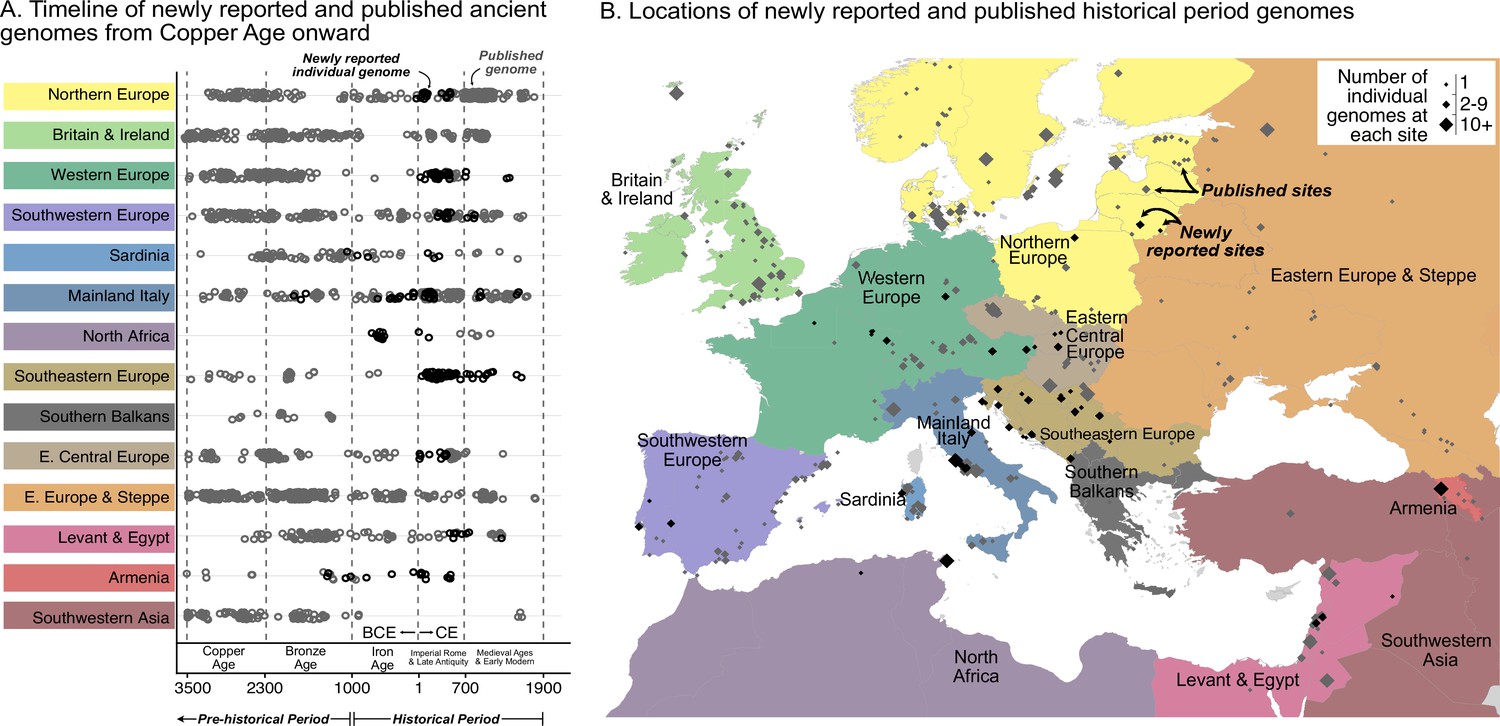
Timeline of new and published genomes.
(A) 204 newly reported genomes (black circles) are shown alongside published genomes (gray circles), ordered by time and region (colored the same way as in B). (B) Sampling locations of newly reported (black) and published (gray) genomes are indicated by diamonds, sized according to the number of genomes at each location.
Figure 1—figure supplement 1
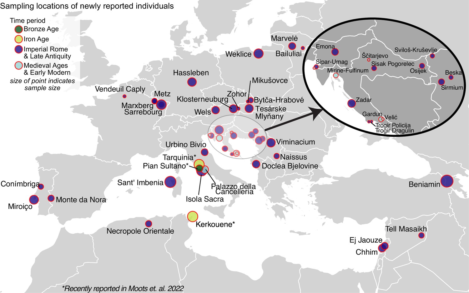
Detailed map of locations for newly reported samples.
Each circle represents a location, the size of the circle corresponds to the number of individuals sampled from that location. Circles are colored by their time period: Bronze Age is green (Pian Sultano), Iron Age is yellow (two recently reported sites Tarquinia and Kerkouane), Imperial Rome and Late Antiquity is dark blue, Medieval Ages and Early Modern are light blue (Palazzo della Cancelleria, Velić, Gardun, Mirine-Fulfinum). Note that the Bronze Age and Iron Age sites were recently reported in Moots et al., 2022.
Figure 2 with 3 supplements
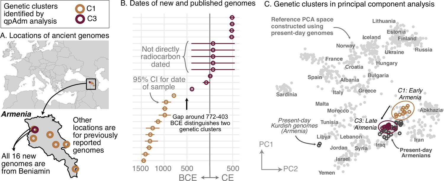
Armenia: two homogeneous genetic clusters distinguished by a temporal shift.
(A) Sampling locations of ancient genomes (open circles) colored by their genetic cluster identified using qpAdm modeling. (B) Date ranges for the genomes: each line represents the 95% confidence interval for the radiocarbon date or the upper and lower limit of the inferred date, and the point represents the midpoint of that range. (C) Projections of the genomes onto a PCA of present-day genomes (gray points labeled by their population). Present-day genomes from Armenia are shown with dark gray open circles.
Figure 2—figure supplement 1
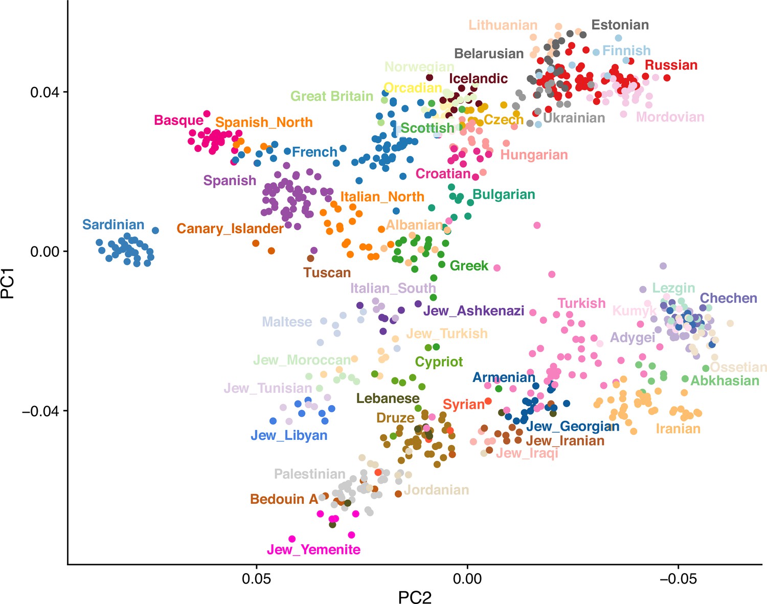
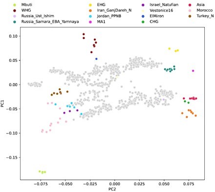
Principal component analysis of present-day genomes from Europe and the Mediterranean.
PCA was performed on 829 individuals (480,712 snps) using smartpca v1600. The following parameters were used: 5 outlier iterations (numoutlieriter), 10 principal components along which to remove outliers (numoutlierevec), altnormstyle set to NO, with least squares projection turned on (lsqproject set to YES).
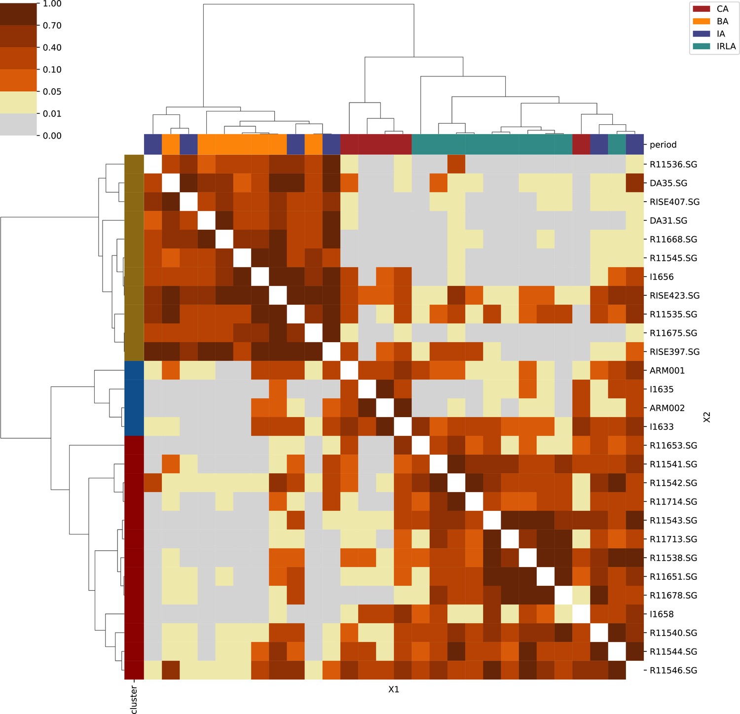
Figure 2—figure supplement 2
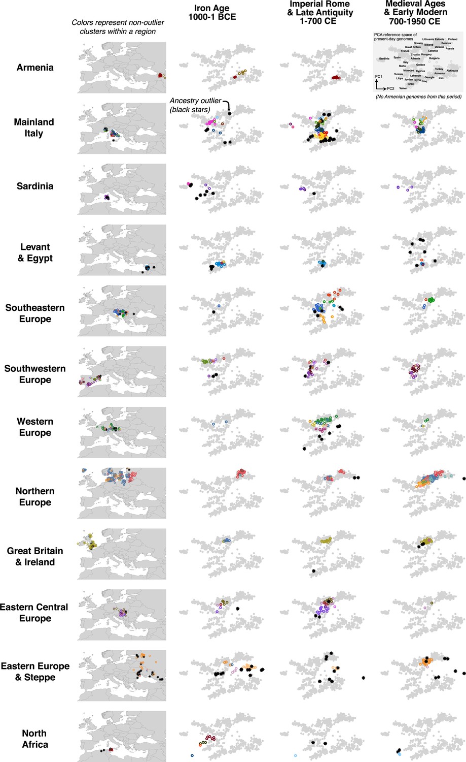
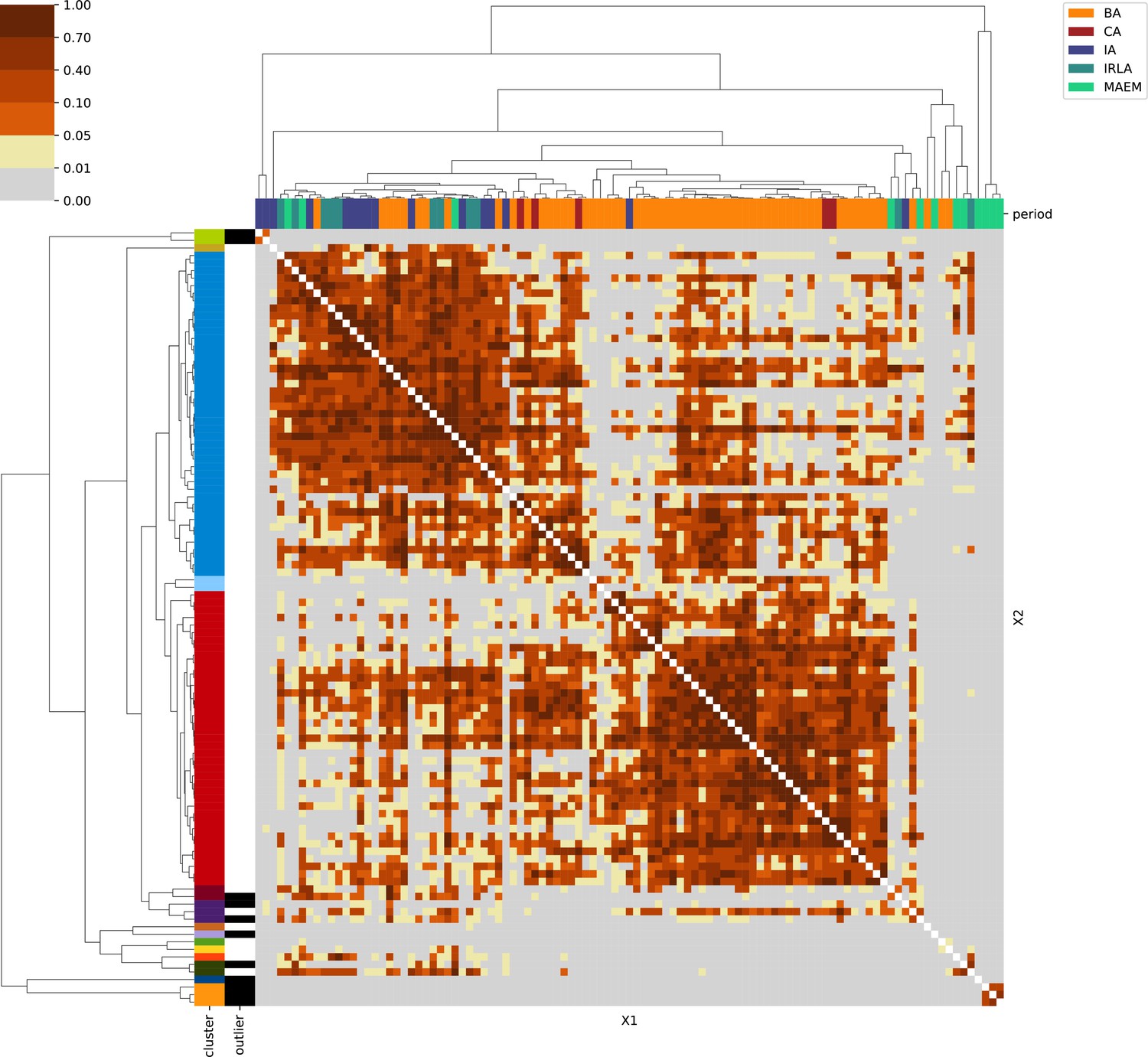
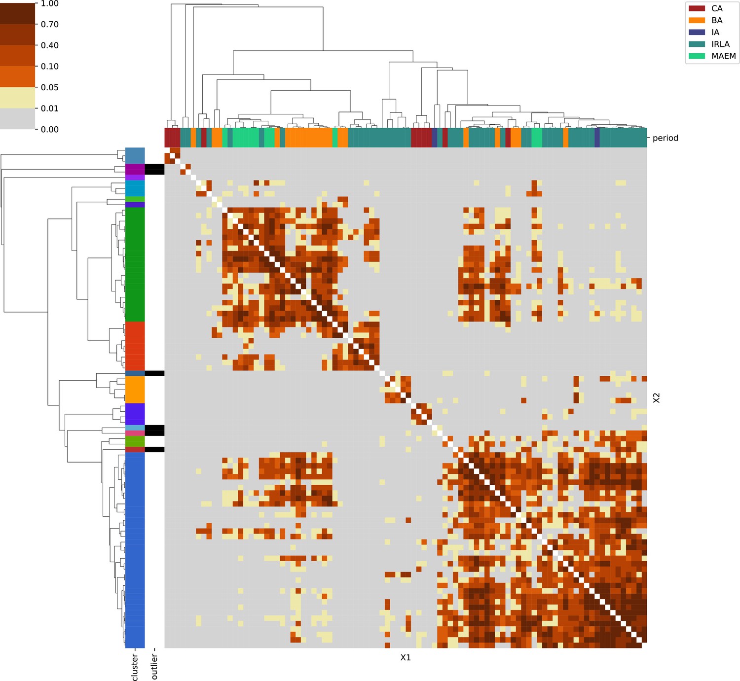
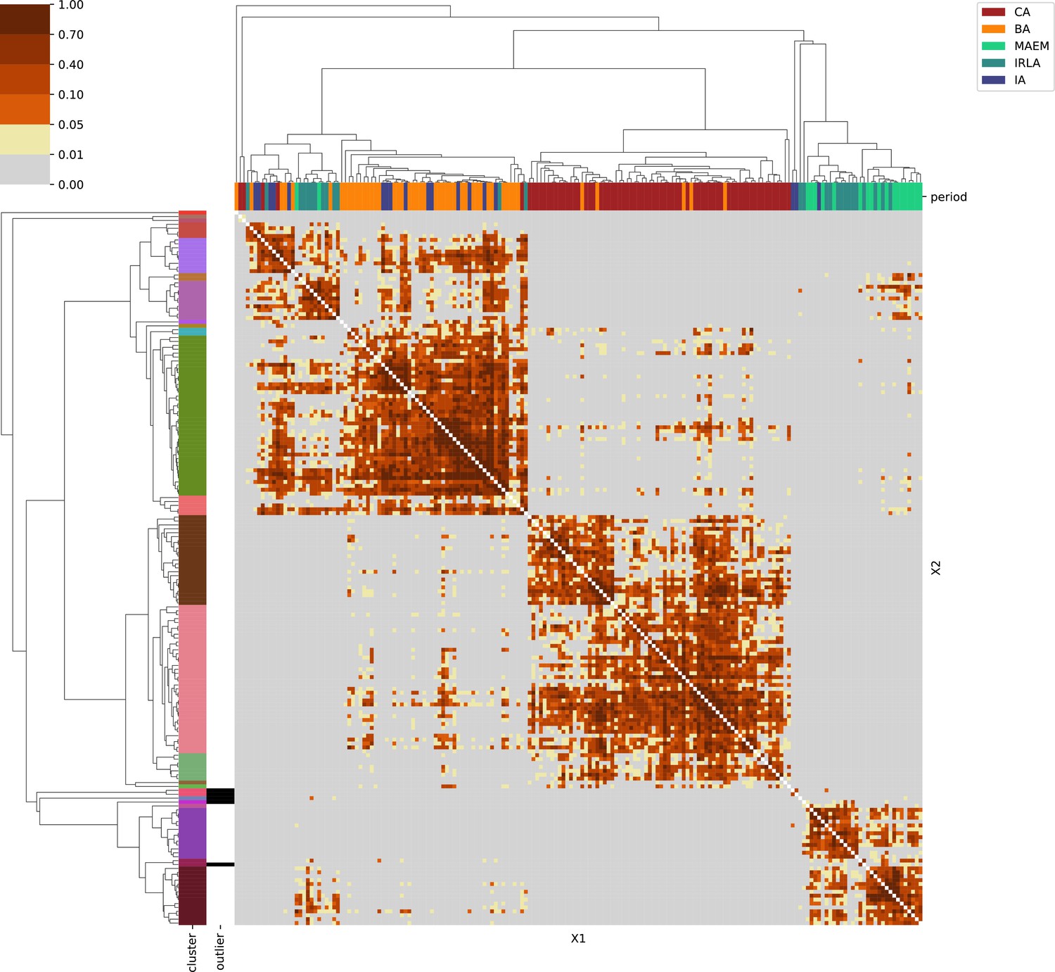
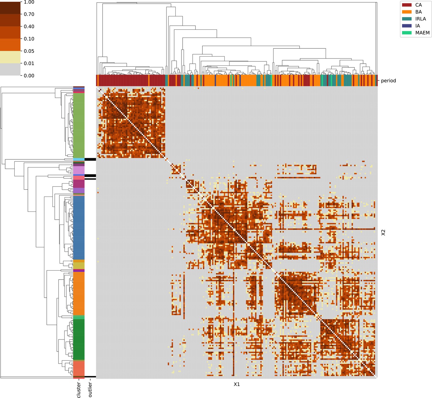
Ancestry clusters identified within regions.
Each row displays data from a single study region. The first column shows a map with the sampling locations for the individuals, while columns two through four show the individuals projected onto a PCA space of present-day genomes (gray points) (populations are labeled in the far right panel in row 1 and in Figure 2—figure supplement 1). Individual ancient genomes in the map and PCA panels are colored by ancestry clusters identified using qpAdm. Colors are not matched across regions. Star points are putative outliers, that is individuals with ancestry that is underrepresented in the region. They are not colored by ancestry clusters so as to reduce visual clutter.
Figure 2—figure supplement 3
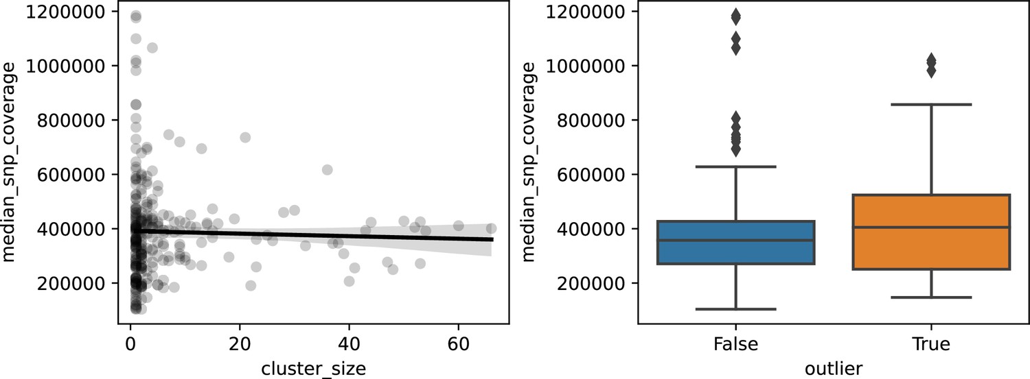
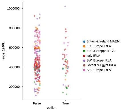
SNP coverage comparison across cluster sizes and downstream outlier status.
(left) No significant correlation was detected between the median number of SNPs covered across the individuals in a cluster and cluster size. (right) There also was no significant difference in the number of SNPs covered between outlier and non-outlier clusters.
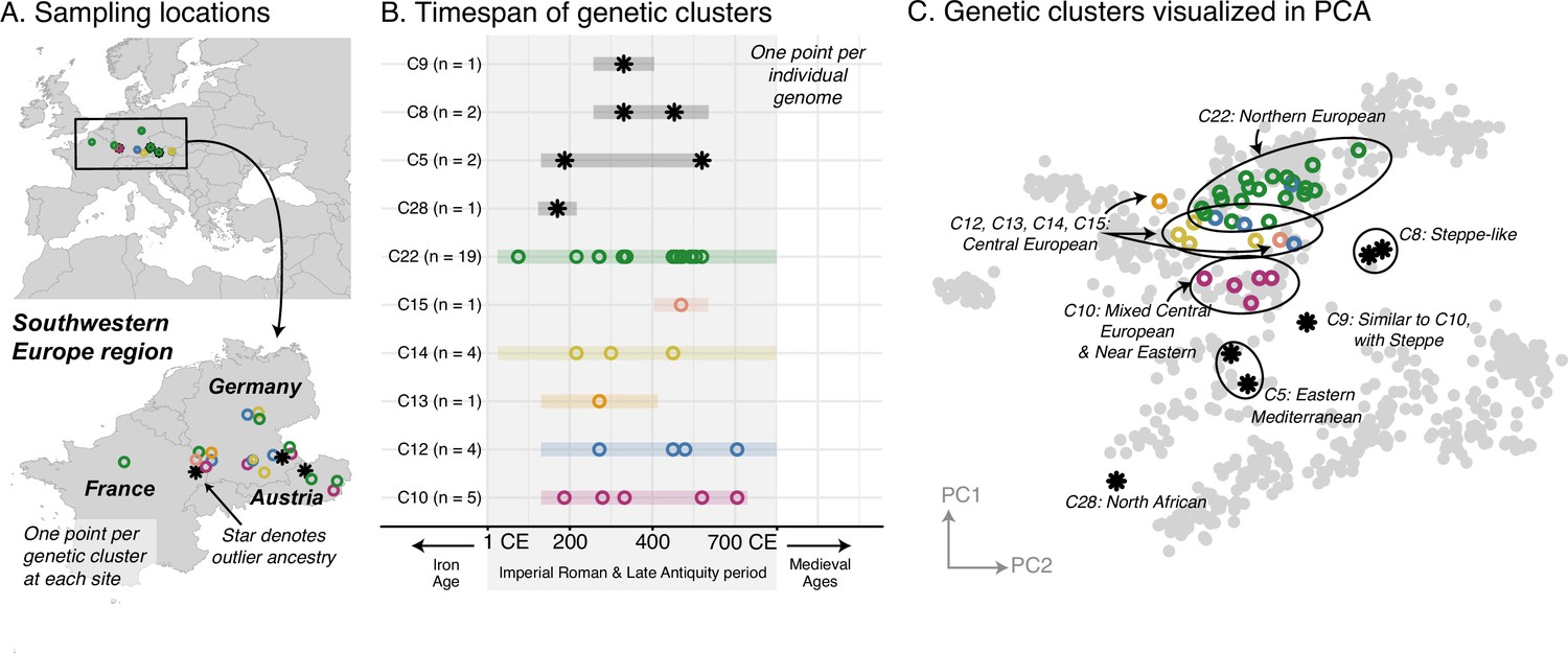
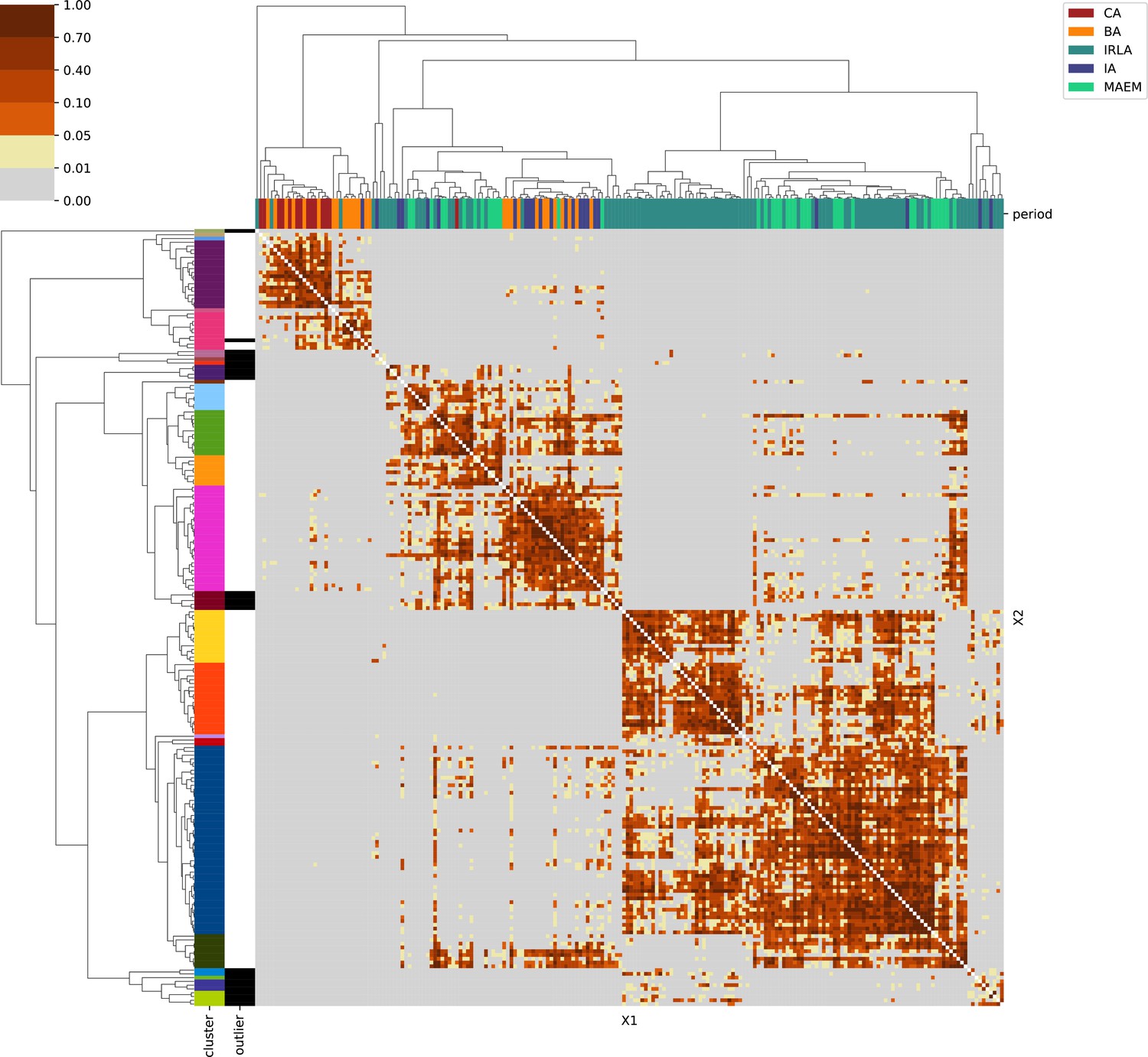
Figure 3 with 1 supplement
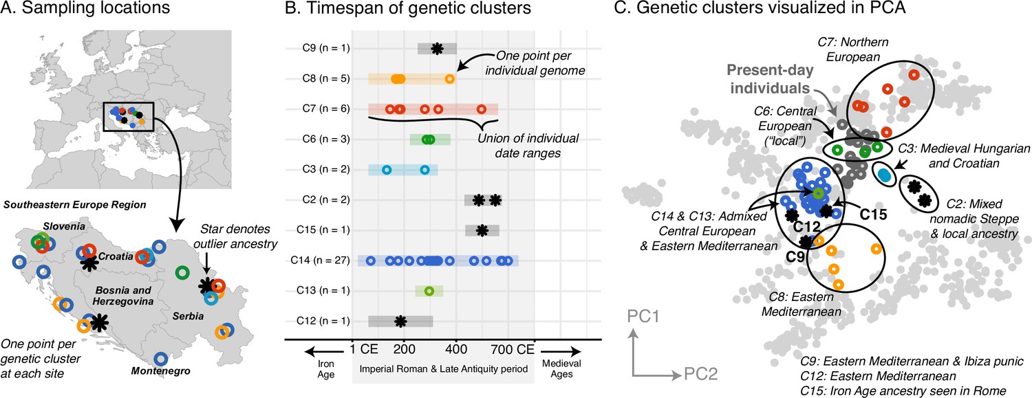
Southeastern Europe: highly heterogeneous Imperial Roman and Late Antiquity period population.
(A) Sampling locations of genetic clusters are represented by a single point per location. Outlier ancestries are black stars, all others are open circles colored by genetic cluster. (B) Colored bars span the minimum and maximum of the date ranges of samples (95% confidence interval from radiocarbon dating or archaeological range). Points are the mean of an individual’s date range. (C) Projections of the ancient genomes onto a PCA of present-day genomes (gray points). Population labels for the PCA reference space are shown in Figure 2C. Present-day genomes from Southeastern Europe are shown with dark gray open circles.
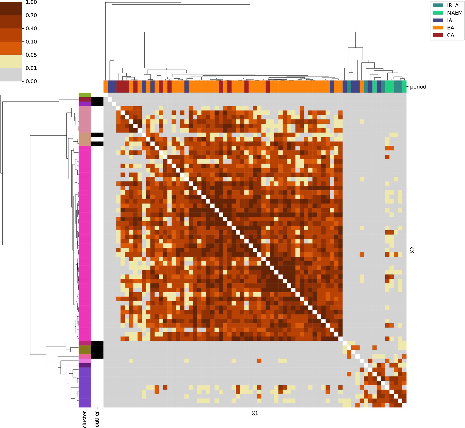
Figure 3—figure supplement 1
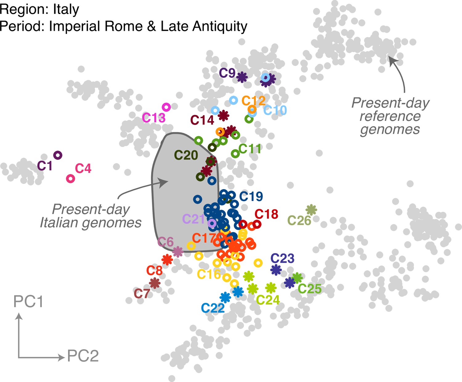
Population structure of Italy during the Imperial Roman and Late Antiquity period.
Ancient Italian genomes (colored points) from the Imperial Roman and Late Antiquity period were projected onto principal components of present-day genomes (gray points, populations labeled in Figure 2—figure supplement 1). Present-day Italian genomes are highlighted by a gray filled ellipse. Star points are outliers and circle points are non-outliers. Outlier clusters that can be modeled using contemporaneous populations are labeled with the potential source region.
Figure 4
Western Europe: heterogeneous Imperial Roman and Late Antiquity period population.
(A) Sampling locations of genetic clusters are represented by a single point per location. Outlier ancestries are black stars, all others are open circles colored by genetic cluster. (B) Colored bars span the minimum and maximum of the date ranges of samples (95% confidence interval from radiocarbon dating or archaeological range). Points are the mean of an individual’s date range. (C) Projections of the ancient genomes onto a PCA of present-day genomes (gray points). Population labels for the PCA reference space are shown in Figure 2C. Present-day genomes from Southeastern Europe are shown with dark gray open circles.
Figure 5 with 3 supplements
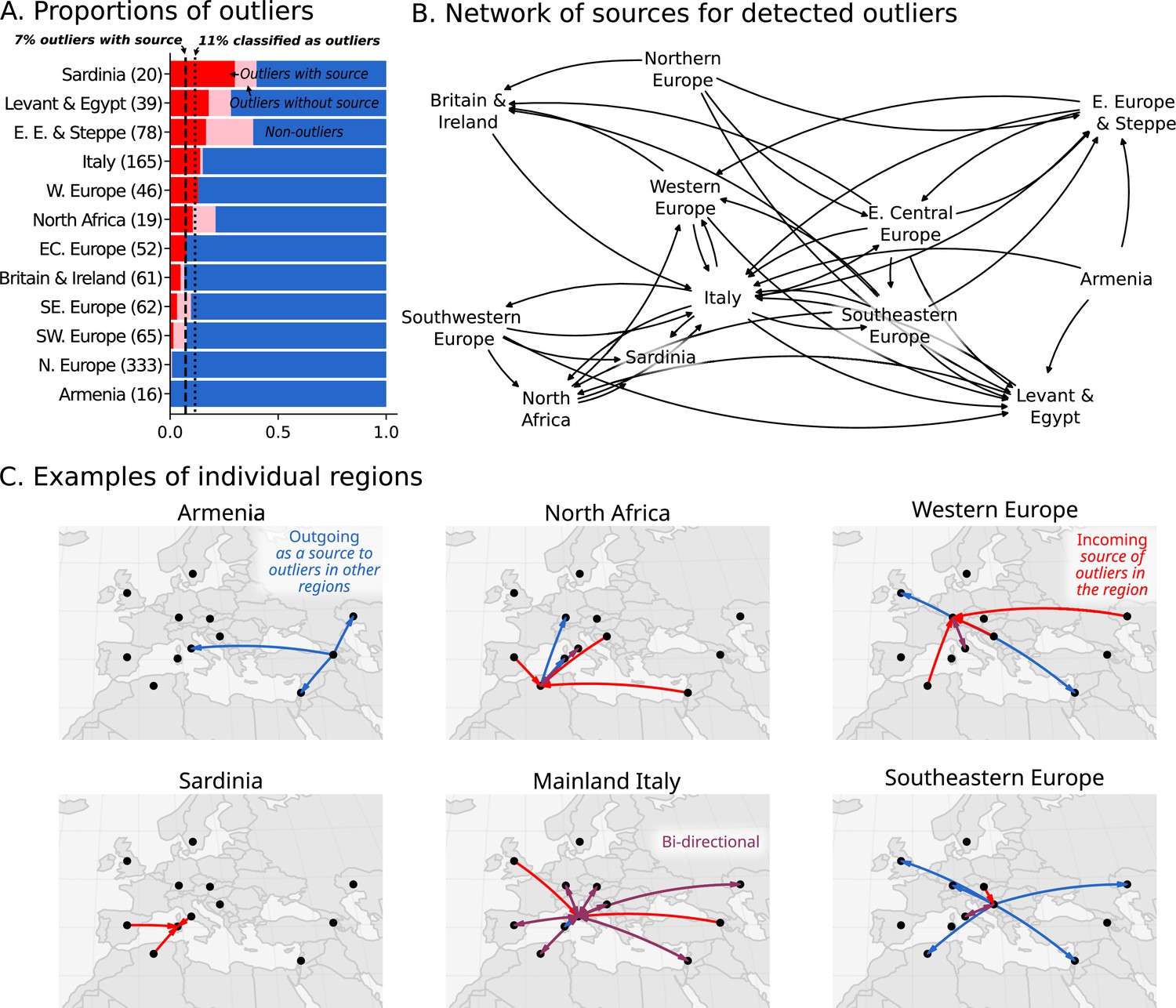
Ancestry outliers and their potential sources.
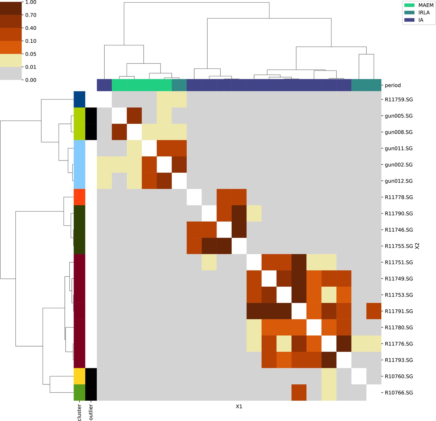
(A) The proportions of outliers in each region were determined by individual pairwise qpAdm modeling followed by clustering. (B) Sources were inferred by one component qpAdm modeling of resulting clusters with all genetic clusters in the dataset. In the network visualizations, nodes are regions and directed edges are drawn from sources to outliers (i.e. potential migrants). The full network of source to outlier is shown. (C) Examples of individual regions are shown in greater detail.
Figure 5—figure supplement 1
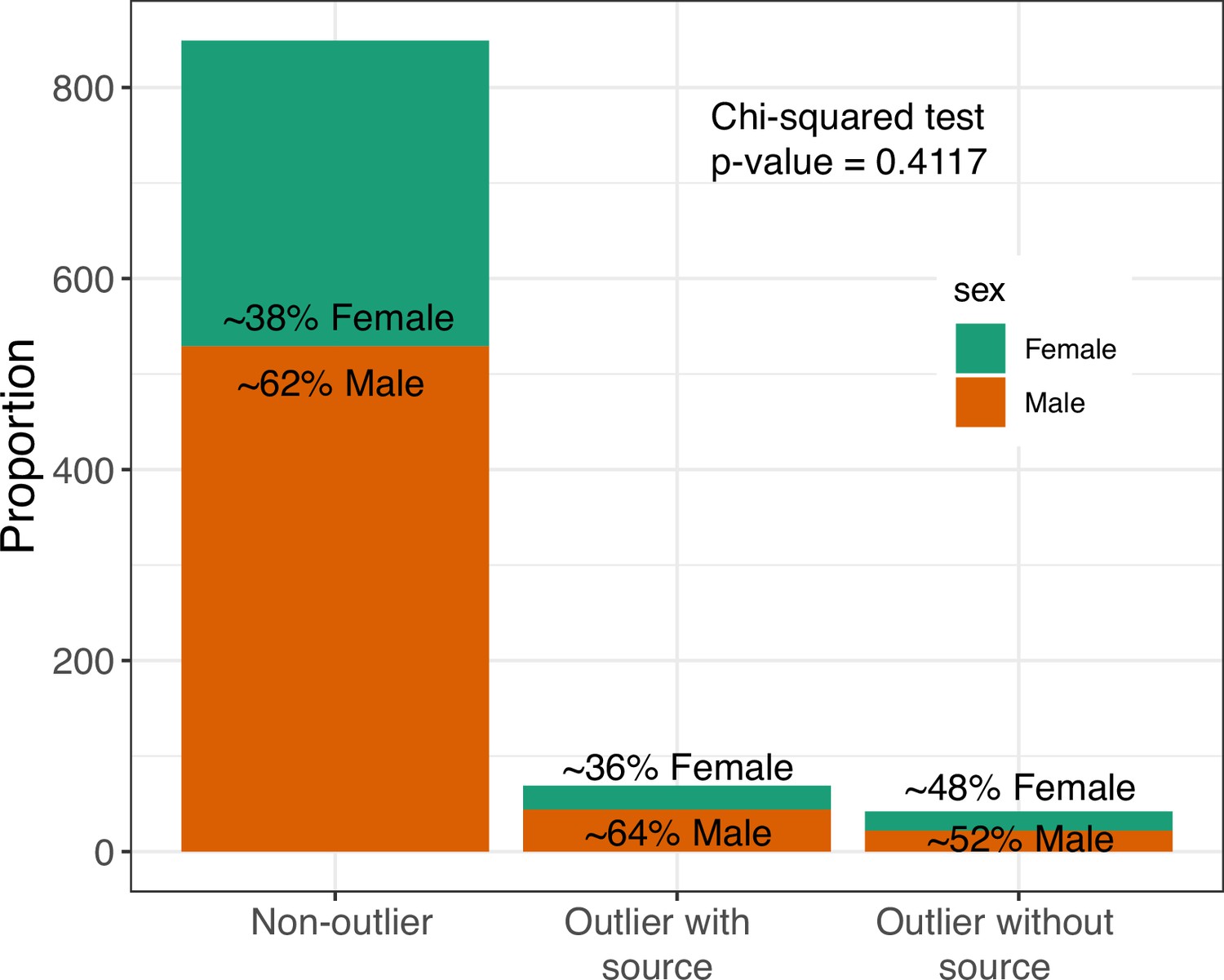
Lack of sex-bias amongst outliers with valid qpAdm sources.
The proportions of males and females do not differ significantly between outlier and non-outlier groups (p=0.4117). When outliers (with and without source) are treated as one group, there is still no significant association with outlier status and sex (p=0.633).
Figure 5—figure supplement 2
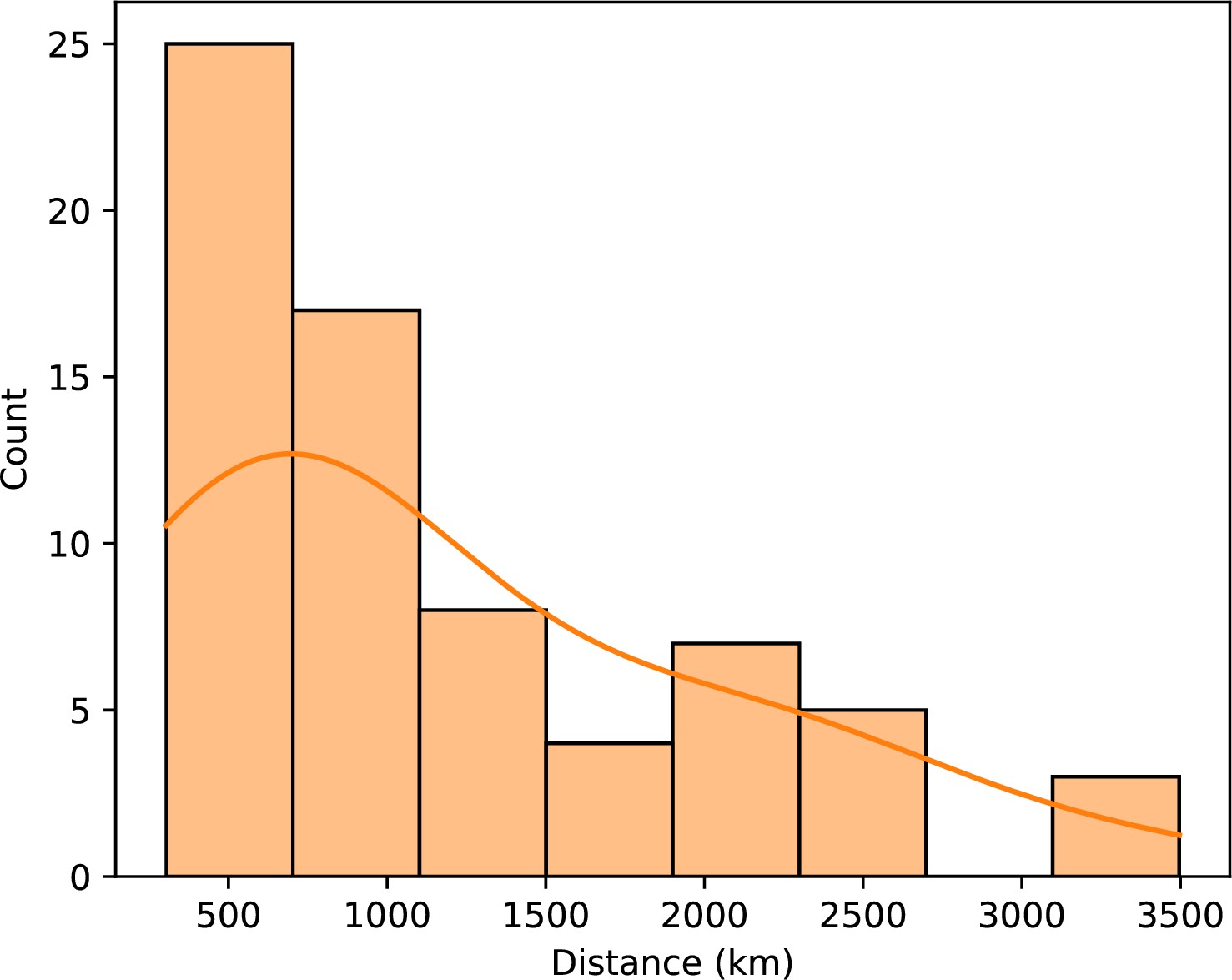
Distances of outliers to their candidate sources.
Geographic distance between the sampling locations of ‘outlier with source’ and the location of their putative source was calculated for each outlier. The mean distance was calculated if there were multiple putative sources.
Figure 5—figure supplement 3
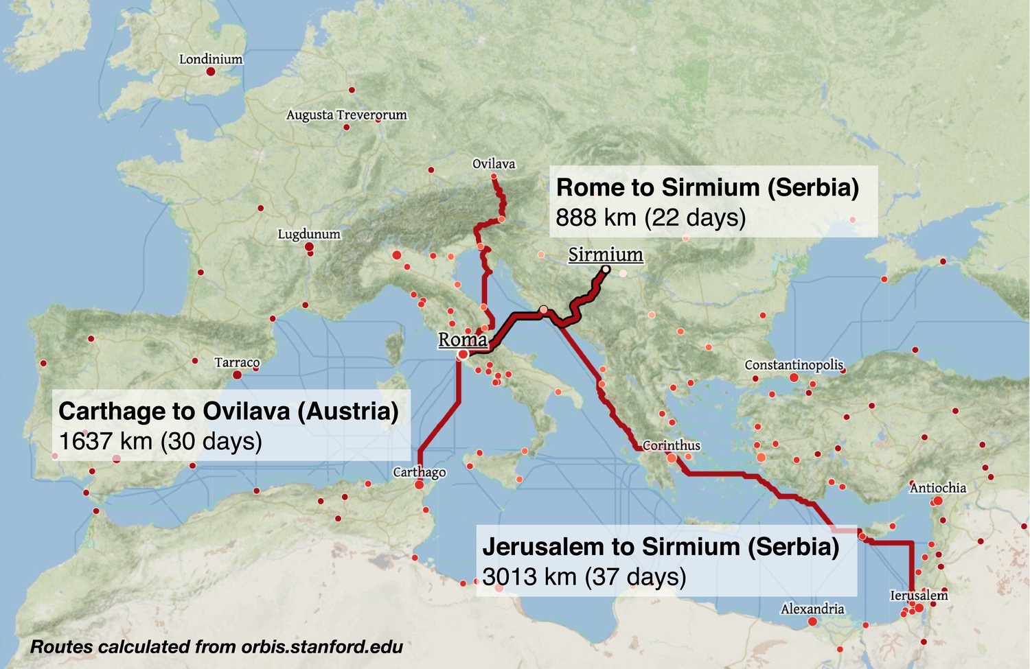
Example routes and travel times across the Roman Empire.
Routes and travel times were approximated using orbis.stanford.edu, a geospatial network model of the Roman Empire. Routes shown are the fastest routes during Summer for civilians, utilizing road, river, coastal sea, and open sea, and by foot if on road. Routes for military individuals (not shown) are marginally faster.
Figure 6
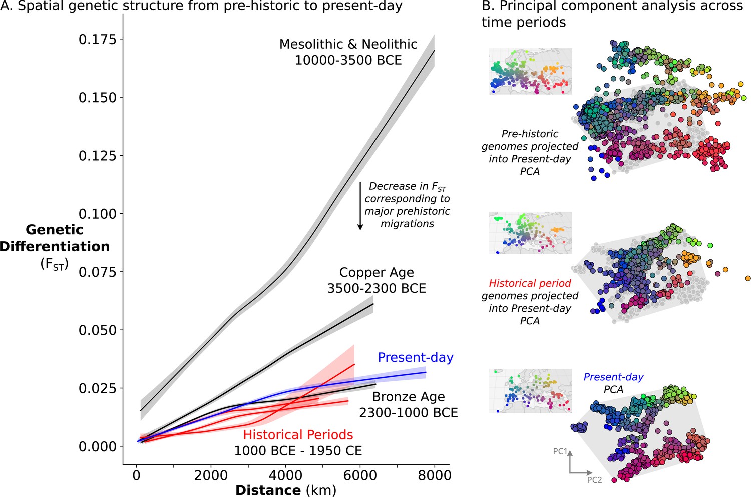
Relatively stable population structure from Bronze Age to present-day.
(A) Overall genetic differentiation between populations (measured by FST) and its relationship to geographical distance (spatial structure) is similar from Bronze Age onward. Confidence intervals were calculated through a bootstrap procedure, using 200 bootstrap replicates. (B) In PC space, each genome is represented by a point, colored based on their origin (for present-day individuals) or sampling location (for historical samples). The PC space is established by present-day samples (bottom), onto which either historical period (middle) or prehistoric genomes (top) were projected. For projections, the present-day samples are shown in gray, and their extent is visualized by a gray polygon.
Figure 7 with 2 supplements
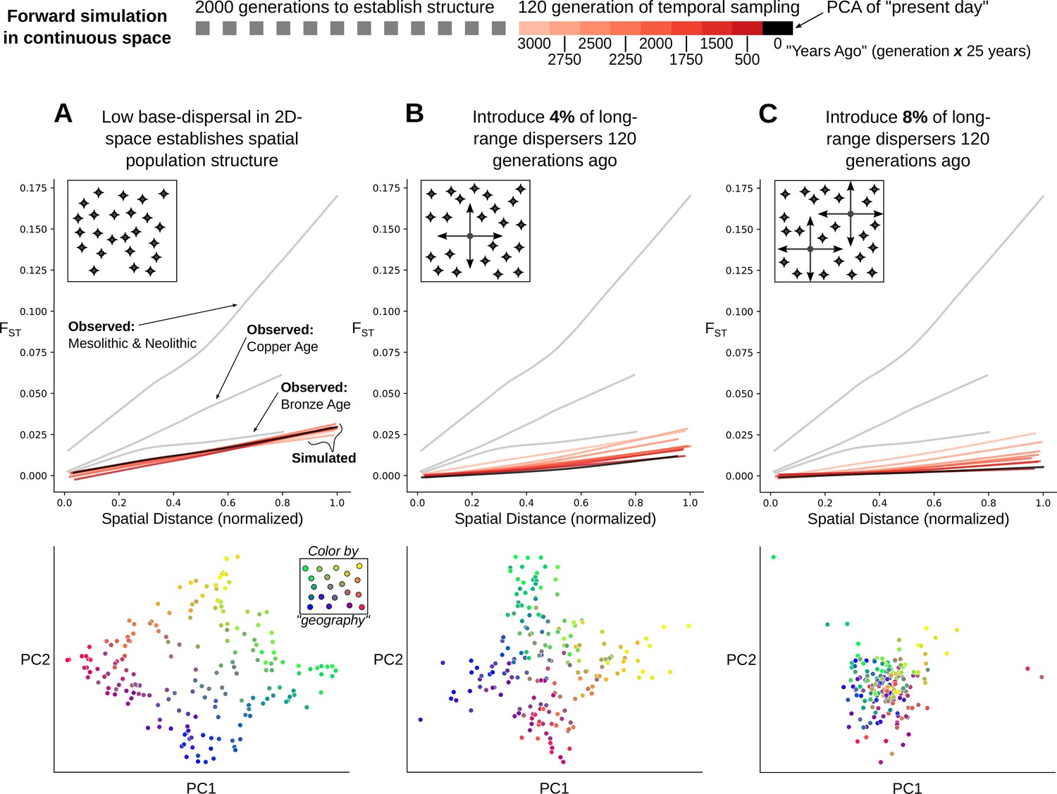
Simulation of population structure with and without long-range dispersal.
(A) A base model of spatial structure is established by calibrating per-generation dispersal rate to generate a maximum FST of ~0.03 across the maximal spatial distance, and visualized using PCA. In addition to this base dispersal, either 4% (B) or 8% (C) of individuals disperse longer distances, and the effect is tracked by analyzing spatial FST through time, as well as PCA after 120 generations of long-range dispersal.
Figure 7—figure supplement 1
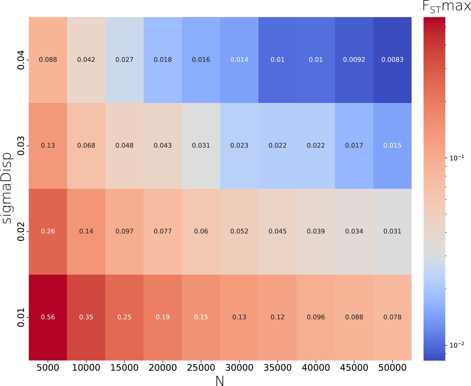
A sigmaDisp - N parameter pair was chosen to closely approximate the observed FSTmax of ~0.03 using grid search across a range of parameter pairs.
We used the pair N=50,000 & sigmaDisp = 0.02 for all other simulations we report.
Figure 7—figure supplement 2
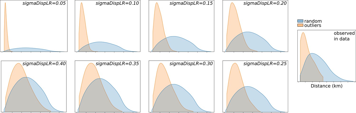
A sigmaDispLR parameter was chosen to qualitatively resemble long-range dispersal distances observed in the data, by comparing the distribution of distances under long-range dispersal (outliers) to randomly chosen distances given the spatial distribution of samples.
We used a value of 0.20 for all other simulations we report.
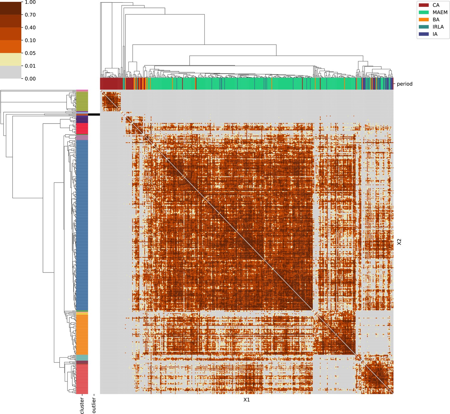
Appendix 1—figure 1
Armenia.
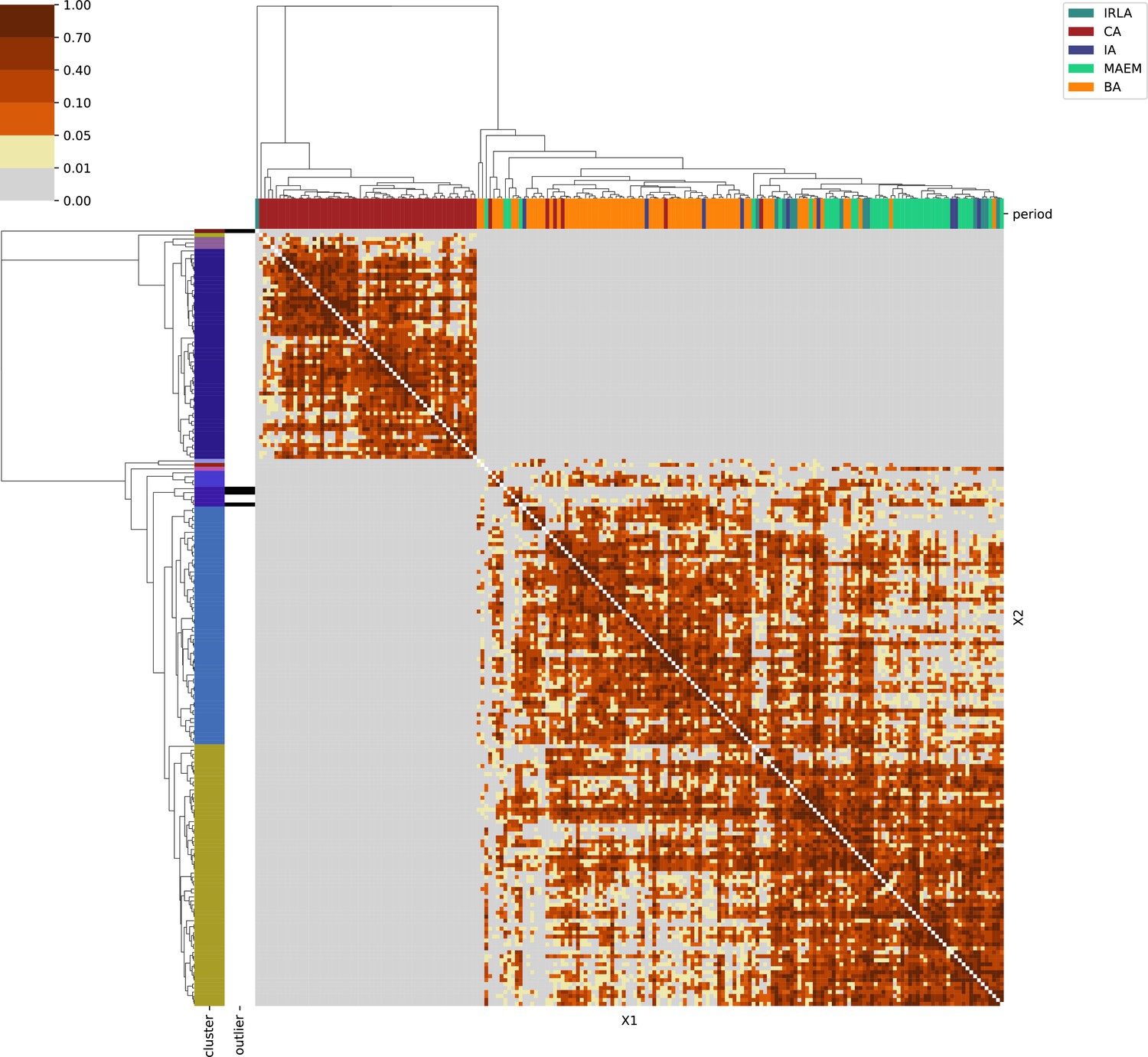
Appendix 1—figure 2
Mainland Italy.
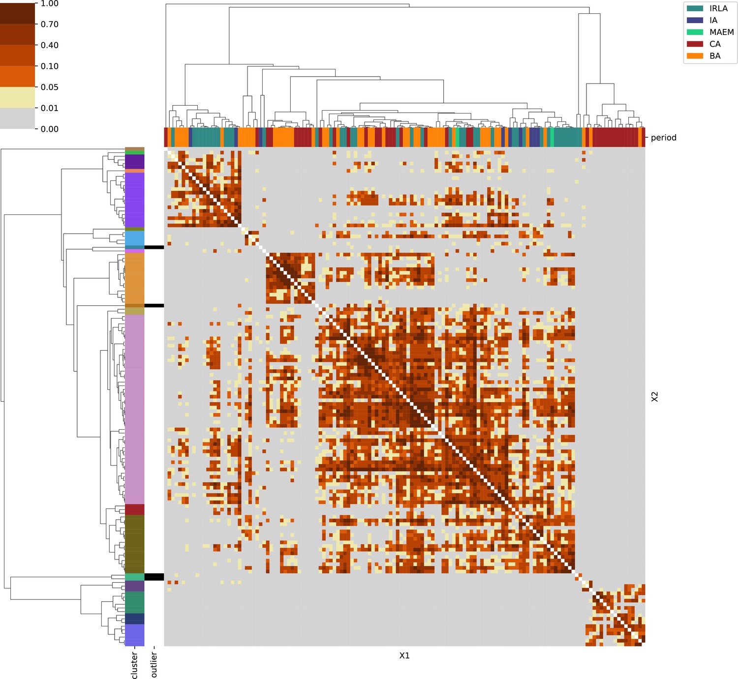
Appendix 1—figure 3
Sardinia.
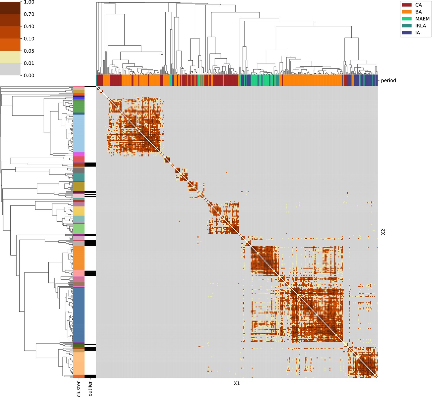
Appendix 1—figure 4
Levant & Egypt.
Appendix 1—figure 5
Southeastern Europe.
Appendix 1—figure 6
Southwestern Europe.
Appendix 1—figure 7
Western Europe.
Appendix 1—figure 8
Northern Europe.
Appendix 1—figure 9
Great Britain & Ireland.
Appendix 1—figure 10
Eastern Central Europe.
Appendix 1—figure 11
Eastern Europe & Steppe.
Appendix 1—figure 12
North Africa.
Author response image 1
SNP coverage comparison between outliers and non-outliers in region-period pairings with “surprising” outliers (t-test p-value: 0.
242).
Author response image 2
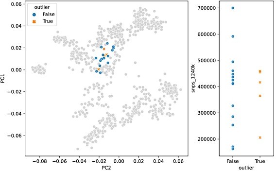
PCA projection (left) and SNP coverage comparison (right) for “surprising” outliers and surrounding non-outliers in Italy_IRLA.
Author response image 3
Projection of qpAdm reference population individuals into present-day PCA.
Author response image 4
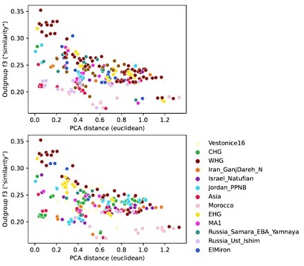
Comparison of pairwise PCA projection distance to outgroup-f3 similarity across all qpAdm reference population individuals.
PCA projection distance was calculated as the euclidean distance on the first two principal components. Outgroup-f3 statistics were calculated relative to Mbuti, which is itself also a qpAdm reference population. Both panels show the same data, but each point is colored by either of the two reference populations involved in the pairwise comparison.
Author response image 5
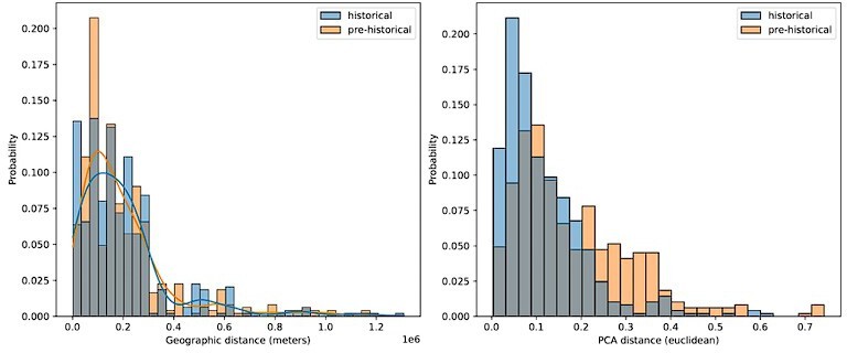
Comparing geographic distance to PCA distance between pairs of historical and pre-historical individuals matched by geographic space.
For each historical period individual we selected the closest pre-historical individual by geographic distance in an effort to match the distributions of pairwise geographic distance across the two time periods (left). For these distributions of individuals matched by geographic distance, we then queried the euclidean distance between their projection locations in the first two principal components (right).
Additional files
-
Supplementary file 1
Archaeological context for sampling locations.
- https://cdn.elifesciences.org/articles/79714/elife-79714-supp1-v1.docx
-
Supplementary file 2
Metadata for all newly reported individuals Supplementary file 3.
- https://cdn.elifesciences.org/articles/79714/elife-79714-supp2-v1.zip
-
Supplementary file 3
AMS and calibration results.
- https://cdn.elifesciences.org/articles/79714/elife-79714-supp3-v1.zip
-
Supplementary file 4
Published samples that contributed to this study.
- https://cdn.elifesciences.org/articles/79714/elife-79714-supp4-v1.zip
-
MDAR checklist
- https://cdn.elifesciences.org/articles/79714/elife-79714-mdarchecklist1-v1.docx
Download links
A two-part list of links to download the article, or parts of the article, in various formats.
Downloads (link to download the article as PDF)
Open citations (links to open the citations from this article in various online reference manager services)
Cite this article (links to download the citations from this article in formats compatible with various reference manager tools)
Stable population structure in Europe since the Iron Age, despite high mobility
eLife 13:e79714.
https://doi.org/10.7554/eLife.79714


