Determining growth rates from bright-field images of budding cells through identifying overlaps
- Centre for Engineering Biology and School of Biological Sciences, University of Edinburgh, United Kingdom
Figures
Figure 1 with 1 supplement
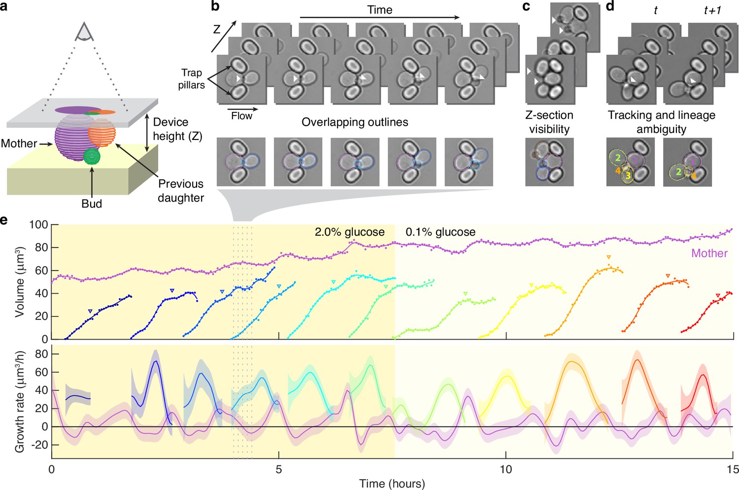
Reliably identifying individual cells makes automatically segmenting label-free cells that bud challenging.
(a) A schematic of a budding cell constrained in a microfluidic device showing how a mother cell can produce a bud beneath the previous daughter. The microscope, denoted by the eye, sees a projection of these cells. (b) A time series of bright-field images of budding yeast trapped in an ALCATRAS microfluidic device (Crane et al., 2014), in which a growing bud (white arrowheads) overlaps with both its sister and mother. On the duplicated images below, we show outlines produced by BABY. (c) Bright-field images of growing buds (white arrowheads) taken at different focal planes demonstrate how the appearance of small buds may change. (d) Cells can move substantially from image to image. Here medium flowing through the microfluidic device causes a cell to wash out between time points and the remaining cells to pivot. We indicate the correct lineage assignment by white arrowheads and the correct tracking by the numbers within the BABY outlines. (e) We show a time series of a mother (purple) and its buds and daughters for a switch from 2% to 0.1% glucose using volumes and growth rates estimated by BABY. Bud growth rates are truncated to the predicted time of cytokinesis (triangles). Shaded areas are twice the standard deviation of the fitted Gaussian process.
Figure 1—figure supplement 1
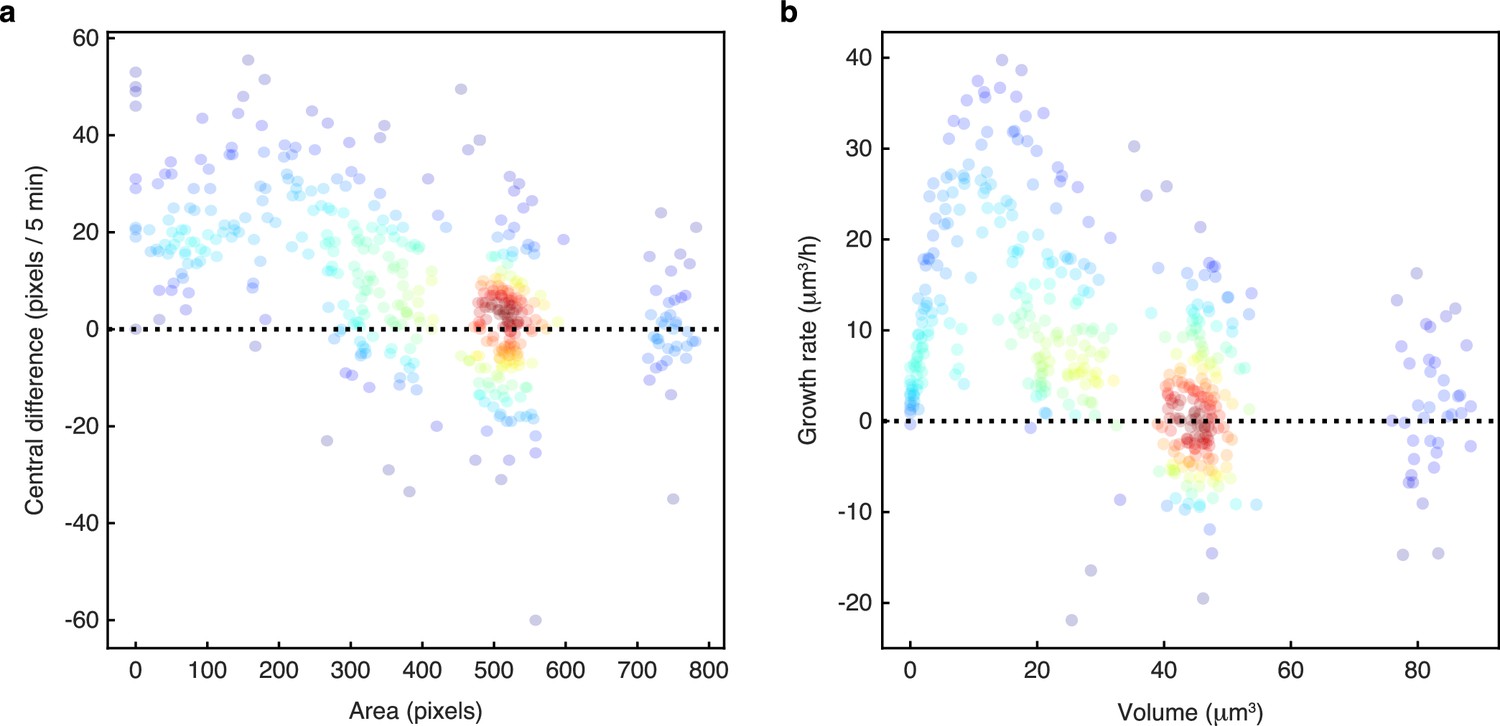
Growth rates are highest for small buds.
We plot growth rates against cell size for nine sets of manually annotated time series of mother-bud pairs randomly selected from microfluidics experiments in four different growth conditions. Growth rates are estimated either as (a) the central difference in mask area or (b) using a Gaussian process fit of the conical volume estimated from the mask. For each pair, we annotated the mother and bud from when the bud appears to when the mother next buds. The points are growth rate and size estimates for each annotated time point, coloured using a kernel density estimate.
Figure 2
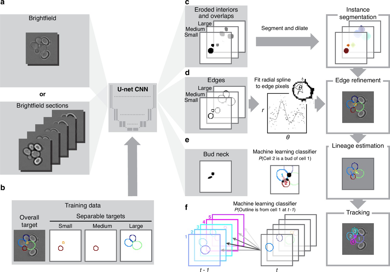
BABY uses multiple bright-field Z-sections, a multi-target convolutional neural network followed by a custom segmentation algorithm, and two machine-learning classifiers to identify cells and their buds reliably from image to image.
(a) Either single or multiple, we typically use five, bright-field Z-sections are input into a multi-target U-net CNN. (b) The curated training data comprises multiple outlines that we categorise by size to reduce overlaps between cells within each category. (c) We train the CNN to predict a morphological erosion of the target cell images, which act as seeds for segmenting instances of cells. (d) We use edge targets from the CNN to refine each cell’s outline, parameterised as a radial spline. (e) We use a bud-neck target from the CNN and metrics characterising the cells’ morphologies to estimate the probability that a pair of cells is a mother and bud via a machine-learning classifier. (f) Another classifier uses the same morphological metrics to estimate the probability that an outline in the previous time point matches the current one.
Figure 3 with 6 supplements
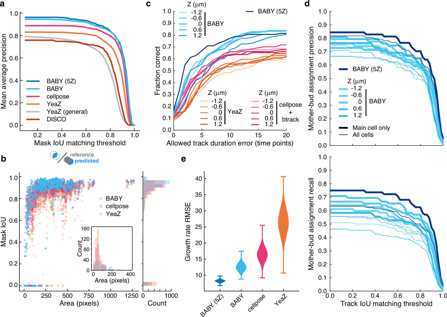
BABY outperforms other algorithms for segmenting, tracking, and particularly for estimating growth rates.
(a) Comparing the intersection-over-union (IoU) score (Methods) between manually curated single cells and those predicted by the BABY, Cellpose, YeaZ, and DISCO algorithms shows that BABY performs best, particularly with five Z sections as input (5Z). We show the performance of the generalist YeaZ model and the Cellpose and YeaZ algorithms retrained on the BABY training data. (b) BABY performs particularly well for smaller cell sizes. Inset: counts of curated cells missed by each algorithm. (c) BABY finds a higher fraction of complete tracks than either YeaZ or Cellpose, an algorithm only for segmentation and trained on BABY data, combined with btrack (Ulicna et al., 2021), a tracking algorithm. We show the results for each Z section separately because BABY is the only algorithm that can use more than one. (d) We show BABY’s precision and recall for correctly assigning mother and bud tracks in the tracking evaluation data set as a function of the threshold for defining matching tracks. Performance is best for the central trapped cell. We are unaware of any other algorithms performing mother-bud assignment directly from bright-field images with which to compare. (e) By accurately detecting and estimating buds with small volumes, BABY also shows the smallest Root Mean Squared Error (RMSE) when comparing predicted bud growth rates with those derived from a manually curated set of time series of randomly selected mother-bud pairs from four different growth conditions. To highlight the importance of segmentation quality for estimating growth rates, we matched outlines to ground truth ignoring any tracking errors. We used 104 bootstraps of 90% of the ground truth data (209 estimates of growth rate from 9 buds) to find the distributions of RMSE.
Figure 3—figure supplement 1
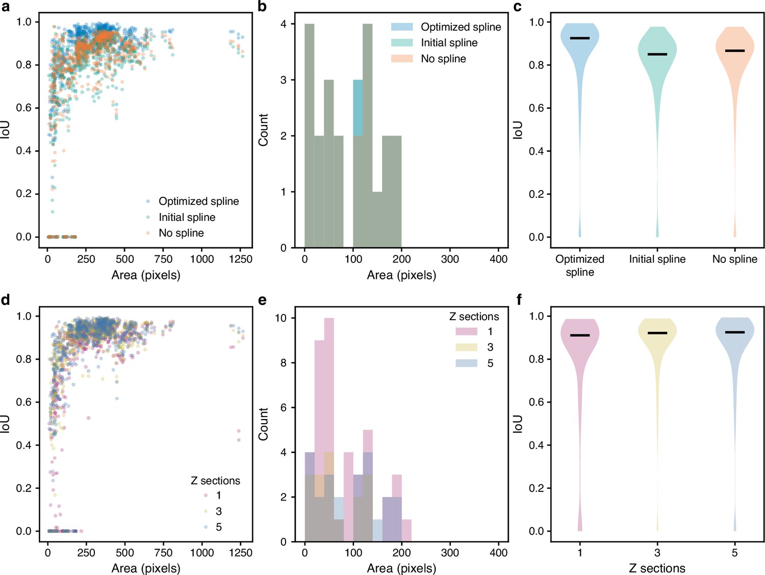
Optimising edges and using multiple Z sections as inputs improves segmentation.
(a–c) We evaluated the intersection over union (IoU) with curated masks for the predictions of selected stages of the BABY algorithm: masks predicted directly from CNN output with appropriate morphological dilation (no spline), preliminary fits of these masks with an equal-angle radial spline (initial spline), or optimised fits of the radial spline to the edge output of the CNN (optimised spline). (d–f) With either one, three, or five bright-field Z sections as input, we found the IoU with curated masks of the full BABY algorithm’s predictions. (a, d) The distributions of the IoU with curated outline area. (b, e) The distributions of curated outline areas for missed predictions, with an IoU of zero. (c, f) Violin plots summarising the IoU distributions. The black horizontal line is the median.
Figure 3—figure supplement 2

BABY is competitive with existing algorithms for segmenting microcolonies.
We show the intersection over union (IoU) with manually annotated masks from the YeaZ bright-field training data Dietler et al., 2020 for predictions from BABY (single Z section), Cellpose, and YeaZ. All were trained on both the BABY training data and an additional three images from the YeaZ training data. We show too predictions from the default YeaZ model trained on all evaluation data, labelled as YeaZ (general), and from a generalist Cellpose model, labelled cellpose (general).
Figure 3—figure supplement 3
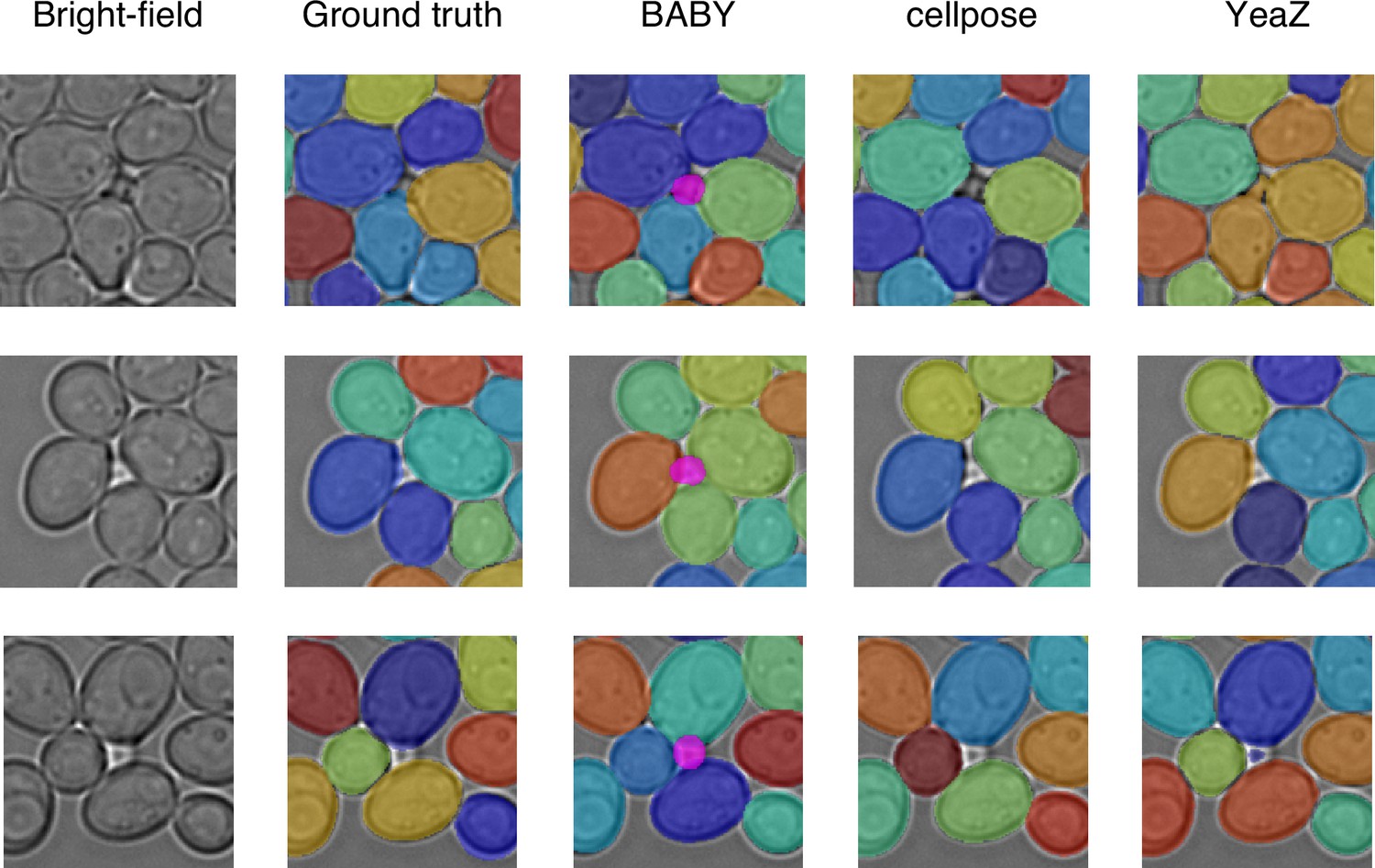
BABY detects buds that were missing in the YeaZ training images.
We show examples of buds detected by BABY (bright magenta overlay) in cropped bright-field images of a microcolony in the YeaZ training data [Dietler et al., 2020]. Although reported as false positives and off the focal plane, we disagree here with the ground truth and would annotate these objects as buds. YeaZ, with its own standard bright-field model that includes these images in its training data, annotated one of the buds; Cellpose trained on the same data as BABY misses all.
Figure 3—figure supplement 4

BABY produces fewer missing tracks than existing other algorithms.
We compare the distribution of single-cell track IoUs between manually curated and predicted tracks – the number of time points where the masks match relative to the total number of time points in both tracks. We focus on performance for a single Z section (the focal plane and most central one), comparing the single-Z BABY algorithm, YeaZ [Dietler et al., 2020], and tracking by the btrack algorithm [Ulicna et al., 2021] on outlines segmented by Cellpose [Pachitariu and Stringer, 2022]. Unassigned ground-truth tracks have an IoU of zero. They typically arise when two ground-truth tracks appear as a single predicted track. We exclude unassigned predicted tracks.
Figure 3—figure supplement 5
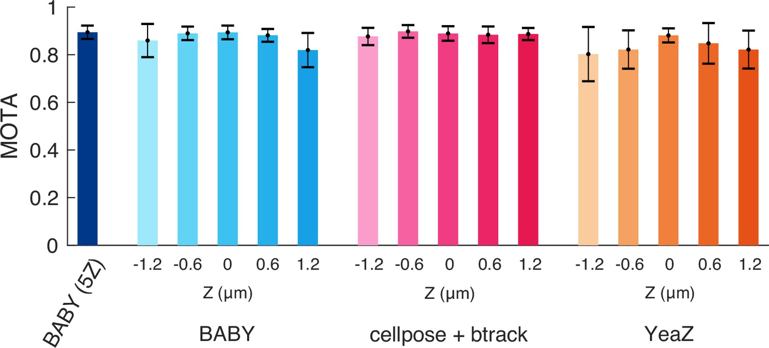
All algorithms tested track similarly when assessed with a generalised metric.
We show mean Multiple Object Tracking Accuracies (MOTA) [Bernardin et al., 2006] for each Z section of our test data for BABY, the btrack algorithm [Ulicna et al., 2021] on outlines segmented with Cellpose [Pachitariu and Stringer, 2022] – the top performer, and YeaZ [Dietler et al., 2020]. We include too the five-Z section BABY algorithm (5Z). Error bars are standard error of the mean ().
Figure 3—figure supplement 6
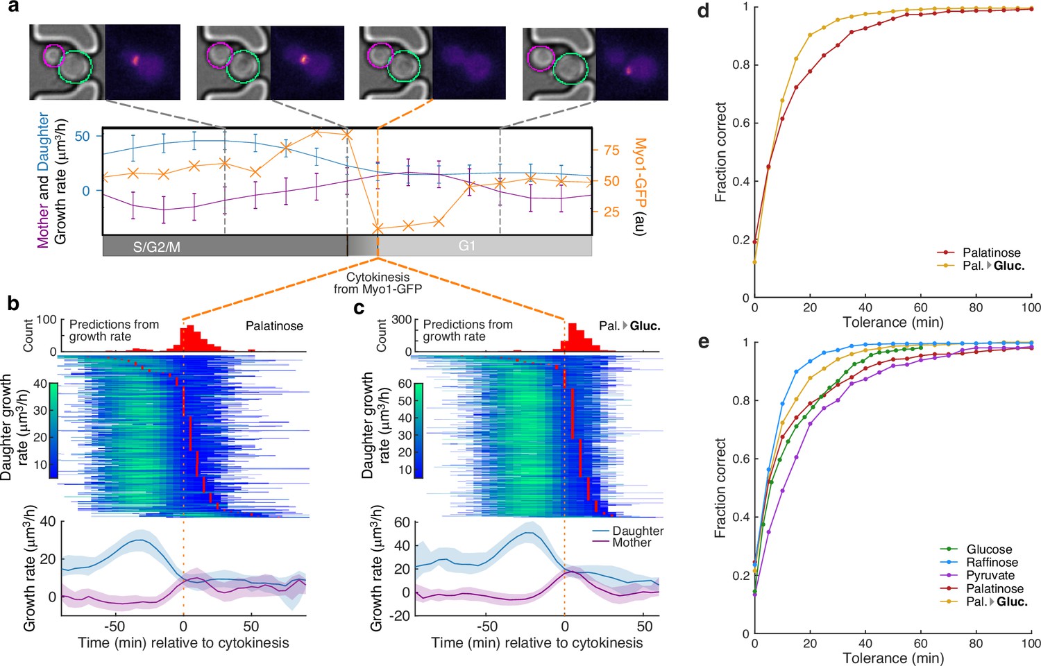
A peak in the bud’s growth rate predicts cytokinesis.
(a) Using MYO1-GFP as a marker, we split individual cell cycles of mother cells into G1 and S/G2/M phases. We show bright-field and fluorescence images for a representative cell during one cell cycle. Myo1’s fluorescence at the bud neck abruptly disappears at cytokinesis. The cell’s growth rate (purple) and that of its bud (blue) are shown with a measure of Myo1’s localisation (orange). We estimate the point of cytokinesis from the drop in Myo1 fluorescence (orange dashed line). (b) Horizontal lines with shading indicating growth rates show the time series for 388 buds or daughters of 318 cells growing in 2% palatinose. We align cells by the drop in Myo1’s fluorescence and plot the corresponding median growth rates of mother and bud below, with the interquartile range shaded. Red points in the time series mark the time of cytokinesis predicted from the bud’s growth rate, and we show their distribution above. (c) The time series for 850 buds or daughters of 520 cells growing in 2% glucose after a switch from palatinose (Pal. → Gluc.). (d) The fraction of cytokinesis events whose timing was correctly identified by our method of predicting cytokinesis directly from growth rate. We find the ground-truth values using Myo1-GFP ( for 2% palatinose; for 2% glucose after switching from palatinose). (e) Accuracy of our method for ground-truth data estimated using a tagged nuclear marker (Nhp6A-mCherry), which reports the start of anaphase ( for 2% glucose; for 2% raffinose; for 2% pyruvate; for 2% palatinose; and for 2% glucose after switching from palatinose). We assume a fixed 20-min delay from the onset of anaphase to cytokinesis [Leitao and Kellogg, 2017].
Figure 4 with 1 supplement
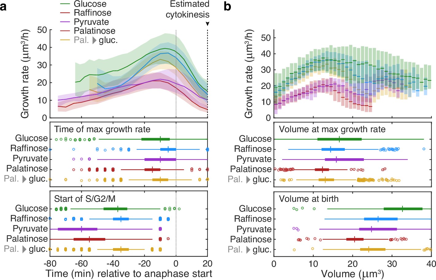
Buds reach similar sizes as their growth rate peaks regardless of carbon source.
(a) Although buds grow faster in richer media, the time of the maximal growth rate relative to the start of anaphase is approximately constant, unlike the duration of the mothers’ S/G2/M phases. We grew cells in 2% glucose (data for 1014 cell cycles), 2% raffinose (803 cycles), 2% pyruvate (270 cycles), 2% palatinose (393 cycles), or in 2% glucose after a switch from palatinose (pal. → gluc.; 842 cycles). We show median bud growth rates with the interquartile range shaded and estimate the timing of anaphase from a fluorescently tagged nuclear marker (Nhp6A-mCherry; Appendix 6) and the start of S phase by when a bud first appears. (b) Binning median bud growth rates according to volume, with the interquartile range shaded, shows that the bud volumes when their growth rate is maximal are more similar in all carbon sources than those at birth, taken as 20 min after start of anaphase (Leitao and Kellogg, 2017) .
Figure 4—figure supplement 1
Growth rates estimated with BABY show expected correlations with volume.
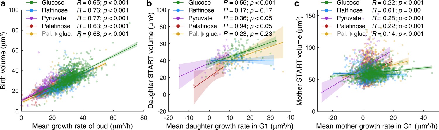
(a) The mean growth rate of a bud from first detection to birth correlates with its volume at birth for buds growing in either 2% glucose, 2% raffinose, 2% pyruvate, 2% palatinose, or 2% glucose after a switch from palatinose (Pal. → gluc). We define birth to be when cytokinesis completes as estimated from an Nhp6A-mCherry marker – Appendix 6. (b) The mean growth rate of a daughter cell during its first G1 phase, from birth to START, correlates with its volume at START. We define START when the daughter’s first bud appears. In our microfluidic devices, the medium washes most daughters away before they can bud. (c) The mean growth rate of a mother during G1, from birth of a daughter to START, shows less correlation with its volume at START. We define START by when the mother’s next bud appears.
Figure 5 with 1 supplement
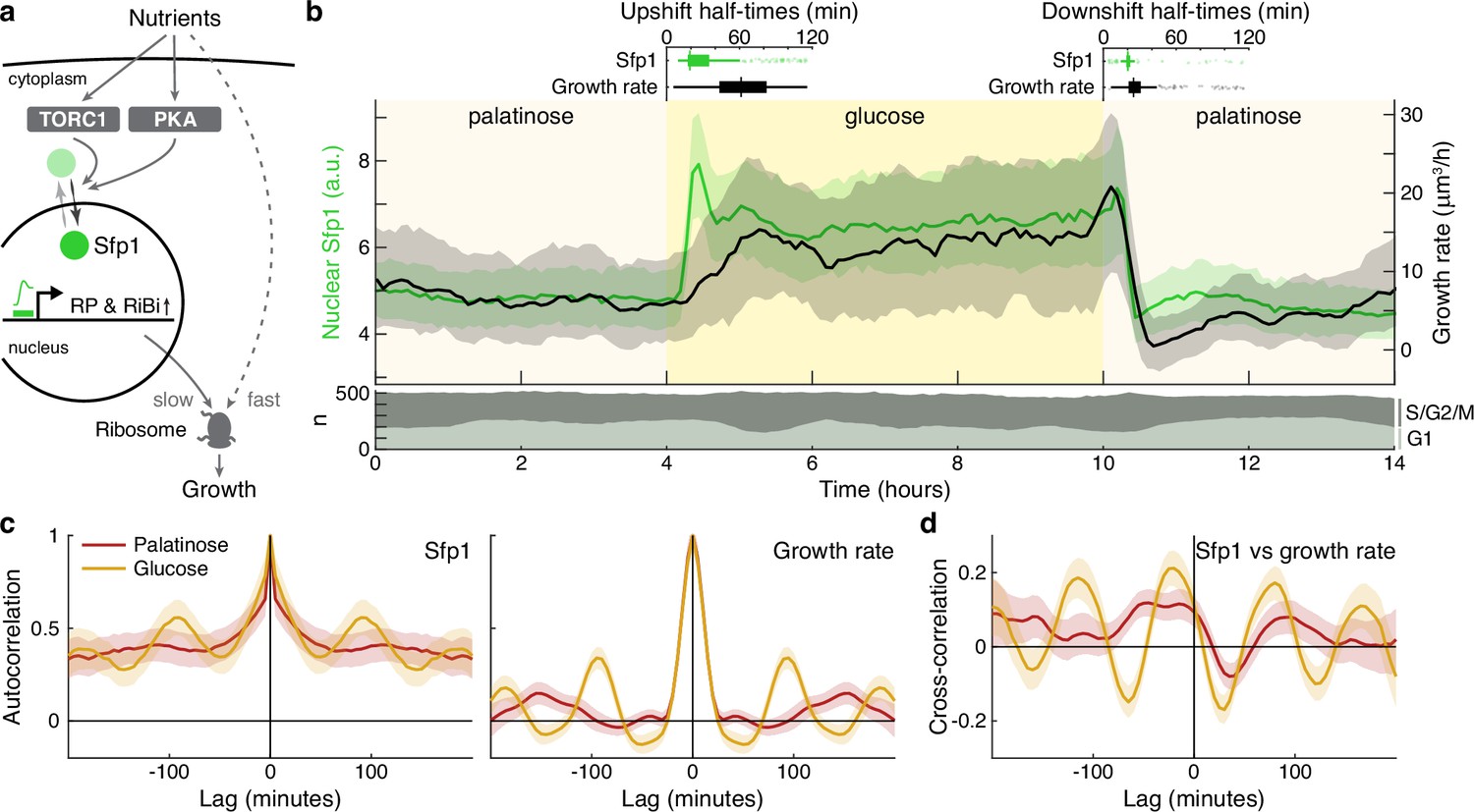
The translocation dynamics of the ribosomal regulator Sfp1 anticipate changes in single-cell growth rates.
(a) The transcription factor Sfp1 is phosphorylated by TORC1 and likely PKA when extracellular nutrients increase and moves into the nucleus, where it promotes synthesis of ribosomes and so higher growth rates. (b) Growth rate follows changes in Sfp1’s nuclear localisation if nutrients decrease but lags if nutrients increase. We show the median time series of Sfp1-GFP localised to the nuclei of mother cells (green) and the summed bud and mother growth rates (black) for cells switched from 2% palatinose to 2% glucose and back. Shading shows interquartile ranges. We filtered data to those cell cycles that could be unambiguously split into G1 and S/G2/M phases by a nuclear marker, and we display the number in each phase in the lower plot. Above the switches of media, we show box plots for the distributions of single-cell half-times: the time of crossing midway between each cell’s minimal and maximal values. (c) The mean single-cell autocorrelation of nuclear Sfp1 and the summed mother and bud growth rates are periodic because both vary during the cell cycle. We calculate the autocorrelations for constant medium using data four hours before each switch (Appendix 7). Shading shows the 95% confidence interval. (d) The mean cross-correlation between nuclear Sfp1 and the summed mother and bud growth rate shows that fluctuations in Sfp1 precede those in growth, with the correlation peaking at negative lags.
Figure 5—figure supplement 1
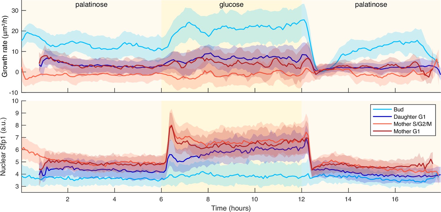
Irrespective of cell cycle phase, growth rates transiently drop for a shift to a poorer carbon source.
We show time series of median growth rate (upper panel) and median Sfp1-GFPlocalisation (lower panel) across different cell-cycle phases for a switch from 2% palatinose to 2% glucose and back. We used a Nhp6A-mCherry reporter to identify cytokinesis – Appendix 6 – and so partitioned the time series into cell-cycle phases: G1 phase for the daughter is from cytokinesis up to BABY detecting its first bud; S/G2/M phase for the mother is from budding to cytokinesis; and its G1 phase is from cytokinesis to budding. The shading shows the interquartile range.
Figure 6 with 1 supplement
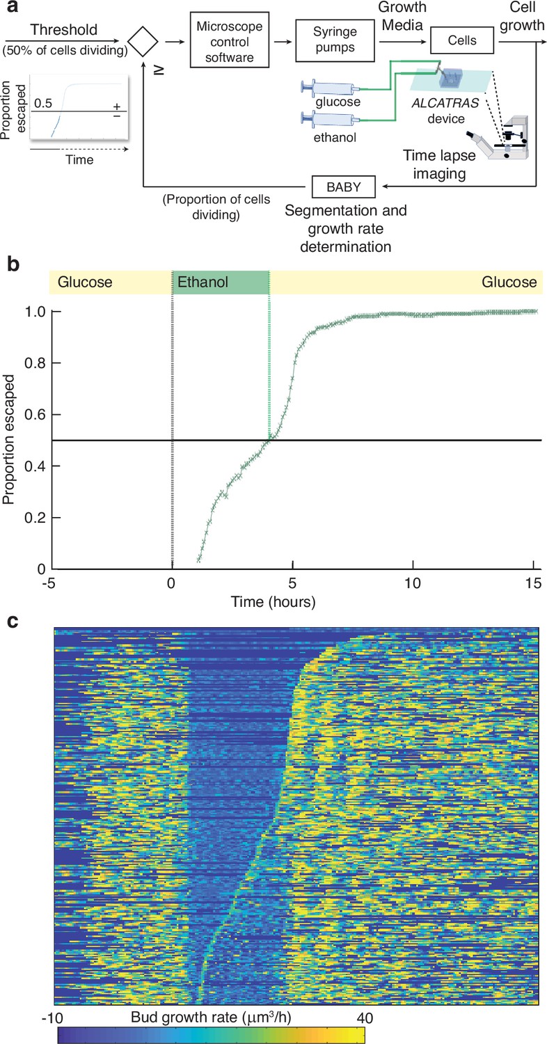
BABY allows growth rate to be used as a variable for real-time control.
(a) By running BABY in real time during a microscopy experiment, we are able to use the cells’ growth rate to control changes in media. Following 5 hr in 0.5% glucose, we switch the extracellular medium to one containing 2% ethanol, a poorer carbon source, and cells arrest growth. The images collected are analysed by BABY to determine growth rates. When the majority of cells have resumed dividing, detected by the growth rate of at least one of their buds or daughters exceeding 15μm3/hr, the microscopy software triggers a change in pumping and returns glucose to the microfluidic device. (b) The fraction of cells that have escaped the lag and resumed dividing increases with the amount of time in ethanol. All cells divide shortly after glucose returns. (c) The growth rates of the buds for each mother cell drop in ethanol and resume in glucose. Each row shows data from a single mother cell with the bud growth rate indicated by the heat map. We sort rows by the time each cell resumes dividing in ethanol, with the bottom rows showing the 50% that re-initiated growth.
Figure 6—figure supplement 1
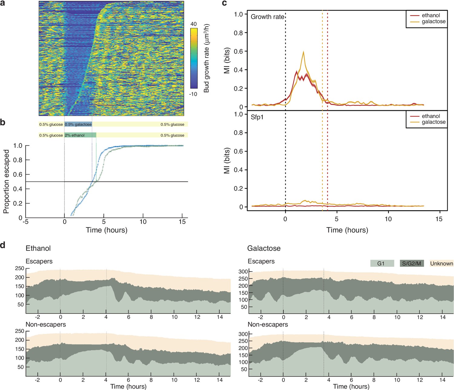
Changing experimental protocols in real time using growth rates.
(a) A heat map showing the bud growth rates calculated in real time for an experiment where the medium changes from glucose to galactose, rather than the ethanol of Figure 6. We sort rows representing mother cells by the time each cell resumes dividing, with cells resuming later at the top. We indicate the corresponding time on the plot below. (b) Cells are slow to resume division, or “escape”, following the switch to 2% ethanol (green) compared to 0.5% galactose. (c) The growth rate but not Sfp1’s localisation is predictive of whether cells escape. We plot the mutual information between cells labelled as either escapers or non-escapers and the time series of either bud growth rate or Sfp1’s localisation. We estimated the mutual information using the decoding method Granados et al., 2018 for a sliding time-window of 100 minutes and show the mean and, with shading, the 95% confidence interval of 100 bootstraps. Decoding was by a gradient-boosting classifier trained on the time-window data concatenated with both Fourier-transformed and rank-ordered versions of the same data. (d) Cells accumulate in G1 while in the poorer carbon source, and their cell cycles appear to synchronise– notice the periodic waves of the proportions of G1 cells once glucose is re-introduced. The dotted lines mark media transitions.
Appendix 1—figure 1
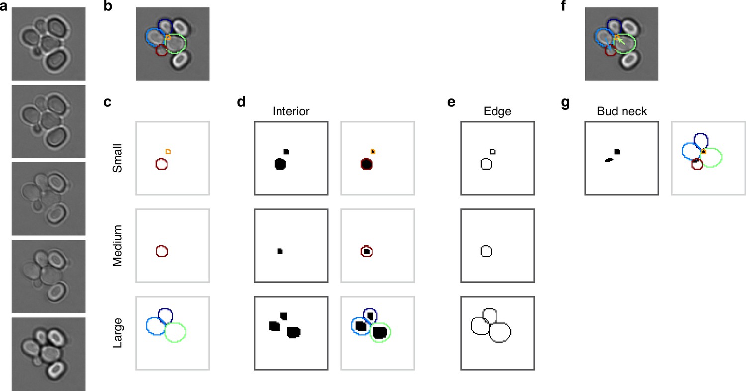
Mapping cell instances to semantic targets of a CNN.
(a) Bright-field Z-sections of cells trapped in an ALCATRAS device. (b) Curated cell outlines overlaid on one bright-field section. (c) BABY separates outlines into categories by size, with each category having some overlap with neighbouring ones. Here the red outline in the medium category appears too in the small category. (d) Cell-interior targets for the CNN are the cell masks generated after different rounds of morphological erosions appropriate for each size category: no erosion for small cells, four iterations for medium, and five for large. On the right, we show the outlines overlaid on the target masks. (e) The CNN’s edge targets are the outlines for each size category. (f) The curated cell outlines of b, but with arrows to show the lineages assigned during curation. (g) Using these curated lineages, we define the CNN’s ‘bud neck’ target as the overlap of the bud mask with a morphological dilation of the mother mask (right).
Appendix 1—figure 2
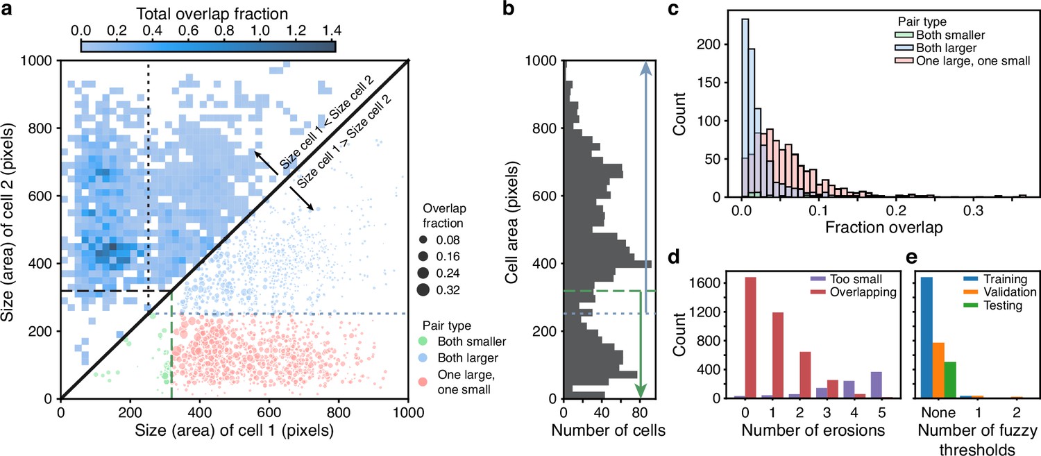
BABY reduces overlaps between cells through categorising cells by size.
(a) Upper triangle: plotting the overlap fraction for each pair of cells – the intersection over union of their bit masks, shows that the majority of overlaps occur for cells of different sizes. Almost all overlaps have the size of cell 2 greater than the size of cell 1 and lie off the diagonal. Lower triangle: With a single fuzzy size threshold, cells in the small category have sizes less than the upper threshold (; dashed line), and cells in the larger category have sizes greater than the lower threshold (; dotted line). We show the overlap fraction by the size of the dot. Within each category (green and blue dots), small overlap fractions dominate; between the two categories (red dots), large overlaps dominate. By converting the bit masks into two binary images, one for each size category, rather than a single binary image, we therefore eliminate most of the substantial overlaps. (b) The distribution of all mask areas in the same training data for comparison. We indicate the size thresholds as in a. (c) The distributions of overlap fractions for mask pairs grouped using the fuzzy size threshold of a. We omit pairs that do not overlap for clarity. (d) Applying morphological erosions of the cell masks reduces the number of overlapping cell pairs, but generates smaller masks. We judge masks with areas below 10 pixels squared to be too small. (e) The numbers of overlapping cell pairs remaining from the training, validation, and test sets either before, denoted None, or after splitting into size categories and applying an optimised number of erosions.
Appendix 1—figure 3
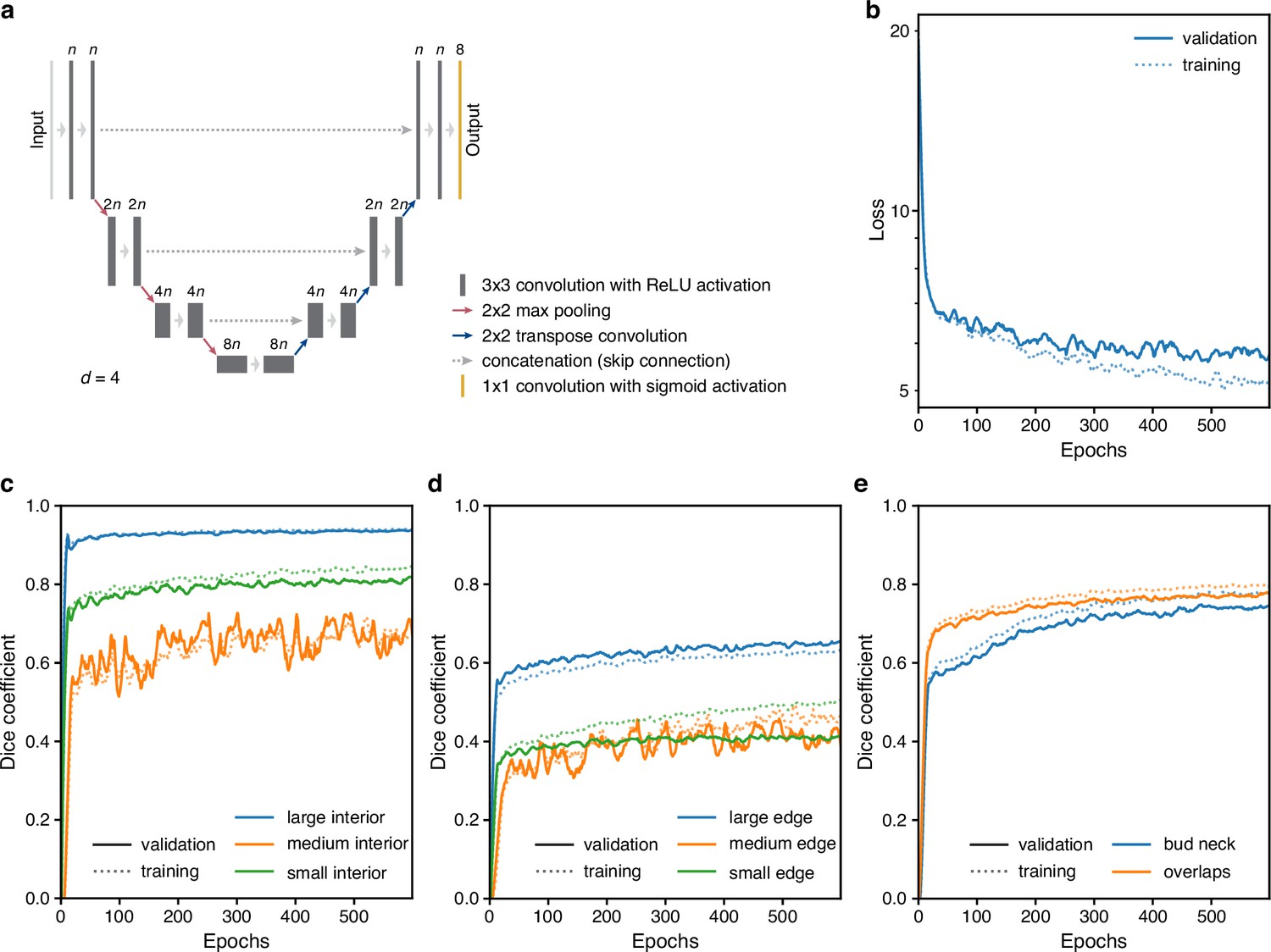
Training performance of the multi-target U-Net.
(a) A schematic of a U-Net architecture with depth . The labels above the convolution operations indicate the number of output filters as a multiple of . Layer heights indicate reduction in image size with network depth. (b) Loss for the fully trained 5Z model U-Net with hyperparameters chosen from training trial giving the lowest final validation loss: a U-Net with depth , filter factor , and batch normalisation. (c–e) Performance of (c) interior, (d) edge and (e) bud neck, and overlap targets by the U-Net of b decomposed into the three different size categories when possible. The Dice coefficient reports similarity between prediction probabilities and target masks with a value of 1 indicating identity. For two sets and , the Dice coefficient is .
Appendix 1—figure 4

Segmenting overlapping cell instances from the CNN’s output.
(a) A flow chart summarising the post-processing for identifying individual instances from the CNN’s multi-target output. Here and below, we show results using the five Z sections of Appendix 1—figure 1 as input to the CNN, and one of which we repeat here. (b) The probability maps output by the CNN for the interiors of small, medium, and large cells. (c) Bit masks obtained by thresholding on the CNN’s output. Darker shading shows bit masks before we dilate each instance to compensate for the erosion applied when generating the training targets. Colour indicates distinctly identified instances. (d) We show the initial, equiangular radial splines proposed for each instance overlaid on the dilated bitmasks from c, with the rays defining placement of the knots as spokes. (e) The same initial proposed radial splines overlaid on the edge target probability maps output by the CNN. (f) The radial splines after optimisation to match edge probabilities. The outline in the medium size category is detected as a duplicate and not optimised.
Appendix 1—figure 5
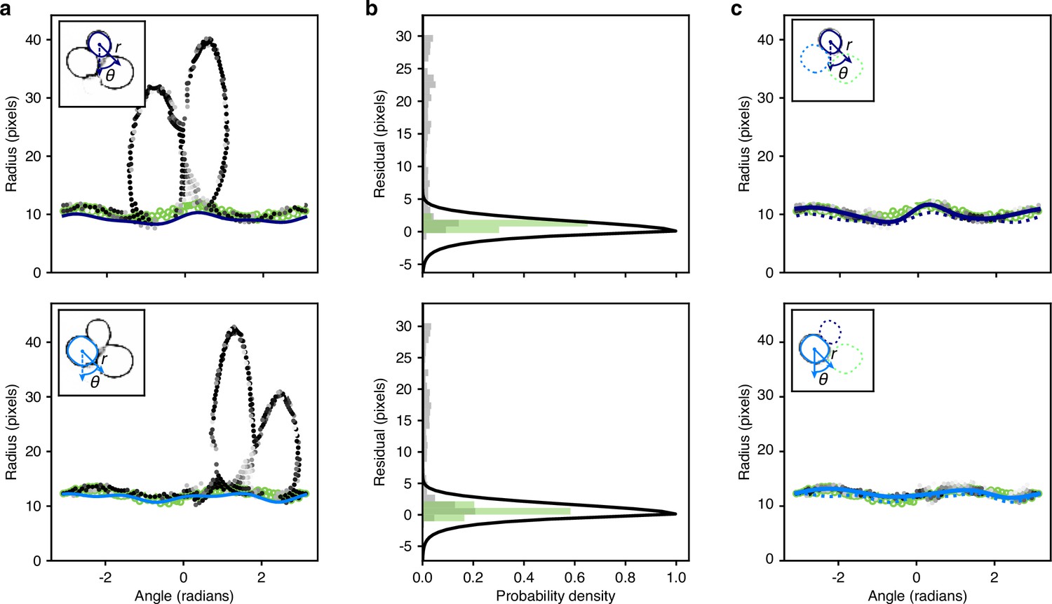
Optimisation of the radial spline to fit the predicted edge.
(a) We show the rdge pixels predicted by the CNN in polar coordinates for two different instances in the top and bottom panels. Darker shading indicates a higher probability of being an edge. Open green circles are the manually curated ground truth. Solid lines are the initial radial splines estimated from the interiors predicted by the CNN. Insets show the predicted edge in cartesian coordinates with the instance providing the origin marked by its initial outline and the indicated polar coordinates. (b) We plot the binned residuals of the predicted edge pixels with the initial radial spline for the examples ofa. The algorithm considers only edge pixels with probability greater than 0.2. Binned residuals for the ground truth are in green. Black lines show the function used to re-weight pixel probabilities for each instance. (c) As for a, but after the edge pixels have been re-weighted for each instance. Solid lines indicate the optimised radial spline. We show the outline favoured by the instance-association probability as a solid line in the inset; disfavoured outlines are dashed.
Appendix 2—figure 1
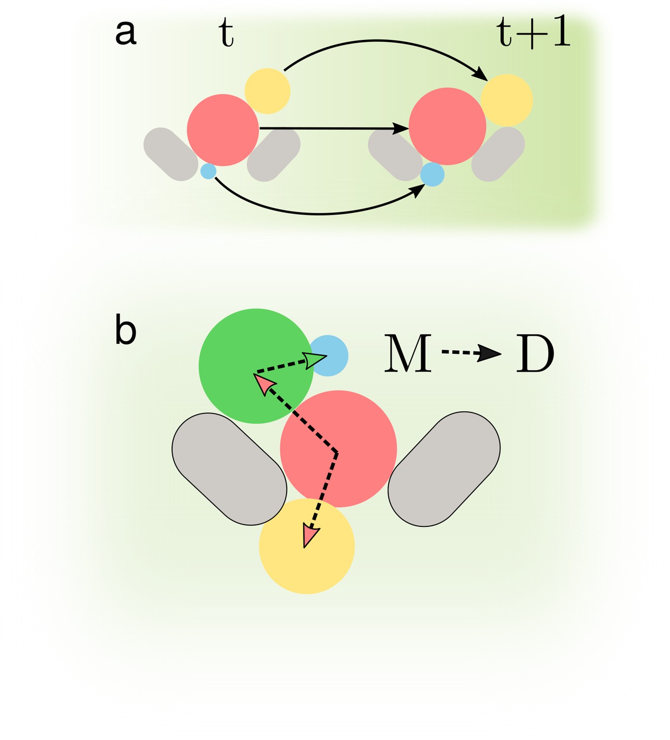
Determining accurate lineages requires solving two independent tasks.
(a) We must identify cells across time points regardless of how they grow and move within the images. (b) We have to find the mother-bud relationship between cells at every time point.
Appendix 2—figure 2
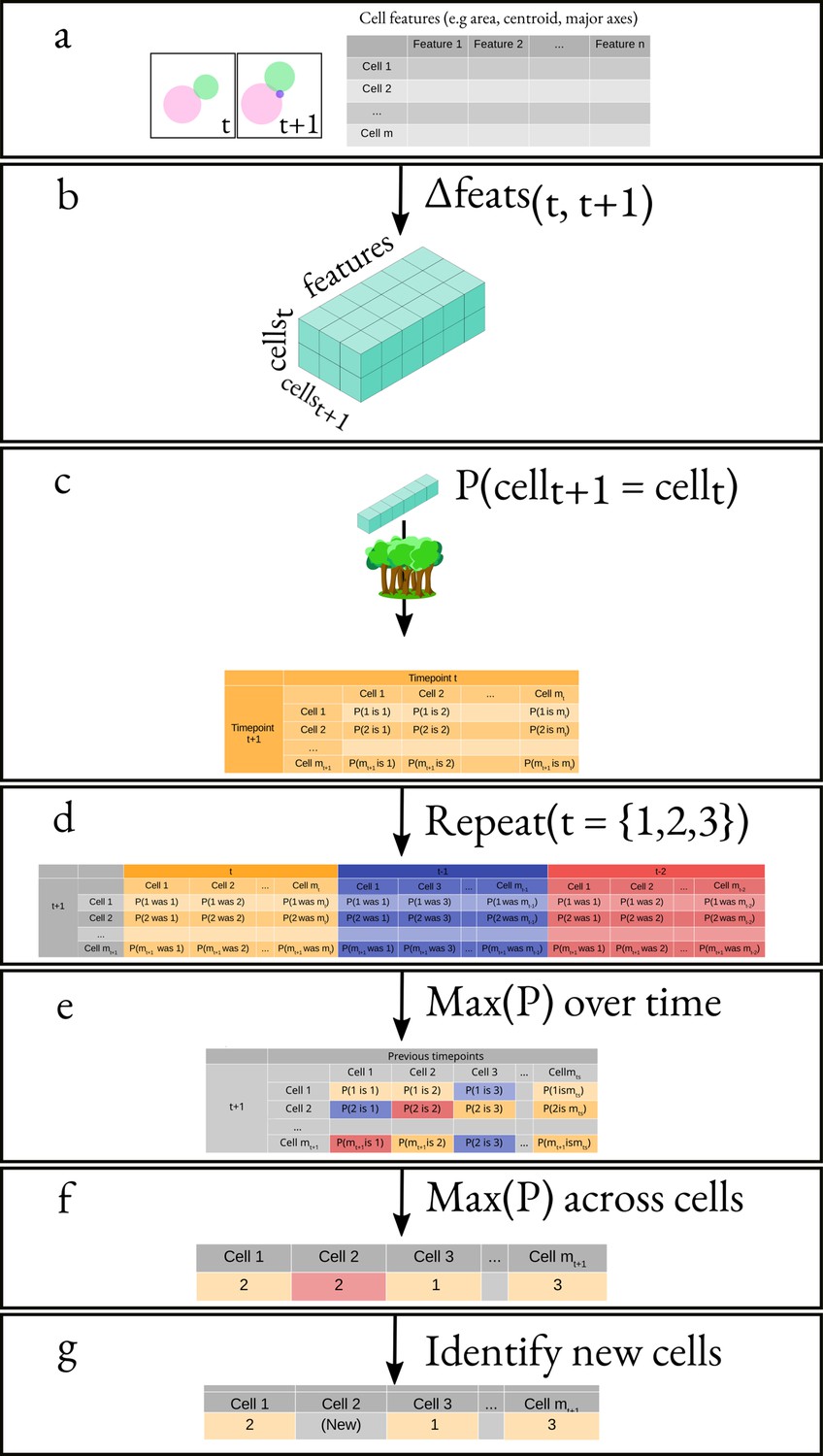
Overview of the algorithm for tracking cells.
(a) We obtain the attributes of all cells at times and . This results in two matrices of shape and , where mx is the number of cells at time and is the number of attributes. (b) We generate a feature vector for every cell pair by subtracting, element-wise, the attributes of all cells at time from the attributes of all cells at time . (c) We apply a classifier to the feature vector corresponding to each pair of cells. (d) We repeat the same process but using and instead of . (e) We pick the maximal probability for every pair of cells over all the probability matrices. (f) We apply our cell-labelling algorithm to assign cell pairs (g) Finally, we use a threshold to identify new cells.
Appendix 2—figure 3
The importance of the features used by the Random Forest classifier for tracking cells between time points.
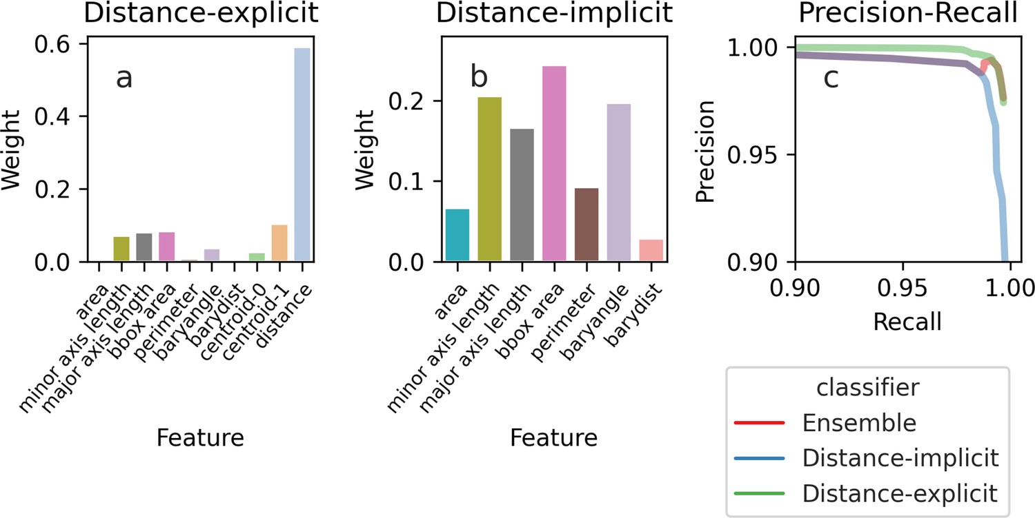
Depending on the features we use, the feature weights, a measure of their importance, are more evenly spread. (a) If we train the classifier using features that explicitly include distance-dependence, distance drives the decisions, and the remaining features are only used for marginal cases. (b) If we train the classifier using distance-implicit features, however, the weights are more uniform. (c) The precision-recall curve shows high accuracy for both sets of features.
Appendix 2—figure 4
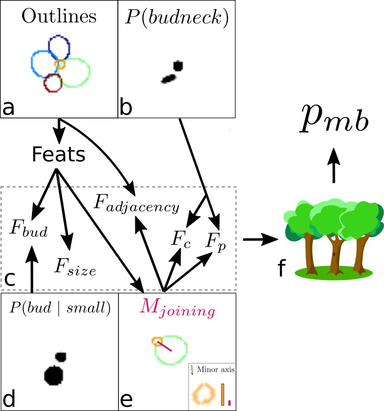
Overview of the algorithm for assigning lineages.
(a, b) We start from the cell outlines and the CNN’s predicted probabilities of a pixel being a bud neck for small cells. Different colour intensities show the probabilities with white denoting zero probability. (c) Composite features used by the classifier to solve the task. (d) The probability of small cells being a bud. (e) An intermediate element of assigning lineages is defining – the red line, actually a rectangular box. (f) Feeding the features into a trained random forest model returns the probability of a pair of cells being a mother and bud.
Appendix 4—figure 1
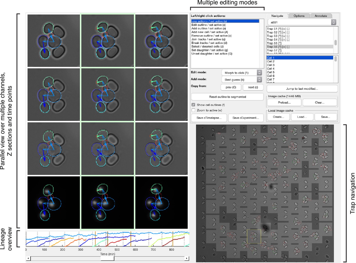
Main features of the graphical user interface used for annotation.
We developed a custom graphical user interface (GUI) in Matlab to annotate efficiently overlapping cell instances, tracks and lineages over long time courses. The screen-shot shows the GUI in its horizontal layout with three bright-field sections and a fluorescence channel selected for parallel view. Annotated outlines and arrows indicating lineage relationships have each been toggled on for display. The GUI can display up to 9 time points in parallel; the slider at the bottom allows fast scrolling through the entire time-lapse. A time-course summary panel is displayed above the slider and has been set to show the outline areas for a mother and all its buds. An overview image of the entire position allows navigation between traps. The user can select from multiple editing modes for manipulating annotations in the parallel view region, including modes for draggable outline editing, track merging and splitting, and lineage reassignments.
Appendix 6—figure 1
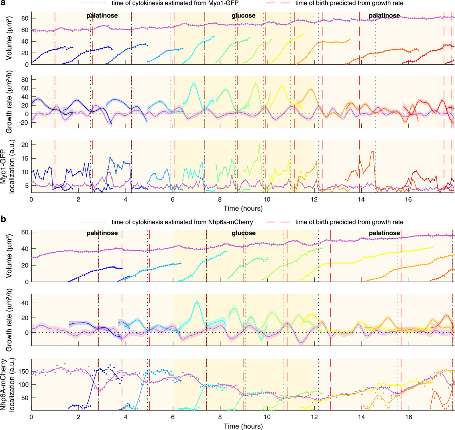
Markers for anaphase and cytokinesis reveal coincidence with a crossing point in mother and bud growth rates.
(a) Time series for a mother (purple) and its buds and daughters for a switch from 2% palatinose to 2% glucose and back, with volumes and growth rates estimated by BABY. We use the localisation of Myo1-GFP to the bud neck to identify times of cytokinesis (vertical black dotted lines). For comparison, we show birth times predicted by our growth rate heuristic as vertical red dashed lines. (b) As for a, but using the localisation of Nhp6A-mCherry to the nucleus to identify times of cytokinesis (vertical black dotted lines). We show both the raw (points) and smoothed (lines; Savitzky-Golay filter with third degree polynomial and smoothing window of 15 time points) localisation of Nhp6A-mCherry.
Tables
Appendix 1—table 1
Optimised post-processing parameters for BABY’s standard model.
The standard model takes five bright-field Z sections with a pixel size of 0.182m as input. Excepting and , we optimised parameters separately for each size category.
| Parameter | |||
|---|---|---|---|
| 0.35 | 0.5 | 0.95 | |
| 0 | 0 | 0 | |
| Connectivity | 2 | 1 | 1 |
| 0 | 0 | 0 | |
| 0 | 0 | 2 | |
| 0.32 | 0.06 | 0.28 | |
| 0.0012 | 0.0028 | 0.0 | |
| 19 | |||
| 0.85 |
Additional files
Download links
A two-part list of links to download the article, or parts of the article, in various formats.
Downloads (link to download the article as PDF)
Open citations (links to open the citations from this article in various online reference manager services)
Cite this article (links to download the citations from this article in formats compatible with various reference manager tools)
Determining growth rates from bright-field images of budding cells through identifying overlaps
eLife 12:e79812.
https://doi.org/10.7554/eLife.79812


