Scale-free behavioral dynamics directly linked with scale-free cortical dynamics
Figures

Simultaneous recording of behavior and neural activity.
(A) Multiplane calcium imaging measured ~10,000 neurons in shallow layers of mouse visual cortex, while a camera measured facial motion and a treadmill measured run speed. (B) Example activity time series from 15 neurons (out of 11,005 total in this recording). Notice some neurons were strongly correlated with behavior (bottom five), while others were anticorrelated (top five), and others were nearly uncorrelated (middle five). (C) The four aspects of behavior - run speed, pupil diameter, speed of changes in gaze direction, and whisker motion - tended to covary on long time scales, but differ in fast fluctuations.
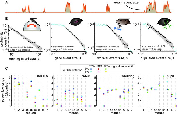
Spontaneous behavior is often scale-free.
(A) Behavioral events (run speed, in this example) are defined by excursions above the median; event size is the area (shaded patch) between the curve and the median. (B) Four examples of behavioral event size distributions with large power-law range r>3 dB. Black points indicate the part of the distribution that is fit well by a power law. Blue points fall outside the power-law range. Gray patch indicates the expected variability (10th to 90th percentile) of the best-fit power law. (C) Summary of power-law range for all mice and all behaviors. Gaze dynamics were least likely to have a large power-law range. All mice had at least one behavior with a very large (>3 decades) power law range. Changes in power-law fitting parameters (goodness-of-fit criteria and outlier criteria) did not change our general conclusions.
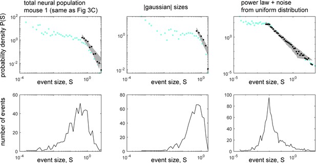
Interpreting probability density functions (PDF) with logarithmic bins.
The best practice for presenting a distribution of a power-law distributed quantity is to use logarithmic bin sizes. However, probability density can be difficult to interpret with logarithmic bins because it represents the count of events in a bin divided by the bin size. Since the bin size can be <<1, the probability density can be high even though the sample counts are low. To make this clear, we show both event counts (bottom row) and PDFs (top row) for three data sets. The left column is from the total population in mouse 1 (same as Figure 3B). The middle column was obtained by drawing sizes from the positive side of a gaussian distribution with the same SD as the data set in the left column (The mean was zero and values less than zero were excluded). Note the similarity of the middle and left columns; both have a poor sampling of small event sizes which manifests as noisy fluctuations in the small size range of the PDF. From this, it appears that the total population is more similar to a truncated gaussian than to a power-law. The right column is a synthetic data set with half the samples drawn from a power-law and half drawn from a uniform distribution on the interval [0, 0.01]. Note the similarity with certain behavioral event size distributions in Figure 2. This suggests that there is a mix of low-amplitude noise and power-law distributed behavioral fluctuations.
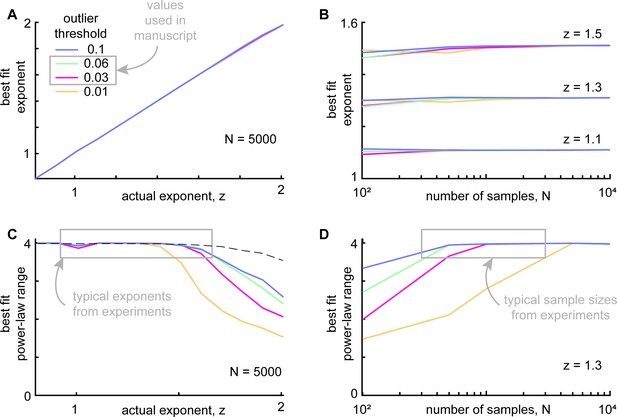
Outlier exclusion effects on power-law fitting algorithm.
In the experimental data, we occasionally found that the distributions of neural or behavioral events had ‘outliers’ – samples that fell far from the distribution, often with a large gap between the outlier point and the nearest neighbor sample. To remove subjective choices from our analysis pipeline we developed a systematic automated algorithm for excluding outliers. Although this outlier exclusion is not subjective, it is still important to understand how it may impact the ability of our power-law fitting algorithm. Here, we benchmarked our outlier exclusion and fitting pipeline on synthetic samples drawn from known power-law distributions. We tested a family of truncated power-law distributions. In all cases, we set the minimum and maximum sample sizes to be 0.01 and 100, respectively. We tested a range of power-law exponents z=0.8 to z=2, where P(s) ~ s-z (like those observed in our experimental results) and sample sizes from N=100 to N=10,000. Finally, we tested outlier cutoff thresholds 0.01, 0.03, 0.06, and 0.1. (A) Our fitting algorithm successfully identified the correct exponent, independent of the outlier threshold (N was fixed at 5000 for all panel A results). (B) Best fit exponents were very slightly underestimated when the sample size was very small, less than about 200. Our typical sample size in the experiments was larger than this. (C) Since excluding outliers inevitably reduces the range of the data, power-law range was more sensitive to outlier threshold, but only for exponents above about 1.7. We note that the neural subsets that were strongly correlated with behavior had much lower exponents (closer to one), for which there is no substantial sensitivity to outlier threshold. Dashed line shows the upper bound on power-law range for N=5000. (D) Power-law range was also underestimated when sample sizes were small. Again, we emphasize for the outlier thresholds we used in our main results (0.03 and 0.06) and the typical sample sizes from the experiments (>400), the best-fit power-law range was not very sensitive to the outlier threshold.
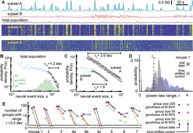
Certain subsets of neurons exhibit scale-free dynamics, but total population does not.
(A) Activity of the total neural population (black) and two subsets of neurons (blue, red) are shown. Each excursion above the median is one neural event (blue shaded area for subset A). Examples in panels A, B, and C are from mouse 1. (B) For the total population, the distribution of neural event sizes is not well fit by a power law (small range rtot = 1.2 decades). Histogram of event sizes (green, same bins used for blue, black distributions) shows that head of the distribution is noisy because very few events had very small sizes. (C) Certain subsets of neurons exhibited very large power-law range (rA = 3.9 decades), while other subsets did not (rB = 1.8 decades). These two example distributions are offset vertically to aid comparison of shape. (D) Distribution of power-law range r for 1000 subsets from mouse 1 (blue). Power law range r reached 4.5 decades for some subsets but did not exceed 2.6 decades for time-shifted controls (gray) in this mouse. (E) Summary of all mice, showing the number of subsets (out of 1000) with power-law range r>3.5 decades, compared to time-shifted controls. Results were qualitatively unchanged for different group size or goodness-of-fit criteria.
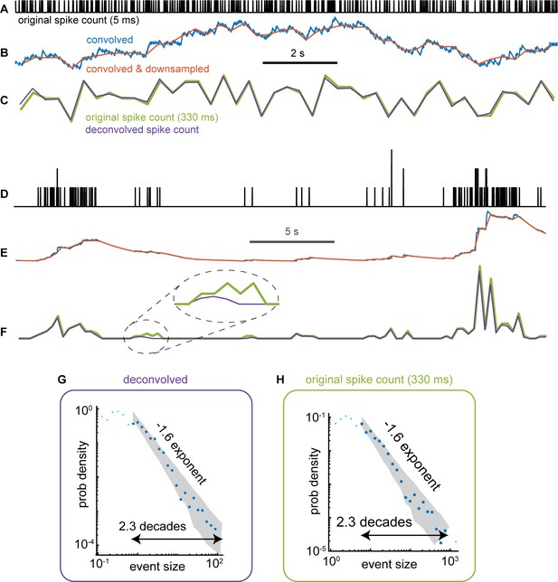
Neural event size distributions are robust to some loss of spikes due to analysis of Ca imaging signals.
Previous studies have shown that the deconvolution used to obtain an estimate of spike rate from raw GCAMP6s Ca signals can result in missing some spikes (Huang et al., 2021). Here, we asked if such missing spikes might distort or bias the event size statistics we report in the main text (Figures 3, 5 and 7). To address this question, we began with time-resolved spike data from 294 single units measured with a Neuropixel probe (the data set was first published by Stringer et al and is labeled Probe 5 from the mouse called Robbins in their online data repository). We first performed a forward-modeling process to create a signal like the GCAMP6s Ca signals we study in our main results. This involved four steps: (1) convolution with a Ca-transient (step increase, exponential decay with 2 s time constant), (2) downsampling to 3 Hz sample rate, (3) non-negative deconvolution with the OASIS algorithm described in Friedrich et al., 2017 and used by Stringer et al., 2019, and (4) z-scoring each neuron’s deconvolved activity time series. We compared the resulting estimate of spike count activity to the ground truth spike count in 330ms time bins. We note that we did not add any noise into these signals, so the results should be considered a best-case scenario. Real experimental measurement tools will, of course, have some noise, which will result in some additional erroneous spikes. (A–F) Two examples of the forward modeling and comparison to ground truth are shown, one example for a high firing rate neuron (panels A-C), another example for a bursty low rate neuron (panels D-F). The dashed line circle in panel F highlights an example where the deconvolution (purple) misses some of the original spikes. (G) Neural event size distribution for the deconvolved 3 Hz data. (H) Neural event size distribution for the ground truth original data, also binned at 3 Hz time resolution. Note that although z-scoring changes the sizes of events, the exponent and range of power-law scaling was nearly unchanged. Thus, we conclude that the spikes missed by deconvolution do not dramatically impact neural event statistics we studied here.
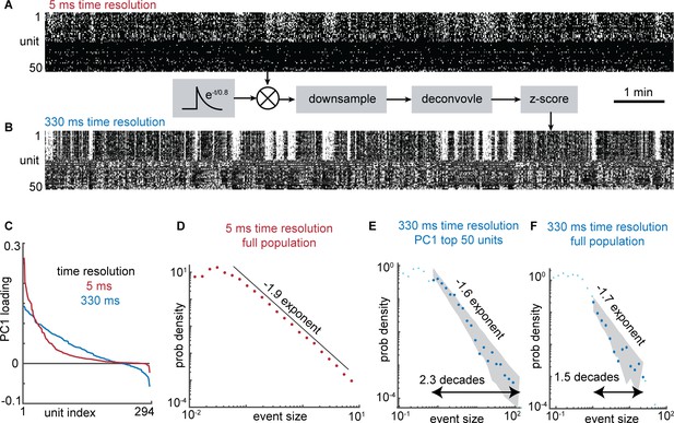
Reconciling fast and slow time scales of electrophysiology and Ca imaging.
Previous studies of scale-free event size distributions have mostly been based on time-resolved electrophysiological data. To better understand how the slow Ca imaging signals we studied here may relate to fast ephys data, we analyzed an example electrophysiological recording of spike times with sub-millisecond time resolution in an awake mouse (data is from a Neuropixel recording in Stringer et al., 2019). (A) First, we examined the data at high time resolution using spike counts in 5ms time bins. Raster shows 50 out of a total of 294 recorded neurons. The first 25 have the largest loadings of the first principal component (PC1). The last 25 have the lowest loadings of PC1. (B) Next, we created a Ca-like signal by convolving the spike times with a Ca-like-transient with a 0.8 s time constant. Then,this signal was downsampled to a 3 Hz sample rate. Then it was deconvolved using the same OASIS nonnegative deconvolution algorithm as was used for the Ca imaging data in our main results. Finally, the signal was z-scored. Raster order is same as panel A, but PC1 was recomputed for the 330 ms resolution data. (C) As is apparent in panel A, the 5ms resolution data exhibited very weak anticorrelations. This was also apparent in the nearly entirely positive loadings of PC1 (red). In contrast, the 330ms resolution data had stronger anticorrelations (about 1/4 of neurons had negative loading in PC1). (D) When considering the entire population of 294 neurons, the 5ms data exhibited a power-law avalanche size distribution with an exponent near –2, consistent with some previous reports of spike avalanches in awake mice (e.g. Ma et al., 2019; Fontenele et al., 2019). (E) When considering the 50 neurons with the largest positive loadings to PC1, the 330 ms resolution data also exhibited power law scaling over a range of 2.3 decades. (F) When the entire population was considered, the 330 ms resolution data exhibited a poorer power law with a relatively short range (1.5 decades) due to cancelation between anticorrelated neurons as discussed in Figure 7 of the main manuscript.
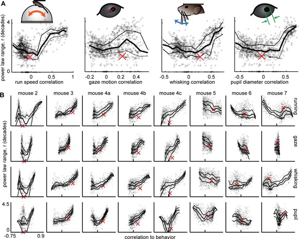
Scale-free neural subsets correlate with behavior, but non-scale-free subsets do not.
(A) Each point represents the power-law range r and behavioral correlation of one neural subset from mouse 1. Subsets with large r tend to be most correlated with behavior. Thick line is a moving average of points; thin lines delineate quartiles. The red x represents the total population. (B) Same as panel A for the other eight recordings. Tick mark on horizontal axis marks zero correlation. Points have partially transparent markers, thus darker areas reveal higher density of points.
Outlier recordings.
Our primary result, shown in Figure 4, was that subset of neurons with large power-law ranges tended to be most strongly correlated to behavior. However, this observation was less pronounced in mouse 5, mouse 6, and mouse 7 recordings (Figure 4). Here, we show that one possible factor that might contribute to the ‘outlier’ tendency for these three recordings is that mice 6 and 7 were much more active. They ran about 50 times more than the next most active animal (mouse 2). Mouse 5 was unusual in that it was the least active animal, moving 10 times less than the next least active animal (mouse 3). It is plausible that these abnormally high or low levels of activity would cause deviations from the main results in Figure 4.
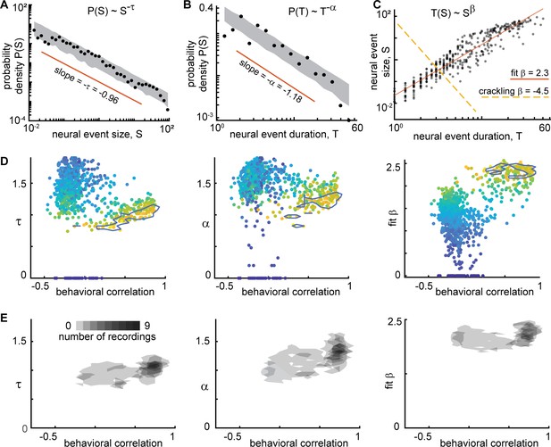
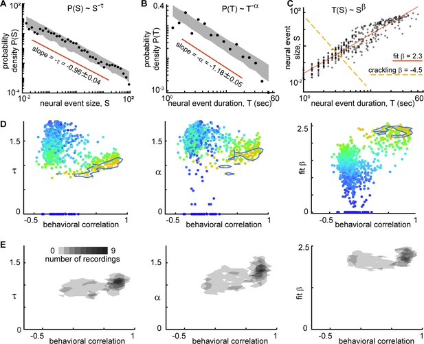
Consistent scaling relations for behaviorally-correlated neural subsets.
(A) Example neural event size distribution with exponent τ=0.96 of the best fit power law (slope on log-log plot). (B) Distribution of event durations with exponent α=1.18 of the best fit power law (same events as in panel A). (C) Event sizes scale with event duration to the power β=2.3. Note that the best fit β is not well predicted by crackling noise theory (gold dashed line). (D) Each point represents one neural subset (color – power law range) from mouse 1. The neural subsets with strongest correlation to behavior (and largest power-law range) exhibited consistent scaling exponents: τ=0.98 ± 0.11, α=1.18 ± 0.19, and fit β=2.18 ± 0.17. Neural subsets with weaker behavioral correlation (smaller power-law range) had widely varying best fit exponents. Contour lines surround points with power-law range >3.5 decades. (E) Summary of all neural subsets with power-law range >3.5 decades from all experiments. Each semi-transparent gray patch corresponds to one contour like the example shown in panel D. The behavioral correlation was chosen to represent the behavior with the greatest correlation for each neural subset.
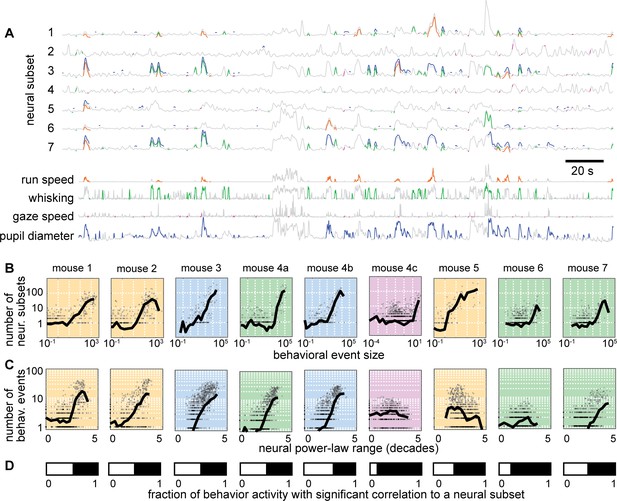
Individual neural events correlate with specific behavioral events.
(A) Time series from 7 example neural subsets and the four behaviors. Each behavioral event with significant correlation to a neural event is indicated with a pair of colored line segments, one on the behavioral time series, one on the neural time series. (B) Behavioral events with greater size were strongly correlated with more neural events (i.e. more neural subsets). (C) Neural subsets with greater power-law range were significantly correlated with a larger number of behavioral events. For panels B and C, each plot summarizes one recording, with one gray point per behavioral event. Black line is a moving average of the points. Background color indicates type of behavior: orange – running; blue – pupil; green – whisking; purple – gaze. (D) The white bar indicates the fraction of behaviorally-active time with strong correlation to a significant number of neural groups. Figure 6—figure supplements 1–2 show similar results for all recordings and behaviors.
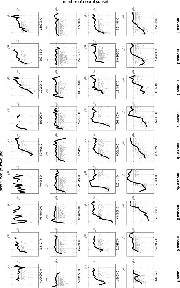
These plots present the same results as Figure 6B, but for all mice and all behaviors.
The left column represents pupil diameter changes, the second column represents gaze dynamics, the third column represents whisking, the right column represents running. The number on the right side of each plot represents the fraction shown in Figure 6D.
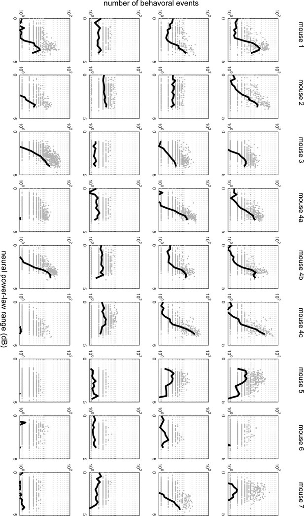
These plots present the same results as Figure 6C, but for all mice and all behaviors.
The left column represents pupil diameter changes, the second column represents gaze dynamics,the third column represents whisking, the right column represents running.
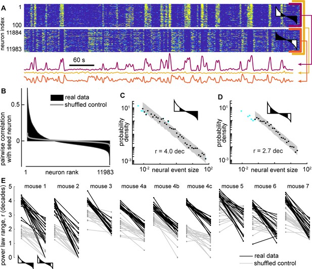
Cancelation of anticorrelated neural subsets hide scale-free neural activity.
(A) Activity of a subset of 100 neurons (top, purple) with large power-law range, another subset of 100 neurons (bottom, orange) that are anticorrelated with first subset, and the total population (yellow). (B) Example correlation spectrum, showing the pairwise correlation coefficients between one seed neuron and all other neurons, ranked in descending order. Gray - control spectrum based on randomly time-shifted neurons. (C) Example neural event size distribution for a subset based on the top 100 most correlated neurons. (D) Example event size distribution for a subset based on the top 50 most correlated neurons and 50 most anticorrelated neurons. Note that the power-law range is greatly reduced compared to panel C. (E) The power-law range for the 50 most correlated (left) is much greater than that of the 50 most extreme (right) neurons. Shown are results for the 20 subsets with the greatest power law range for each mouse. Gray lines represent time-shifted controls, which exhibit smaller power-law range and smaller drop in range due to anticorrelated neurons. In panels A, C, D, and E, the cartoon correlation spectra indicate which neurons were included (white) in subsets and which were not (black).
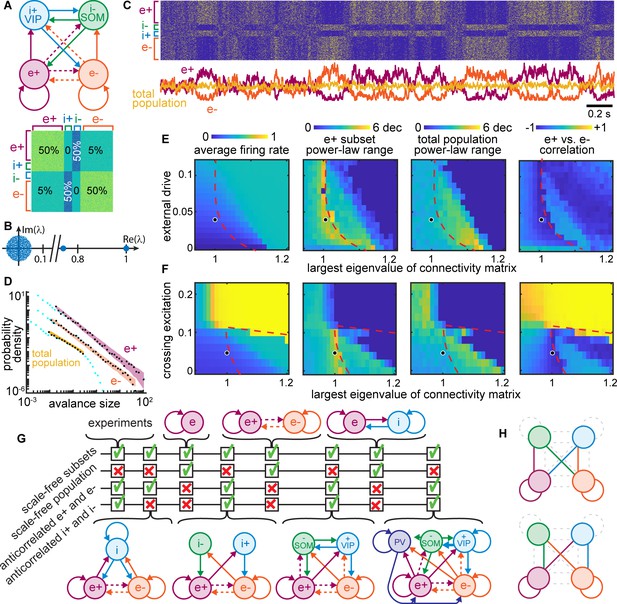
Winner-take-all network structure explains scale-free anticorrelated subsets.
(A) Connectivity diagram (top) and matrix (bottom) illustrate interactions among four populations. Solid, dashed lines indicate dense (50%), sparse (5%) connectivity, respectively. Two excitatory groups (e+ and e−) inhibit each other via dense crossing inhibition. (B) Eigenvalue spectrum of connectivity matrix has two outlying real eigenvalues, the largest equal to 1. (C) Timeseries and raster reveal strong anti-correlations between e+ and e− populations which cancel out; total population has small fluctuations. (D) Neural event distributions for e+ and e− exhibit large power-law range, while the total population does not. (E) Parameter space for model. Model agrees with experiments near dashed line for a wide range of input rates, most with largest eigenvalue is near 1. (F) Dense crossing excitation from e+ to e− abolishes winner-take-all dynamics. (G) Crossing inhibition motif is important for matching our experimental observations. Realistic topologies, including known connectivity among PV+, VIP, and SOM inhibitory neurons (right), contain this crossing inhibition motif and match our observations, but simpler networks can match as well. (H) Considering 8,73,000 different network configurations, only 31 match our experimental observations. All matching configurations had one of these two motifs. Dashed lines indicate unnecessary connections. Figure 8—figure supplement 1 shows all matching configurations.
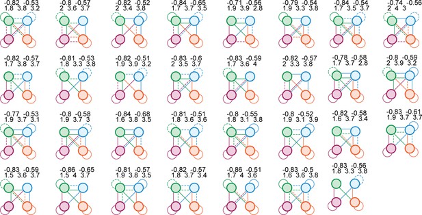
We tried 8,73,000 different network configurations.
Here, we show the 31 configurations that successfully reproduced our primary experimental results. The color scheme and meaning of solid and dashed lines are the same as in Figure 8. The numbers above each circuit diagram report the correlation coefficient between e+ and e− (top left), the correlation coefficient between i+ and i− (top right), power-law range for the total population (bottom left), power-law range for e+ (bottom middle), and power-law range for e− (bottom right).
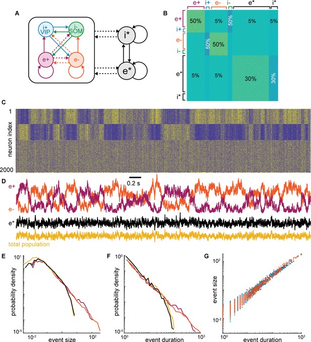
Model with asynchronous population.
Building upon the model presented in Figure 8A–F, we added a population of 1000 more neurons (e* and i*) that has uniform connectivity density to the original model population (e+, i+, e−, i−). Also, the value of each non-zero connection weight was drawn from a uniform distribution [0,0.01] or [–0.01,0] for excitatory and inhibitory connections, respectively. This non-uniform connection strength shows that the uniform connections in Figure 8A–F are not important for the model dynamics. The new group (e*) exhibits asynchronous firing because it gets approximately equal input from both the e+ and e− groups. Thus the large power-law fluctuations of each e+ and e− cancel out resulting in a relatively steady level of input to e* and, thus, no power-law fluctuations in e*. (A) Schematic of connectivity among groups. (B) Color visualization of the entire 2000 × 2000 connectivity matrix for all neurons. Different colors indicate density of connectivity (also marked as percentages) and whether connections are excitatory (yellow) or inhibitory (blue). (C) Example spike raster from the model with rows ordered in the same way as the rows of the connectivity matrix in panel B. (D) Population average activity time series for e+ and e− have large amplitude anticorrelated fluctuations just like the original model in Figure 8A–F. The activity of e* (black) has small fluctuations like the total population (gold). (E–G) The fluctuations of e+ and e− have power-law distributed event sizes and durations as well as size versus duration scaling. The total population and e* are not power-law distributed. These distributions were generated from 1,00,000-time steps of the simulation (much longer than the example time series in panels C and D).
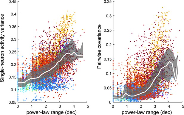
Single-neuron variance and pairwise covariance are larger for neural subsets with large power-law range.
(left) Each point represents one subset of neurons from the experiments. For each subset, the activity variance was computed for each neuron and then averaged over neurons. Subsets with large single-neuron variance tended to have large power-law range. (right) Each point represents the average pairwise covariance of all neurons within a subset. Subsets with large covariance tended to have large power-law range. White line is the median of points, gray band delineates quartiles. Color of points indicates recording (mouse 1 – red, mouse 2 – dark blue, mouse 3 – gold, mouse 4 a – purple, mouse 4b – green, mouse 4 c – cyan, mouse 5 – dark red, mouse 6 – blue, mouse 7 – orange).
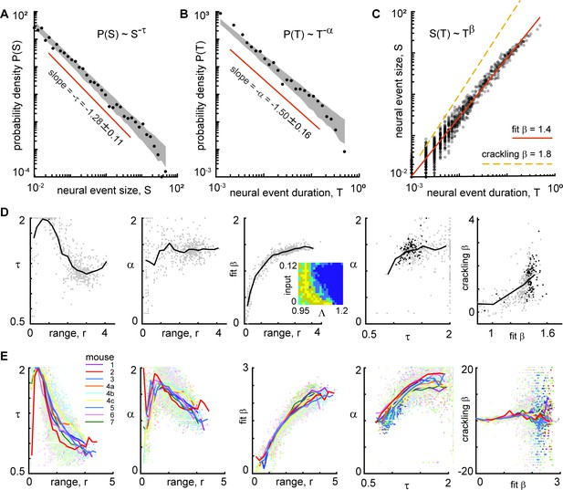
Consistent scaling laws for large power-law range in model and experiment.
(A) Model example neural event size distribution with exponent τ=1.28 of the best fit power law. (B) Distribution of event durations from model with exponent α=1.5. (C) Event sizes scale with event duration to the power β=1.4. Note that the best-fit β is not well predicted by crackling noise theory (gold dashed line). (D) For the model, best fit scaling exponents τ, α, and β are consistent for large power-law range, but not for low power law range. Each gray point represents one run of the model. Different points come from different parameters (input and Λ) with non-zero power-law range. Inset in middle shows how many points came from each parameter combination (yellow = 4, dark blue = 0). Black points in right panels represent model parameters with power-law range above three decades. (E) Same as panel D, but experimental data are shown. Each point represents one neural subset. Color represents mouse. Experiment and model follow similar trends, but experiments tended to have smaller τ and larger β than the model, for large r. Crackling noise predictions of β are poor for both experiment and model. Dark colored points in right panels represent neural subsets with power-law range above 3.5 decades.
Tables
| Reagent type (species) or resource | Designation | Source or reference | Identifiers | Additional information |
|---|---|---|---|---|
| Software,algorithm | Matlab | Mathworks | R2018a |


