Figures and data in Sparse dimensionality reduction approaches in Mendelian randomisation with highly correlated exposures

Version of Record

Accepted for publication after peer review and revision.

Download
Cite
Share
CommentOpen annotations (there are currently 0 annotations on this page).

Version of Record published: May 30, 2023 (This version)
Accepted Manuscript published: April 19, 2023 (Go to version)
Accepted: April 18, 2023
Preprint posted: June 16, 2022 (Go to version)
Received: May 6, 2022

Figures
Tables
Additional files

19 figures, 7 tables and 1 additional file

Figures

Figure 1

Download asset Open asset

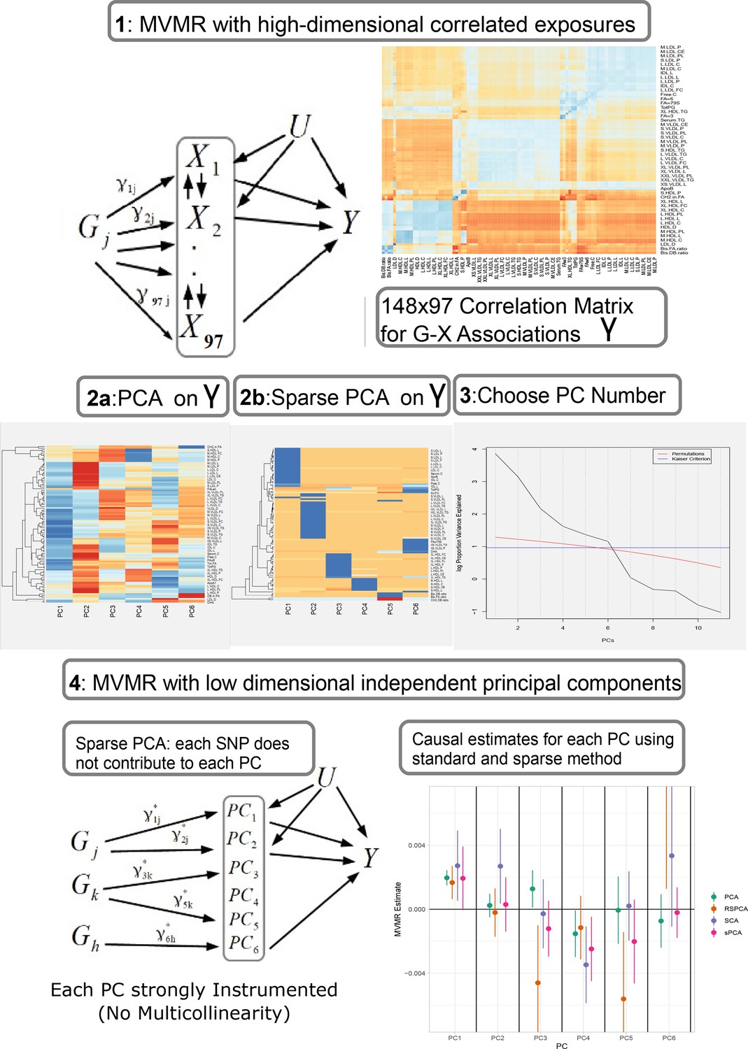
Proposed workflow.

Step 1: MVMR on a set of highly correlated exposures. Each genetic variant contributes to each exposure. The high correlation is visualised in the similarity of the single-nucleotide polymorphism (SNP)-exposure associations in the correlation heatmap (top right). Steps 2 and 3: PCA and sparse PCA on $\hat{γ}$ . Step 4. MVMR analysis on a low dimensional set of principal components (PCs). X: exposures; Y: outcome; k: number of exposures; PCA: principal component analysis; MVMR: multivariable Mendelian randomisation.

Figure 2

Download asset Open asset

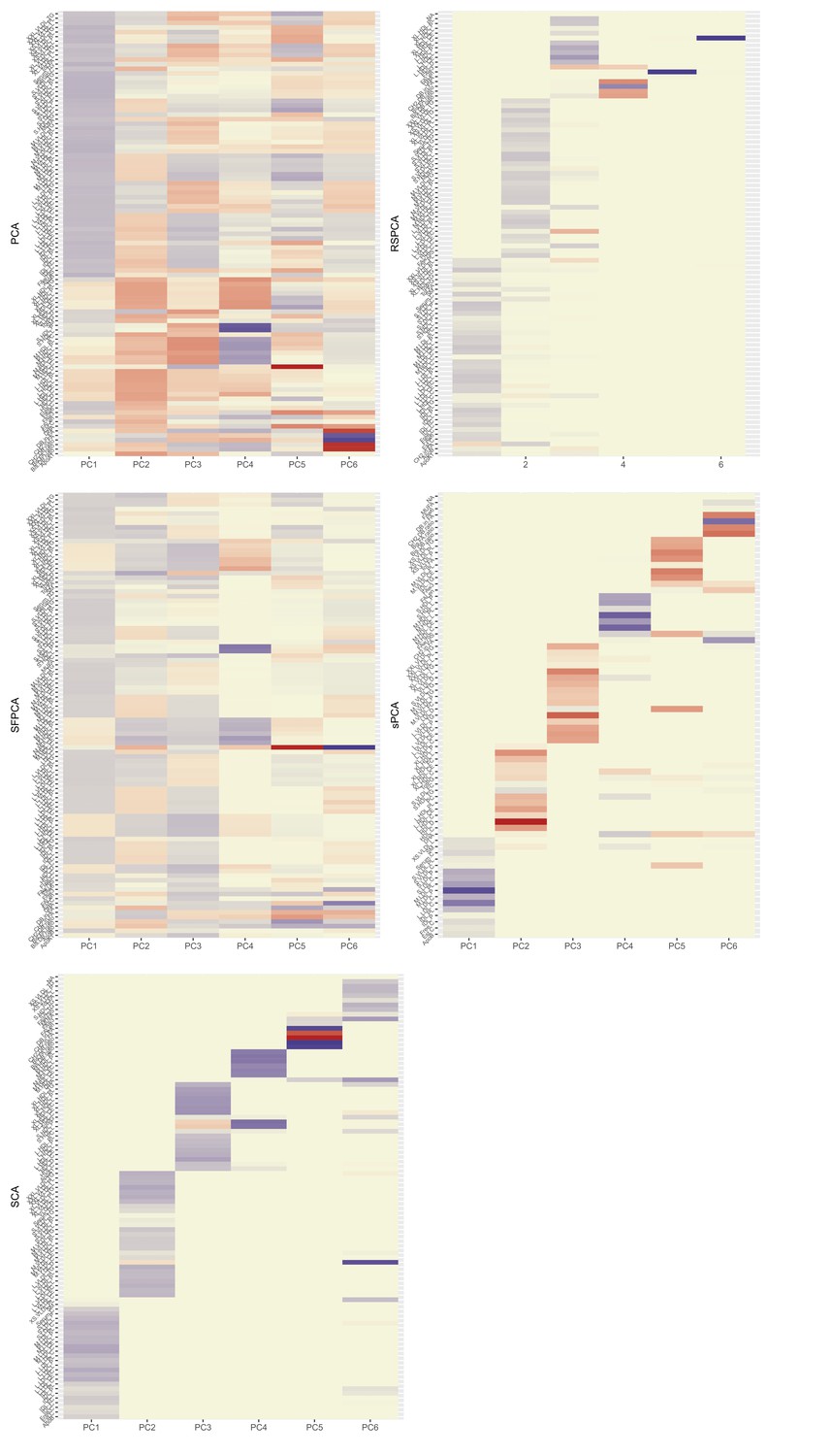
Heatmaps for the loadings matrices in the Kettunen dataset for all methods (one with no sparsity constraints [a], four with sparsity constraints under different assumptions [**b–e**]).

The number of the exposures plotted on the vertical axis is smaller than $K = 97$ as the exposures that do not contribute to any of the sparse principal components (PCs) have been left out. Blue: positive loading; red: negative loading; yellow: zero.

Figure 3

Download asset Open asset

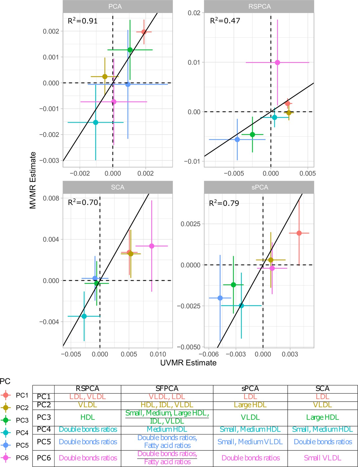
Comparison of univariable Mendelian randomisation (UVMR) and multivariable MR (MVMR) estimates and presentation of the major group represented in each principal component (PC) per method.

Figure 4

Download asset Open asset

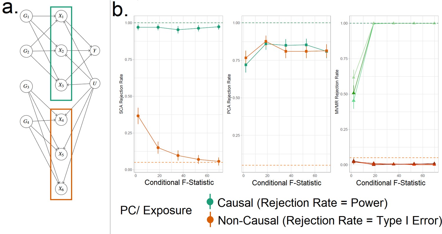
Simulation Study Outline.

(a) Data generating mechanism for the simulation study, illustrative scenario with six exposures and two blocks. In red boxes, the exposures that are correlated due to a shared genetic component are highlighted. (b) Simulation results for six exposures and three methods (sparse component analysis [SCA] [Chen and Rohe, 2021], principal component analysis [PCA], multivariable Mendelian randomisation [MVMR]). The exposures that contribute to $Y$ ( $X_{1 - 3}$ ) are presented in shades of green colour and those that do not in shades of red ( $X_{4 - 6}$ ). In the third panel, each exposure is a line. In the first and second panels, the PCs that correspond to these exposures are presented *as single lines* in green and red. Monte Carlo SEs are visualised as error bars. Rejection rate: proportion of simulations where the null is rejected.

Figure 5

Download asset Open asset

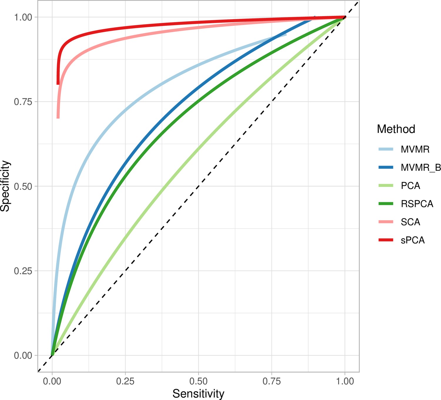
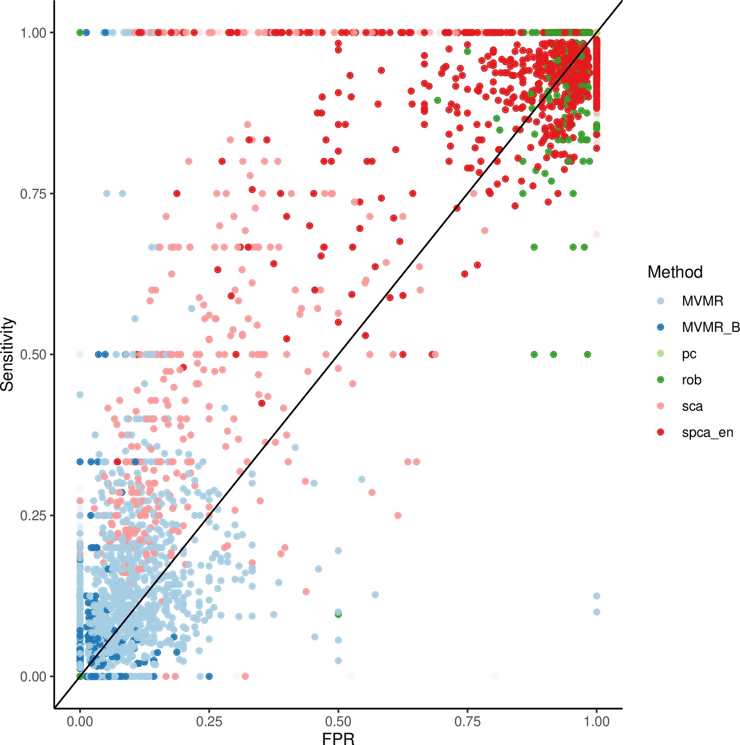
Extrapolated receiver-operating characteristic (ROC) curves for all methods.

SCA: sparse component analysis (Chen and Rohe, 2021) sPCA: sparse PCA (Zou et al., 2006) RSPCA: robust sparse PCA (Croux et al., 2013); PCA: principal component analysis; MVMR: multivariable Mendelian randomisation; MVMR_B: MVMR with Bonferroni correction.

Figure 6

Download asset Open asset

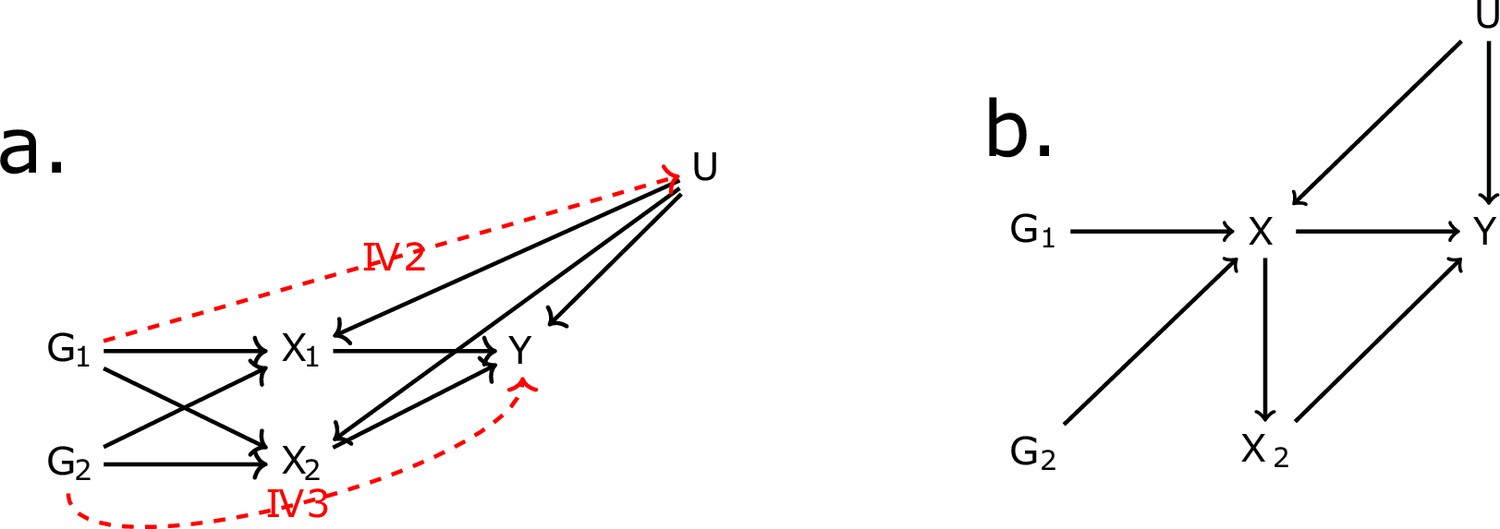
Directed acyclic graph (DAG) for the multivariable Mendelian randomisation (MVMR) assumptions.

IV2, IV3: instrumental variable assumptions 2 and 3.

Appendix 1—figure 1

Download asset Open asset

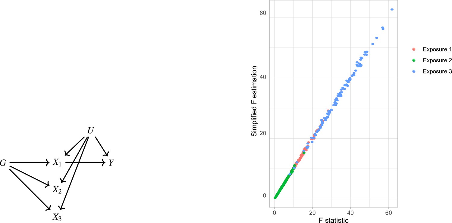
Simplified F-statistic Estimation.

(a) Data generating mechanism. Three exposures with different degrees of strength of association with $G$ are generated $γ_{1} = 1, γ_{2} = 0.5, γ_{3} = 0.1$ . (b) $F$ -statistic for the three exposures $X_{1}, X_{2}, X_{3}$ as estimated by the formulae in Equation 5 (horizontal axis) and Equation 4 (vertical axis).

Appendix 1—figure 2

Download asset Open asset

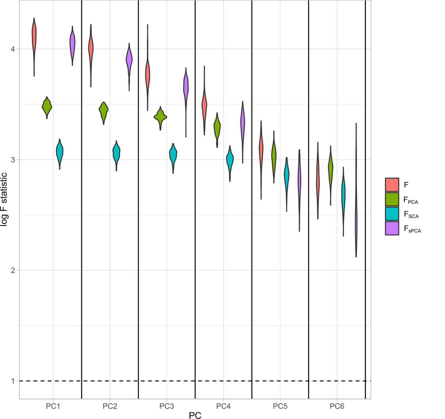
Distributions of the F-statistics in principal component analysis (PCA) methods and individual (not transformed) exposures.

Exposure data in different blocks are simulated with a decreasing strength of association and the correlated blocks map to principal components (PCs). Each distribution represents the F-statistics for each PC. In the case of the individual exposures (red), the distributions represent the F-statistics for the corresponding exposures. Individual: individual exposures without any transformation; PCA: F-statistics for PCA; SCA: sparse component analysis (Chen and Rohe, 2021) sPCA: sparse PCA as described by Zou et al., 2006.

Appendix 1—figure 3

Download asset Open asset

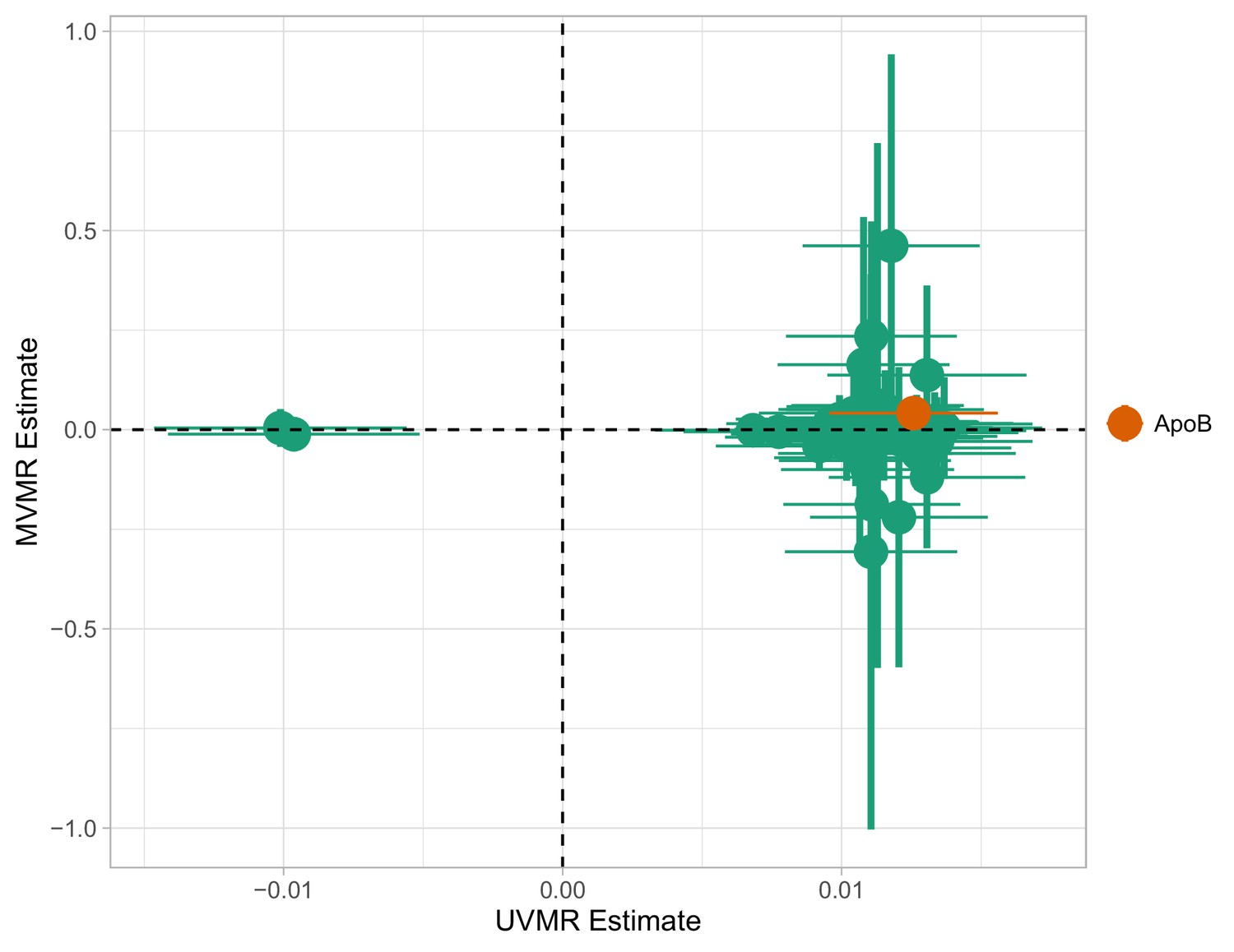
Multivariable Mendelian randomisation (MVMR) and univariable MR (UVMR) estimates.

Only ApoB is strongly associated with coronary heart disease (CHD). All SEs are larger in the MVMR model (range of $\frac{S E_{M V M R}}{S E_{U V M R}} 2.7 - 225.96$ ).

Appendix 1—figure 4

Download asset Open asset

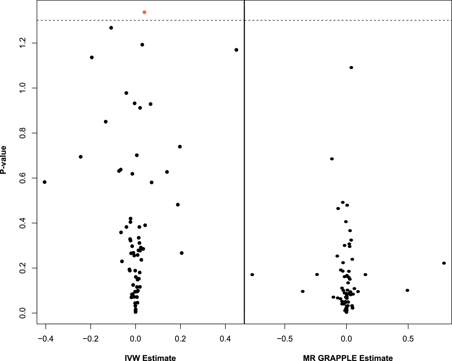
Multivariable Mendelian randomisation (MVMR) with IVW (left) and MVMR with GRAPPLE (Zhao et al., 2021) (right).

Only the 66 exposures. that are significant in univariable MR (UVMR) are put forward in these models. In IVW (left), ApoB shows nominal significance. In MR GRAPPLE (right), apolipoprotein B has the lowest p-value but no trait reaches nominal significance.

Appendix 1—figure 5

Download asset Open asset

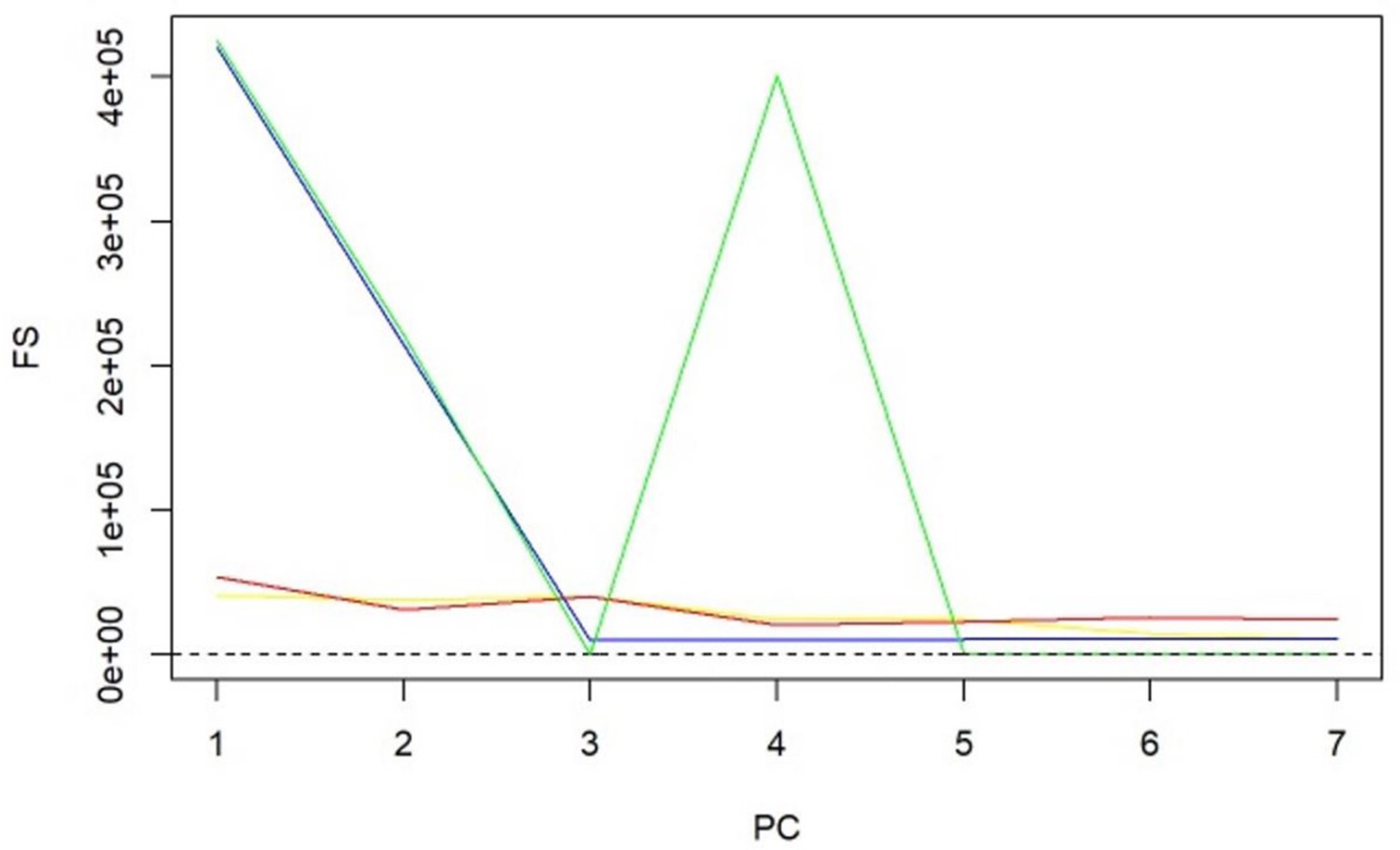
$F$ -statistics for principal components (PCs) and sparse PCs.

The formula derived in Equation 5 is used. Black: principal component analysis (PCA) (no sparsity constraints); yellow: sparse component analysis (SCA); red: sparse PCA (Zou); blue: sparse robust PCA; green: sparse fused PCA. The dashed line represents the cutoff of 10 that is considered the minimum desired $F$ -statistic for an exposure to be considered well instrumented. The green line diverges from the pattern of decreasing instrument strength but, when referring to the loadings heatmap (Figure 2), it can be observed that the 4th sparse PC in the fused sPCA receives negative loadings from multiple very low-density lipoprotein (VLDL)- and low-density lipoprotein (LDL)-related traits. This may in turn cause the large $F$ -statistic.

Appendix 1—figure 6

Download asset Open asset

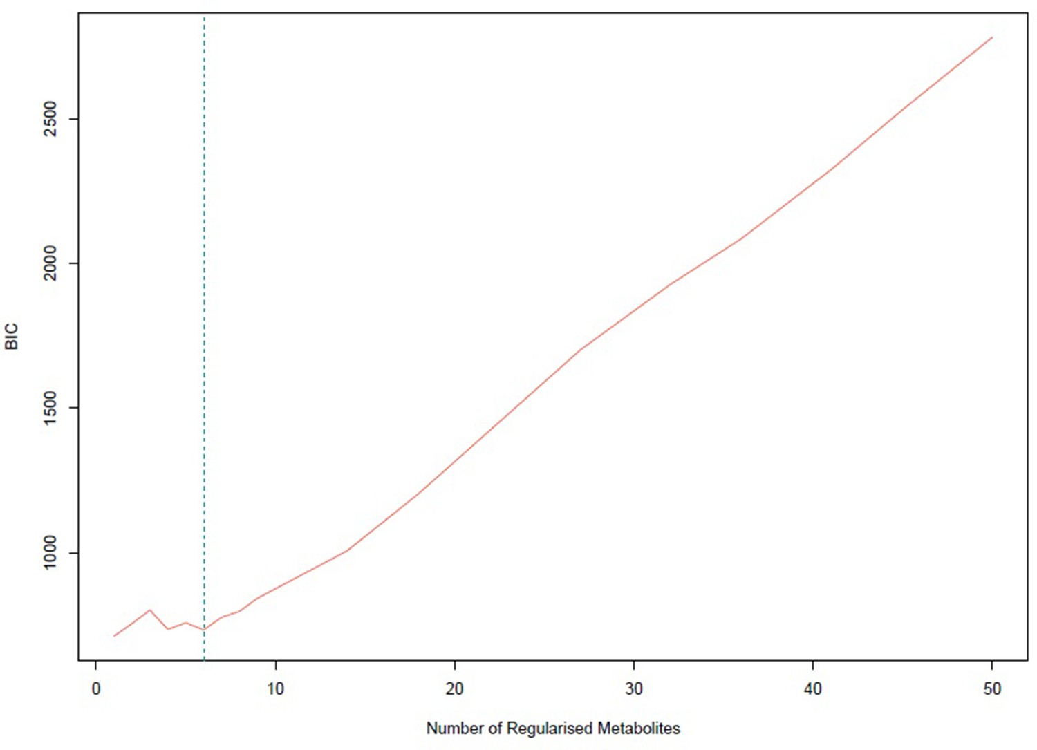
Bayesian information criterion (BIC) for different numbers of metabolites regularized to 0.

The lowest value is achieved for one non-zero exposure per component. However, six non-zero exposures per component also achieved a similar low BIC and this was selected.

Appendix 1—figure 7

Download asset Open asset

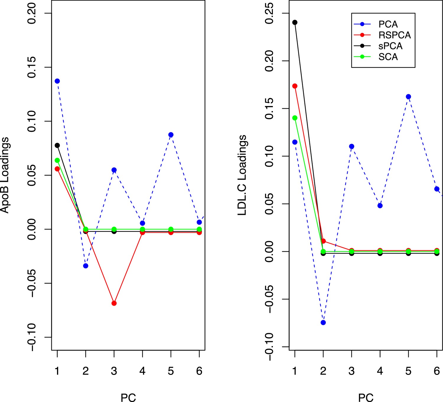
Trajectories for the loadings of total cholesterol in low-density lipoprotein (LDL) and ApoB in all methods.

Principal component analysis (PCA) loadings imply a contribution of LDL.c and ApoB to all principal components (PCs). In the sparse methods, this is limited to one PC (two for RSPCA).

Appendix 1—figure 8

Download asset Open asset

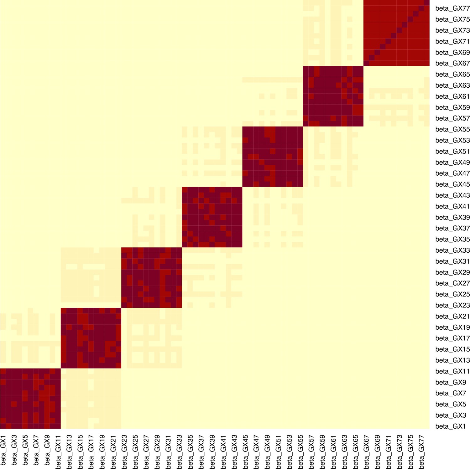
Example for the block correlation in $\hat{γ}$ ( $n = 5000$ , $K = 77$ ) induced by the data generating mechanism in Figure 4.

In this example, the mean $F$ -statistic is 231.2 and the mean $C F S$ is 3.21.

Appendix 1—figure 9

Download asset Open asset

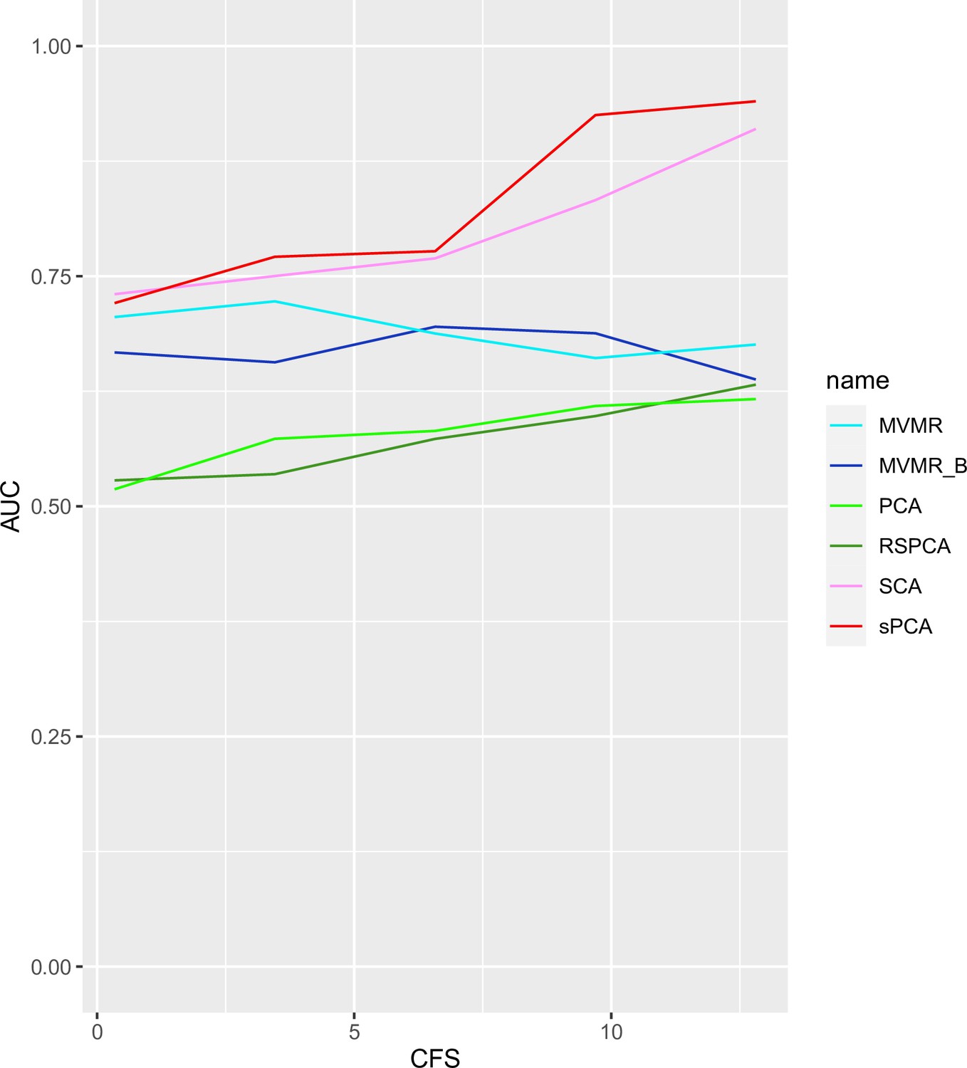
AUC performance of multivariable Mendelian randomisation (MVMR) and dimensionality reduction methods for increasing sample sizes.

Two sparse methods (sparse component analysis [SCA], sparse principal component analysis [sPCA]) perform better compared with PCA and MVMR, with improving performance as the sample size increases. CFS: conditional F-statistic.

Appendix 1—figure 10

Download asset Open asset

Individual results from $s = 1000$ simulations.

Appendix 1—figure 11

Download asset Open asset

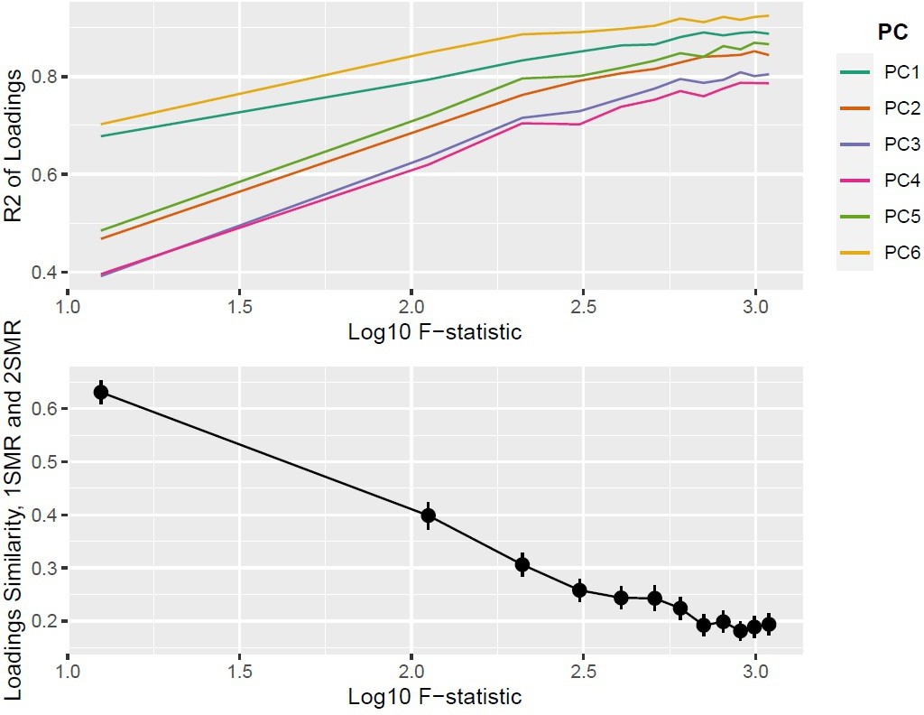
Top panel: $R^{2}$ ; bottom panel: similarity of loadings ( $S$ ) between one-sample Mendelian randomisation (MR) and two-sample MR ( $N_{s i m} = 10, 000$ ).

Appendix 1—figure 12

Download asset Open asset

Specificity (ability to accurately identify true negative exposures) of sparse component analysis (SCA) as a different proportion of exposures in each block are causal for $Y$ .

Author response image 1

Download asset Open asset

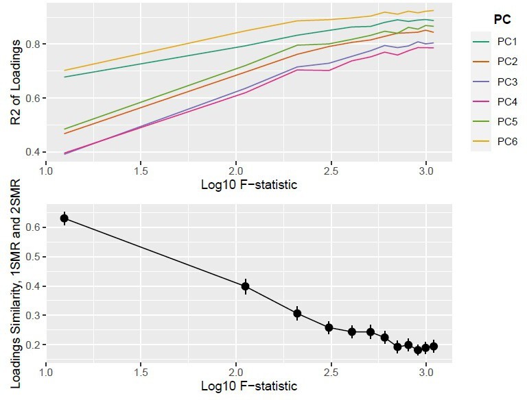
Top Panel: R²; Bottom Panel: Similarity of loadings (*S_load*) between one-sample MR and two-sample MR (*N_sim* = 10,000).

Tables

Table 1

Univariable Mendelian randomisation (MR) results for the Kettunen dataset with coronary heart disease (CHD) as the outcome.

Positive: positive causal effect on CHD risk; Negative: negative causal effect on CHD risk.

	Positive	Negative
VLDL	AM.VLDL.C, M.VLDL.CE, M.VLDL.FC, M.VLDL.L,M.VLDL.P, M.VLDL.PL, M.VLDL.TG, XL.VLDL.L,XL.VLDL.PL, XL.VLDL.TG, XS.VLDL.L, XS.VLDL.P, XS.VLDL.PL,XS.VLDL.TG, XXL.VLDL.L, XXL.VLDL.PL,L.VLDL.C, L.VLDL.CE, L.VLDL.FC, L.VLDL.L, L.VLDL.P,L.VLDL.PL, L.VLDL.TG, SVLDL.C, S.VLDL.FC,S.VLDL.L, S.VLDL.P, S.VLDL.PL, S.VLDL.TG	None
LDL	ALDL.C, L.LDL.C, L.LDL.CE, L.LDL.FC, L.LDL.L, L.LDL.P, L.LDL.PL,M.LDL.C, M.LDL.CE, M.LDL.L, M.LDL.P,M.LDL.PL, S.LDL.C, S.LDL.L, S.LDL.P	None
HDL	S.HDL.TG, XL.HDL.TG	M.HDL.C, M.HDL.CE

Table 2

Overview of sparse principal component analysis (sPCA) methods used.

KSS: Karlis-Saporta-Spinaki criterion. Package: R package implementation; Features: short description of the method; Choice: method of selection of the number of informative components in real data; PCs: number of informative PCs.

Method	Package	Authors	Features	Choice	PCs
RSPCA	pcaPP	Croux et al., 2013	Robust sPCA (RSPCA), different measure of dispersion ( $Q_{n}$ )	Permutation KSS	6
SFPCA	Code in publication, Supplementary Material	Guo et al., 2010	Fused penalties for block correlation	KSS	6
sPCA	elasticnet	Zou et al., 2006	Formulation of sPCA as a regression problem	KSS	6
SCA	SCA	Chen and Rohe, 2021	Rotation of eigen vectors for approximate sparsity	Permutation KSS	6

Table 3

Results for principal component analysis (PCA) approaches.

Overlap: Percentage of metabolites receiving non-zero loadings in ≥1 component. Overlap in PC1, PC2: overlap as above but exclusively for the first two components which by definition explain the largest proportion of variance. Very low-density lipoprotein (VLDL), low-density lipoprotein (LDL), and high-density lipoprotein (HDL) significance: results of the IVW regression model with CHD as the outcome for the respective sPCs (the sPCs that mostly received loadings from these groups). The terms VLDL and LDL refer to the respective transformed blocks of correlated exposures; for instance, VLDL refers to the weighted sum of the correlated VLDL-related $\hat{γ}$ associations, such as VLDL phospholipid content and VLDL triglyceride content. †: RSPCA projected VLDL- and LDL-related traits to the same PC (sPC1). ‡: SCA discriminated HDL molecules in two sPCs, one for traits of small- and medium-sized molecules and one for large- and extra-large-sized.

	PCA	RSPCA	SFPCA	sPCA	SCA
Overlap	1	0.938	1	0.187	0.196
Overlap in PC1,PC2	1	0.433	1	0.010	0
Sparse %	0	0.474	0.082	0.835	0.796
VLDL significance in MR†	Yes	No	Yes	No	Yes
LDL significance in MR	No	Yes	No	No	Yes
HDL significance in MR‡	Yes	Yes	Yes	No	No
Small, medium HDL significance in MR	Yes	No	Yes	Yes	Yes

Table 4

Sensitivity and specificity presented as median and interquartile range across all simulations.

Presented as median sensitivity/specificity and interquartile range across all simulations; AUC: area under the receiver-operating characteristic (ROC) curve.

	PCA	SCA	sPCA	RSPCA	MVMR_B	MVMR
AUC	0.56	0.919	0.941	0.644	0.660	0.712
Sensitivity	1,0.1	1,0.21	1, 0.047	0.667, 0.251	0.222, 0.2	0, 0.076
Specificity	0,0.02	0.925,0.772	0.936, 0.097	0.192, 0.104	0.960, 0.048	1,0
Youden’s J	0	0.584	0.778	–0.061	0.192	0.044

Table 5

Two-sample Mendelian randomisation (MR).

Study characteristics.

	First author	Year	PMID	N	Cases	Controls	Study name (population)
Metabolites	Kettunen	2016	27005778	24,925			NMR GWAS (European)
CHD	Nelson	2017	28714975	453,595	113,937	339,658	CARDIoGRAMplusC4D (European)

Appendix 1—table 1

Estimated causal effects of principal components (PCs) on coronary heart disease (CHD) risk.

PCA: principal component analysis; SCA: sparse component analysis; sPCA: sparse PCA (Zou et al., 2006); RSPCA: robust sparse PCA.

PC	Method	OR	LCI	UCI
PC1	PCA	1.002	1.0015	1.0024
PC2	PCA	1.0002	0.9995	1.001
PC3	PCA	1.0013	1.0001	1.0024
PC4	PCA	0.9985	0.997	0.9999
PC5	PCA	0.9999	0.9978	1.002
PC6	PCA	0.9993	0.9976	1.0009
PC1	SCA	1.0027	1.0005	1.0049
PC2	SCA	1.0027	1.0004	1.005
PC3	SCA	0.9997	0.9976	1.0019
PC4	SCA	0.9965	0.9941	0.9989
PC5	SCA	1.0002	0.998	1.0024
PC6	SCA	1.0034	0.9989	1.0078
PC1	sPCA	1.0019	0.9999	1.0039
PC2	sPCA	1.0003	0.9986	1.002
PC3	sPCA	0.9988	0.997	1.0005
PC4	sPCA	0.9975	0.9955	0.9995
PC5	sPCA	0.998	0.9954	1.0006
PC6	sPCA	0.9998	0.9982	1.0014
PC1	RSPCA	1.0017	1.0006	1.0027
PC2	RSPCA	0.9998	0.9983	1.0013
PC3	RSPCA	0.9954	0.9918	0.999
PC4	RSPCA	0.9989	0.9969	1.0008
PC5	RSPCA	0.9944	0.9903	0.9986
PC6	RSPCA	1.01	1.0013	1.0188
PC1	SFPCA	1.002	1.0015	1.0025
PC2	SFPCA	0.9991	0.9979	1.0004
PC3	SFPCA	0.9998	0.9991	1.0006
PC4	SFPCA	0.9982	0.9967	0.9997
PC5	SFPCA	1.0001	0.9977	1.0025
PC6	SFPCA	1.0009	0.9985	1.0033

Appendix 1—table 2

Simulation study on only four exposures (out of the total $K = 50$ ) contributing to the outcome $Y$ .

A drop in sensitivity and specificity is observed for sparse component analysis (SCA) and sparse principal component analysis (sPCA) compared with the simulation configuration in Table 4.

	PCA	SCA	sPCA	RSPCA	MVMR	MVMR_B
AUC	0.799	0.714	0.859	0.492	0.511	0.675
SNS	1,0.03	0.75,0.25	1,0.17	0.5,0.25	0.25,0.25	0,0
SPC	0,0.2	0.76,0.46	0.66,0.18	0.37,0.15	0.94,0.07	1,0
Youden’s J	0	0.428	0.625	–0.029	0.105	0.032

Additional files

MDAR checklist: https://cdn.elifesciences.org/articles/80063/elife-80063-mdarchecklist1-v2.docx
Download elife-80063-mdarchecklist1-v2.docx

Download links

A two-part list of links to download the article, or parts of the article, in various formats.

Downloads (link to download the article as PDF)

Article PDF

Open citations (links to open the citations from this article in various online reference manager services)

Mendeley

Cite this article (links to download the citations from this article in formats compatible with various reference manager tools)

Vasileios Karageorgiou
Dipender Gill
Jack Bowden
Verena Zuber

(2023)

Sparse dimensionality reduction approaches in Mendelian randomisation with highly correlated exposures

eLife 12:e80063.

https://doi.org/10.7554/eLife.80063

Figures

Proposed workflow.

Heatmaps for the loadings matrices in the Kettunen dataset for all methods (one with no sparsity constraints [a], four with sparsity constraints under different assumptions [b–e]).

Comparison of univariable Mendelian randomisation (UVMR) and multivariable MR (MVMR) estimates and presentation of the major group represented in each principal component (PC) per method.

Simulation Study Outline.

Extrapolated receiver-operating characteristic (ROC) curves for all methods.

Directed acyclic graph (DAG) for the multivariable Mendelian randomisation (MVMR) assumptions.

Simplified F-statistic Estimation.

Distributions of the F-statistics in principal component analysis (PCA) methods and individual (not transformed) exposures.

Multivariable Mendelian randomisation (MVMR) and univariable MR (UVMR) estimates.

Multivariable Mendelian randomisation (MVMR) with IVW (left) and MVMR with GRAPPLE (Zhao et al., 2021) (right).

$F$ -statistics for principal components (PCs) and sparse PCs.

Bayesian information criterion (BIC) for different numbers of metabolites regularized to 0.

Trajectories for the loadings of total cholesterol in low-density lipoprotein (LDL) and ApoB in all methods.

Example for the block correlation in $\hat{γ}$ ( $n = 5000$ , $K = 77$ ) induced by the data generating mechanism in Figure 4.

AUC performance of multivariable Mendelian randomisation (MVMR) and dimensionality reduction methods for increasing sample sizes.

Individual results from $s = 1000$ simulations.

Top panel: $R^{2}$ ; bottom panel: similarity of loadings ( $S$ ) between one-sample Mendelian randomisation (MR) and two-sample MR ( $N_{s i m} = 10, 000$ ).

Specificity (ability to accurately identify true negative exposures) of sparse component analysis (SCA) as a different proportion of exposures in each block are causal for $Y$ .

Top Panel: R²; Bottom Panel: Similarity of loadings (S_load) between one-sample MR and two-sample MR (N_sim = 10,000).

Tables

Univariable Mendelian randomisation (MR) results for the Kettunen dataset with coronary heart disease (CHD) as the outcome.

Overview of sparse principal component analysis (sPCA) methods used.

Results for principal component analysis (PCA) approaches.

Sensitivity and specificity presented as median and interquartile range across all simulations.

Two-sample Mendelian randomisation (MR).

Estimated causal effects of principal components (PCs) on coronary heart disease (CHD) risk.

Simulation study on only four exposures (out of the total $K = 50$ ) contributing to the outcome $Y$ .

Additional files

MDAR checklist

Download links

Downloads (link to download the article as PDF)

Open citations (links to open the citations from this article in various online reference manager services)

Cite this article (links to download the citations from this article in formats compatible with various reference manager tools)

Be the first to read new articles from eLife

Share this article

Cite this article

Proposed workflow.

Heatmaps for the loadings matrices in the Kettunen dataset for all methods (one with no sparsity constraints [a], four with sparsity constraints under different assumptions [b–e]).

Comparison of univariable Mendelian randomisation (UVMR) and multivariable MR (MVMR) estimates and presentation of the major group represented in each principal component (PC) per method.

Simulation Study Outline.

Extrapolated receiver-operating characteristic (ROC) curves for all methods.

Directed acyclic graph (DAG) for the multivariable Mendelian randomisation (MVMR) assumptions.

Simplified F-statistic Estimation.

Distributions of the F-statistics in principal component analysis (PCA) methods and individual (not transformed) exposures.

Multivariable Mendelian randomisation (MVMR) and univariable MR (UVMR) estimates.

Multivariable Mendelian randomisation (MVMR) with IVW (left) and MVMR with GRAPPLE (Zhao et al., 2021) (right).

F-statistics for principal components (PCs) and sparse PCs.

Bayesian information criterion (BIC) for different numbers of metabolites regularized to 0.

Trajectories for the loadings of total cholesterol in low-density lipoprotein (LDL) and ApoB in all methods.

Example for the block correlation in γ^ (n=5000, K=77) induced by the data generating mechanism in Figure 4.

AUC performance of multivariable Mendelian randomisation (MVMR) and dimensionality reduction methods for increasing sample sizes.

Individual results from s=1000 simulations.

Top panel: R2; bottom panel: similarity of loadings (S) between one-sample Mendelian randomisation (MR) and two-sample MR (Ns⁢i⁢m=10,000).

Specificity (ability to accurately identify true negative exposures) of sparse component analysis (SCA) as a different proportion of exposures in each block are causal for Y.

Top Panel: R2; Bottom Panel: Similarity of loadings (Sload) between one-sample MR and two-sample MR (Nsim = 10,000).

Univariable Mendelian randomisation (MR) results for the Kettunen dataset with coronary heart disease (CHD) as the outcome.

Overview of sparse principal component analysis (sPCA) methods used.

Results for principal component analysis (PCA) approaches.

Sensitivity and specificity presented as median and interquartile range across all simulations.

Two-sample Mendelian randomisation (MR).

Estimated causal effects of principal components (PCs) on coronary heart disease (CHD) risk.

Simulation study on only four exposures (out of the total K=50) contributing to the outcome Y.

MDAR checklist

Downloads (link to download the article as PDF)

Open citations (links to open the citations from this article in various online reference manager services)

Cite this article (links to download the citations from this article in formats compatible with various reference manager tools)

$F$ -statistics for principal components (PCs) and sparse PCs.

Example for the block correlation in $\hat{γ}$ ( $n = 5000$ , $K = 77$ ) induced by the data generating mechanism in Figure 4.

Individual results from $s = 1000$ simulations.

Top panel: $R^{2}$ ; bottom panel: similarity of loadings ( $S$ ) between one-sample Mendelian randomisation (MR) and two-sample MR ( $N_{s i m} = 10, 000$ ).

Specificity (ability to accurately identify true negative exposures) of sparse component analysis (SCA) as a different proportion of exposures in each block are causal for $Y$ .

Top Panel: R²; Bottom Panel: Similarity of loadings (S_load) between one-sample MR and two-sample MR (N_sim = 10,000).

Simulation study on only four exposures (out of the total $K = 50$ ) contributing to the outcome $Y$ .