Spatiotemporal organisation of human sensorimotor beta burst activity
- Department of Clinical and Movement Neuroscience, UCL Queen Square Institute of Neurology, United Kingdom
- Wellcome Centre for Integrative Neuroimaging, FMRIB, Nuffield Department of Clinical Neurosciences, University of Oxford, United Kingdom
- Medical Research Council Brain Network Dynamics Unit, University of Oxford, United Kingdom
- Oxford Centre for Human Brain Activity, Wellcome Centre for Integrative Neuroimaging, Department of Psychiatry, University of Oxford, United Kingdom
- Centre for Human Brain Health, School of Psychology, University of Birmingham, United Kingdom
- Institut des Sciences Cognitives Marc Jeannerod, CNRS UMR 5229, France
- Université Claude Bernard Lyon 1, Université de Lyon, France
- Wellcome Centre for Human Neuroimaging, Department of Imaging Neuroscience, UCL Queen Square Institute of Neurology, United Kingdom
Figures
Figure 1 with 2 supplements
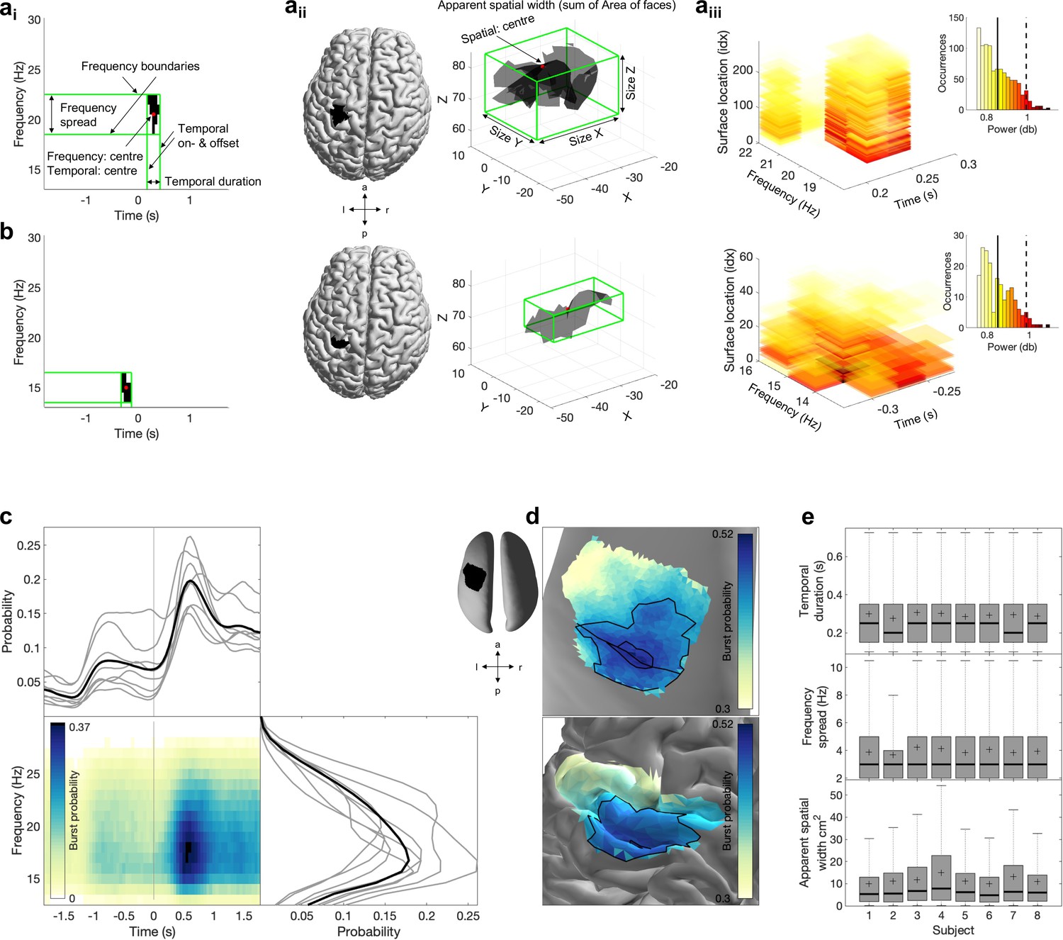
Spectral, temporal, and spatial beta burst characteristics.
(a) Burst characteristics for a single example burst. (ai) Temporal and spectral burst characteristics. (aii) Spatial burst characteristics. (aiii) Burst amplitude. Shown is the amplitude for each temporal, spectral, and spatial location of that burst, as well as the histogram across all three signal domains. Note that we use integer indexation of 3D surface location (idx) for visualisation here. All other analyses use the actual 3D surface location as provided by Cartesian x,y,z coordinates. Usually the mean (straight line) or the 95 percentile (dashed line) is reported as burst amplitude. (b) Same as (a) for a different burst. (c) Burst probability (i.e. number of bursts relative to the number of epochs) as a function of time and frequency across all bursts of all subjects (see Figure 1—figure supplement 1 for individual subjects). Burst probability as a function of time (bottom) and frequency (left) is shown for each subject separately (grey lines) and across subjects (black line). (d) Burst probability as a function of space across all bursts of all subjects on the inflated surface (top) and original surface (bottom). Highlighted are the central sulcus and the borders for 0.44 and 0.49 burst probability. To visualise burst probability as a function of space across subjects, individual subject maps were spatially normalised, projected onto a single surface, and then averaged across subjects. Figure 1—figure supplement 1 depicts the burst probability for each subject in native space. (e) Burst temporal duration (top), frequency spread (middle), and apparent spatial width (bottom) for each subject as boxplot.
Figure 1—figure supplement 1
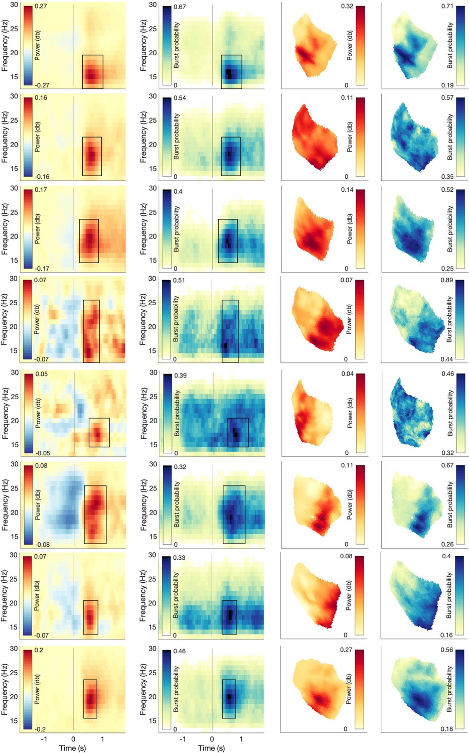
Beta power and burst probability are shown for all three signal domains for each subject.
Left: conventional beta power and burst probability are shown as a function of time and frequency. To this end, data are averaged across the region of interest (ROI). Right: conventional beta power and burst probability as a function of space averaged in time and frequency (indicated by the rectangle in the time-frequency plot).
Figure 1—figure supplement 2
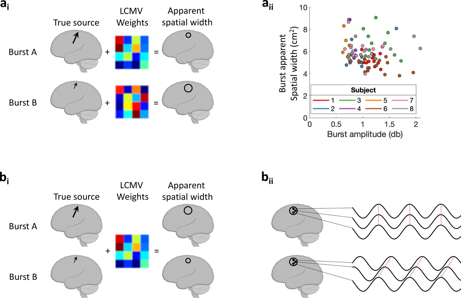
Schematic illustration of LCMV-related aspects for 3D bursts.
(ai) Schematic illustration of how differences in signal-to-noise ratio (SNR) across sessions could theoretically explain variability in bursts’ apparent spatial width. Burst A (high amplitude) and burst B (low amplitude) each with distinct linearly constrained minimum variance (LCMV) weights. If SNR across sessions explains the variability in bursts’ apparent spatial width, the apparent spatial width should be larger for small amplitude bursts. (aii) Relationship between burst amplitude and burst apparent spatial width across sessions within and across subjects. (bi) Schematic illustration of how differences in SNR within a session could theoretically explain variability in bursts' apparent spatial width. Burst A (high amplitude) and burst B (low amplitude) with shared LCMV weights. If SNR within a session explains the variability in bursts’ apparent spatial width, the apparent spatial width should be larger for high amplitude bursts. (bii) If bursts’ apparent spatial width is merely modulated by differences in SNR across bursts within a session, (1) a positive relationship between burst amplitude and burst apparent spatial width within sessions would be present, and (2) systematic phase differences across different spatial locations within each burst should be absent. Regarding the latter, if bursts’ apparent spatial width arises merely from amplitude scaling of a single source neural activity would show the same phase across different spatial locations of the burst (top). In turn, systematic phase lags across different spatial locations within the burst (bottom, Figure 5) indicate that bursts’ apparent spatial width is unlikely to arise merely from amplitude scaling of a single source.
Figure 2 with 3 supplements
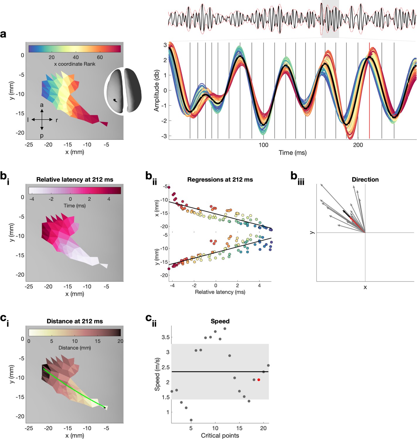
Quantification of propagation direction and propagation speed on one exemplar burst.
For a dynamic version, that is, updated for each critical point, see Figure 2—video 1. (a) Left: single burst on inflated surface. Spatial locations are colour-coded by their x coordinate rank. Note that x coordinate rank is only used here to illustrate the spatial location of the neural time series shown on the right. Right: neural activity in the beta range (13–30 Hz) from each surface location for the temporal duration of the entire epoch (top, average across spatial locations in black and amplitude-envelope in red) and in large for the temporal duration of the burst. Vertical lines indicate critical points (four critical points per oscillatory cycle, i.e. peak and trough as well as peak-trough and trough-peak midpoint) at which propagation direction and propagation speed were estimated. Red vertical line indicates the control point at 212 ms, shown in (bi,ii) and (ci,ii), and highlighted in (biii) and (ciii). (bi) Relative latencies of the critical point at 212 ms as a function of space illustrated on inflated surface. (bii) Simple linear regressions between latency at surface location and x (top) as well as y (bottom) coordinates of the surface location for the critical point at 212 ms. Colour refers to the x coordinate rank as illustrated in (a). (biii) Propagation direction obtained from regression coefficients for each critical point (grey), the critical point at 212 ms (red), and the average across all critical points (black, i.e. propagation direction of burst). (ci) Distance, that is, exact geodesic distance, from the surface location with the smallest relative latency to each surface location on the inflated surface for the critical point at 212 ms. Green line indicated the path, that is, distance, from the surface location with the smallest to the surface location with the largest relative latency. (cii) Propagation speed for each critical point (grey), the critical point at 212 ms (red). The standard deviation across critical points is indicated by the grey area, and the average across all critical points (i.e. propagation speed of burst) is indicated by the black horizontal line.
Figure 2—figure supplement 1
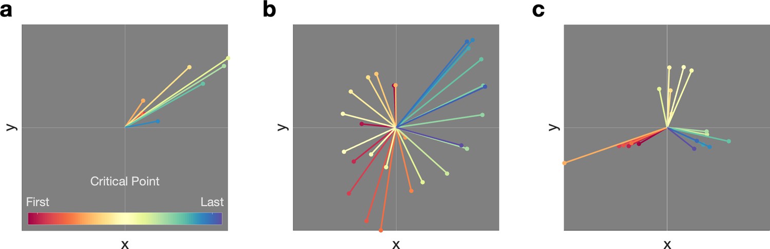
Examples of bursts with (a) one propagation direction and (b, c) complex propagation patterns.
Figure 2—figure supplement 2
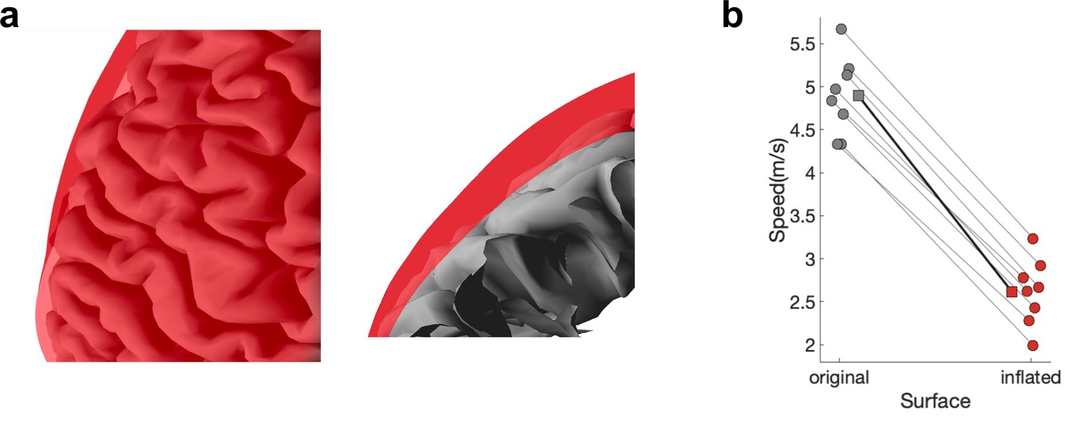
Propagation speed using the distance on the original or the inflated surface.
(a) Overlay of the original (grey) and inflated surface (red). (b) Medians are shown for each subject (circles) and the mean across the subjects’ medians (squares).
Figure 2—video 1
Same as Figure 2, but each frame corresponds to a different critical point within the burst.
Figure 3
Propagation direction can be estimated accurately from cortical meshes.
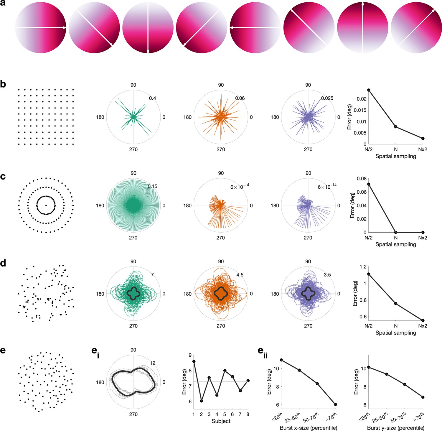
(a) Simulated gradient at 0, 45, 90, 135, 180, 225, and 270°. (b) Error between simulated gradient and estimated gradient on a square mesh. We test three different spatial sampling rates, N/2 (green), N (red), and N × 2 (blue), whereby the spatial sampling of N is roughly equivalent to the spatial sampling of the inflated surface. Error is calculated for 1–360° in steps of 1°. The median error per spatial sampling is shown in the right, that is, higher spatial sampling results in a lower error. (c) As (b), but for a circular mesh. (d) Error between simulated gradient and estimated gradient on a random mesh. 100 random meshes were generated. The error for each iteration is shown as well as the mean across iterations (black line). (e) Error between simulated gradient and estimated gradient on the inflated surface. The error was calculated for each burst. (ei) The mean across bursts is shown for each subject (grey lines) and across subjects (black line). For each subject, the mean error across all angles and bursts is shown, that is, error is comparable across subjects. (eii) Error as a function of burst size along the x-axis (left) and y-axis (right), that is, the error is lower in bigger burst.
Figure 4 with 4 supplements
Beta bursts activity propagates along one of two axes, which have distinct bursts properties.
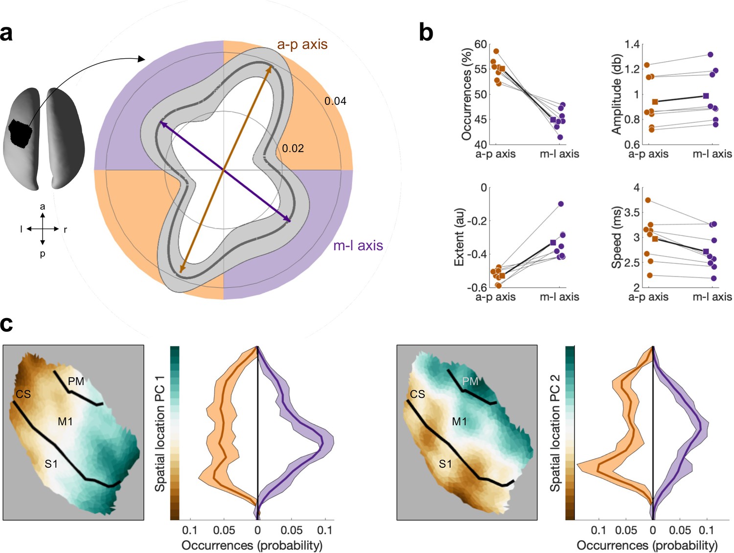
(a) Polar probability histogram showing the probability distribution of burst direction in MNI space. Probability distributions were calculated for each subject individually and then averaged (dark grey line, N=8). Variability across subjects is expressed as standard deviation from the mean (light grey area). To estimate the dominant propagation directions, a mixture of von Mises functions was fitted to the averaged probability distribution (arrows). The four functions lie on two axes. One axis has an anterior–posterior orientation which is approximately perpendicular to the orientation of the central sulcus (a-p), while the other axis runs in approximately medial–lateral orientation which is approximately parallel to the orientation of the central sulcus (m-l). (b) Burst occurrence, burst amplitude, burst extent, and burst speed differ as a function of propagation direction. Medians are shown for each subject (circles) and the mean across the subjects’ medians (squares). (c) Burst location differs as a function of burst direction. Burst location is described by two principal components (PCs) of the Cartesian coordinates of the centre of the burst. For each of the two PCs, the surface plot of the component structure and the probability distributions of the PC score are shown. Probability distributions were calculated for each subject individually and then averaged (dark line, N=8). Variability across subjects is expressed as standard deviation from the mean (light area). Bursts with a direction parallel to the CS, relative to bursts with a direction perpendicular to the CS, are located more centrally in the region of interest (ROI). CS, central sulcus; S1, primary sensory cortex; M1, primary motor cortex; PM, premotor cortex.
Figure 4—figure supplement 1
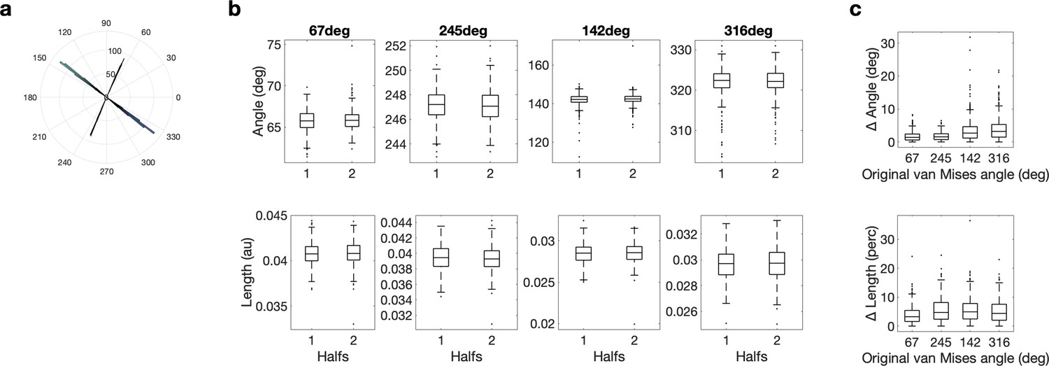
Length and angle are highly replicable for all four von Mises functions across halves of the data.
(a) Histogram of the four van Mises functions across repetitions and halves. (b) Split-half reliability for angle (top) and length (bottom) for each van Mises function. (c) Difference between the two halves for all four van Mises functions. For angle, the angular difference (top) and for length the percentage difference in length (bottom) is reported.
Figure 4—figure supplement 2
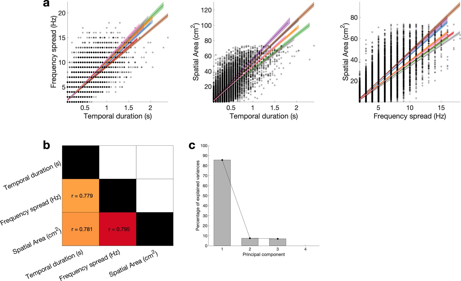
Reducing temporal duration, frequency spread, and apparent spatial width to burst extend using principal component analysis (PCA).
(a) Temporal duration, frequency spread, and apparent spatial width are highly correlated across bursts. Coloured lines represent the least-squares fit for each subject, and shaded areas indicate 95% confidence intervals. (b) Correlation matrix, whereby the Pearson correlation is averaged across subjects within each cell. (c) Variance explained by each principal component.
Figure 4—figure supplement 3
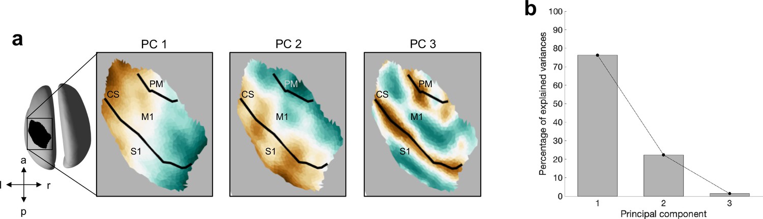
The spatial location of a burst can be summarised by the first two principal components (PCs) of the Cartesian coordinates of the centre of the burst.
(a) For each PC, the surface plot of the component structure is shown. CS, central sulcus; S1, primary sensory cortex; M1, primary motor cortex; PM, premotor cortex. (b) Variance explained by each principal component.
Figure 4—figure supplement 4
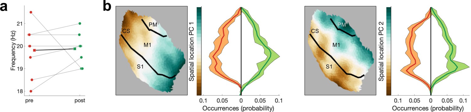
Burst frequency and burst location are comparable for pre-movement and post-movement bursts.
Frequency centre (a) and spatial location (b) and were not significantly different between pre-movement (red) and post-movement (green) bursts. CS, central sulcus; S1, primary sensory cortex; M1, primary motor cortex; PM, premotor cortex.
Figure 5

Differences in pre- and post-movement beta bursts.
(a) Burst timing relative to the button press across all subjects. Each horizontal line represents one burst. Bursts are sorted by burst onset and burst duration using multiple-level sorting, yielding the burst index. Pre-movement bursts (i.e. bursts that start and end prior to the button press) are highlighted in red, post-movement bursts (i.e. bursts that start after the button press) are highlighted in green, and bursts that start prior to the button press and end after the button press are highlighted in black. (b) Number of bursts, burst amplitude, burst extent, and burst speed differ between pre- and post-movement bursts. Medians are shown for each subject (circles) and the mean across the subjects’ medians (squares). (c) Propagation direction does not differ between pre- and post-movement bursts. Shown are polar probability histograms separately for pre- and post-movement bursts. Probability distributions were calculated for each subject individually and then averaged (dark line, N=8). Variability across subjects is expressed as standard deviation from the mean (light area). Von Mises functions were fitted separately for pre- and post-movement bursts.
Figure 6 with 2 supplements
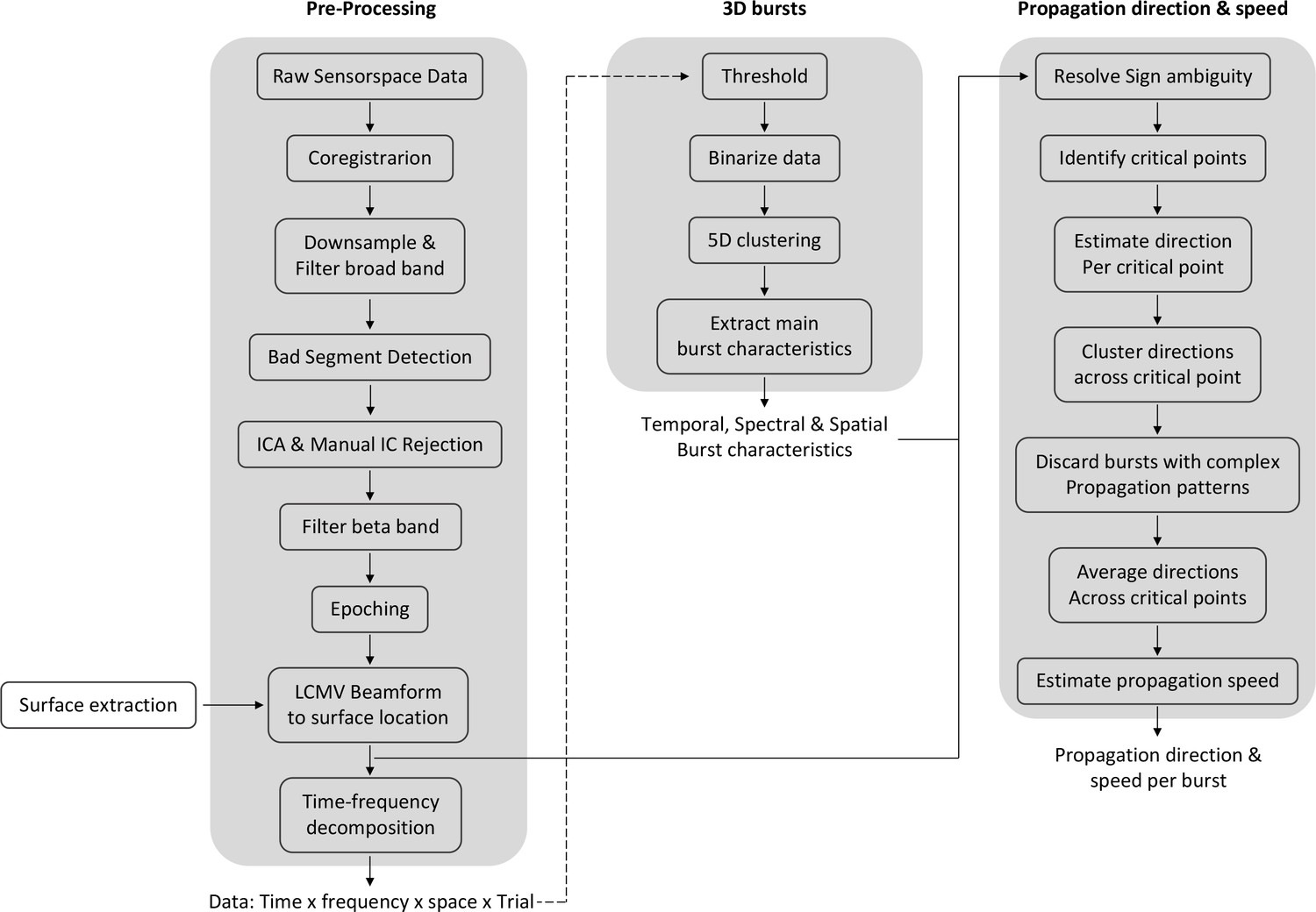
A schematic for the processing pipeline.
Figure 6—figure supplement 1
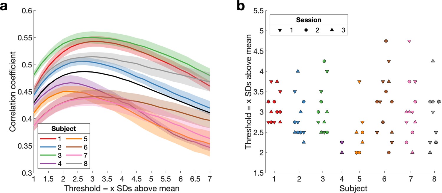
Empirical threshold to binarise beta bursts.
To account for difference in signal-to-noise across sessions, days and subjects we obtained one threshold per session. (a) Mean correlation curves across days for each subject and sessions (± SEM) and across subjects (black line). (b) Empirical threshold for each session.
Figure 6—figure supplement 2
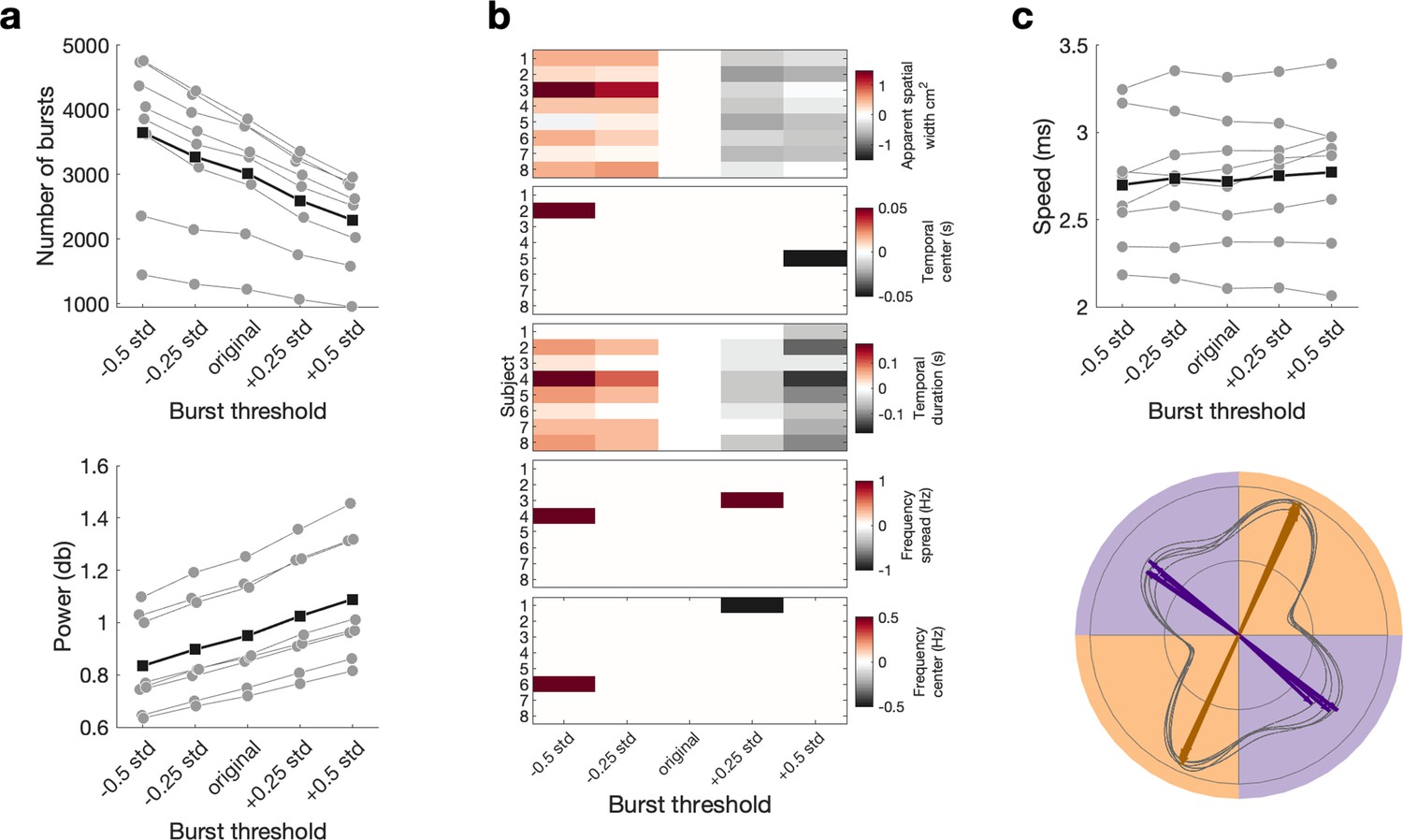
Effect of different burst thresholds on burst characteristics, propagation speed and direction.
(a) Higher thresholds lead to fewer bursts (top) and higher burst amplitudes (bottom). Medians are shown for each subject (grey) and the mean across the subjects’ medians (black). (b) Burst threshold changes the temporal duration and apparent spatial width, but not the temporal centre, frequency spread or frequency centre. For each burst characteristic and each subject, the difference from the original threshold to the other thresholds is shown. (c) Burst threshold does not affect propagation speed or propagation direction. For propagation speed (top), medians are shown for each subject (grey) and the mean across the subjects’ medians (black). The propagation direction is visualised as in Figure 4a. with the polar probability histogram showing the probability distribution of burst direction in MNI space. Probability distributions were calculated for each subject individually and then averaged. Each line represents the distribution for one of the five thresholds. The dominant propagation directions were estimated using a mixture of von Mises functions (arrows).
Author response image 1
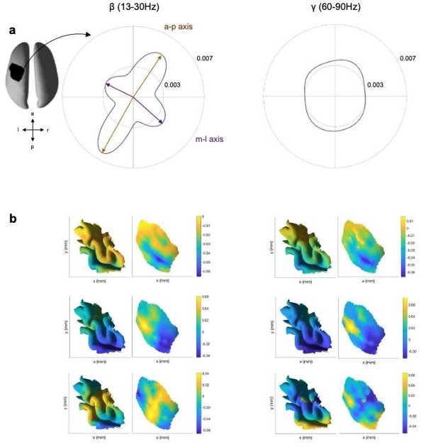
Propagation direction and LCMV weights for the β and γ frequency range.
(a) Propagation direction for the β (β, 13-30Hz) and γ (γ, 60-90) frequency range for one exemplar subject (across all sessions of that subject). (b) First three PCs of the LCMV beamformer leadfields for the β (left) and γ (right) frequency range for one session from the same subject as in a visualised on the folded and inflated.
Author response image 2
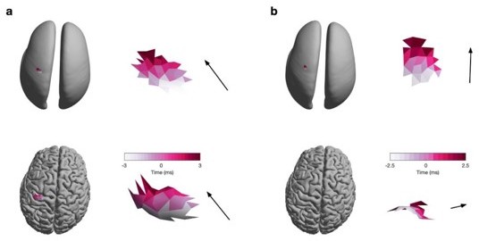
Propagation direction estimated from the original (i.e., folded) and inflated surface.
(a) Burst on the crown of the precentral gyrus visualised on the inflated (top) and original (bottom) surface. Colour denotes the relative latency of the neural activity at a critical point and the arrow indicates the estimated direction of travel (as described in the Methods section of the manuscript as well as Figure 2). (b) Same as (a) for a burst on the bank of the precentral gyrus.
Author response image 3

Cortical folding and propagation direction.
(a) Surface plot, on the inflated surface, of cortical depth, i.e. spatial location principal component (PC) 3 (see Figure 4—figure supplement 3, for PC 1 and PC 2). CS, Central Sulcus. S1, Primary Sensory Cortex. M1, Primary Motor Cortex. PM, Premotor Cortex. (b) Propagation direction does not differ as a function of cortical depth. Polar probability histograms are shown for deep (brown) and shallow (cyan) bursts. Probability distributions were calculated for each subject individually and then averaged (dark line). Variance across subjects is expressed as standard deviation from the mean (shaded area). Von Mises functions were fitted separately for deep and shallow bursts. (c) Inter-individual differences in cortical folding in the motor area. Three exemplary surfaces are shown. For the region of interest cortical depth is colour-coded (note that on the folded surface only the crown, i.e., cyan, parts are visible).
Author response image 4

Propagation direction of a subsample of bursts.
(a) Burst probability as a function of space across all bursts of all subjects on the inflated surface (top) and original surface (bottom). Unlike Figure 2d we focus here on the area of the ROI that has a burst probability higher than 0.44. Highlighted are the central sulcus and the borders for 0.44 and 0.49 burst probability. (b) Burst probability of a subset of burst forming a uniform spatial distribution across the area of the ROI that has a burst probability higher than 0.44. (c) Polar probability histogram for the subset of bursts showing the probability distribution of burst direction in MNI space. Probability distributions were calculated for each subject individually and then averaged (dark grey line). Variability across subjects is expressed as standard deviation from the mean (light grey area). To estimate the dominant propagation directions, a mixture of von Mises functions was fitted to the averaged probability distribution (arrows). The four functions lie on two axes. One axis has an anterior-posterior orientation which is approximately perpendicular to the orientation of the central sulcus (a-p), while the other axis runs in approximately medial-lateral orientation which is approximately parallel to the orientation of the central sulcus (m-l). Similar to Figure 4a.
Videos
Video 1
Illustration of 5D clustering.
Additional files
Download links
A two-part list of links to download the article, or parts of the article, in various formats.
Downloads (link to download the article as PDF)
Open citations (links to open the citations from this article in various online reference manager services)
Cite this article (links to download the citations from this article in formats compatible with various reference manager tools)
Spatiotemporal organisation of human sensorimotor beta burst activity
eLife 12:e80160.
https://doi.org/10.7554/eLife.80160


