State-dependent coupling of hippocampal oscillations
- European Brain Research Institute, Italy
- Donders Institute for Brain, Cognition and Behavior, Radboud University, Netherlands
- CNR, Institute of Molecular Biology and Pathology, Italy
Figures
Figure 1 with 2 supplements
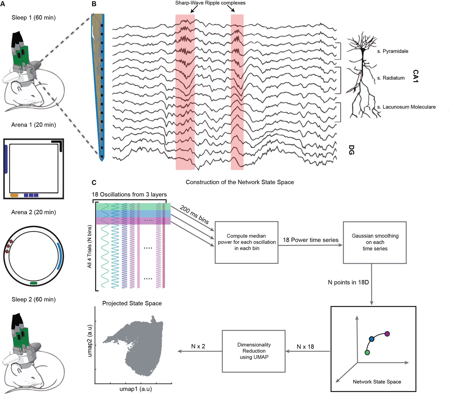
Experimental paradigm and pipeline for construction of the network state space.
(A) Representative four-trial sequence for recording during sleep and awake exploration (top to bottom). (B) Representative traces of local field potential (LFP) recorded from various layers of dorsal CA1 using silicon probe. (C) Pipeline for the construction of network state space. See also Figure 1—figure supplements 1 and 2.
Figure 1—figure supplement 1
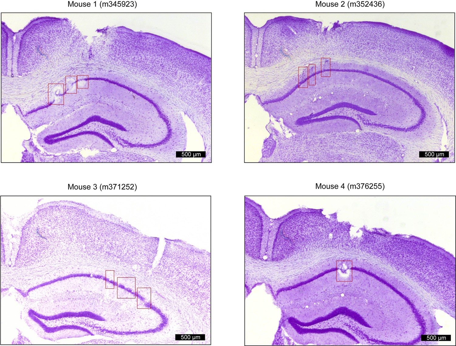
Positions of tetrodes targeting dorsal CA1 in freely moving mice.
Four representative Nissl-stained coronal section showing recording locations from each animal (mouse 1,2,3,4). Red squares indicate the estimated location (CA1 pyramidal layer) of tetrode tips after electrolytic lesions.
Figure 1—figure supplement 2

Accelerometer signal in arbitrary units overlaid on network state space used for the identification of sleep states during rest periods.
Figure 2 with 4 supplements
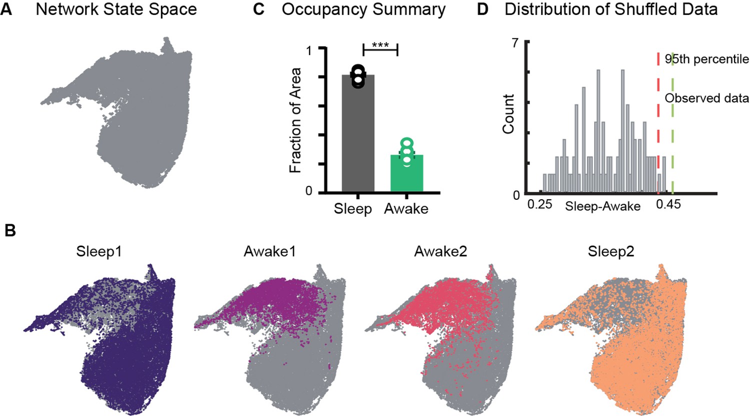
Restricted occupancy of the network state space during wakefulness.
(A) Network state space for all four trials combined. (B) Trial-specific states (colored) and unvisited states (gray) on the network state space. (C) Fraction of state space occupied during sleep and awake trials, suggesting significant restrictions during awake trials (n = 8 sleep and awake trials from four mice. p=0.0002, Mann–Whitney test). (D) Distribution of difference in fraction of state space occupied during sleep and awake trials (Sleep-Awake) of surrogate data and observed data. See also Figure 2—figure supplements 1–4.
Figure 2—figure supplement 1
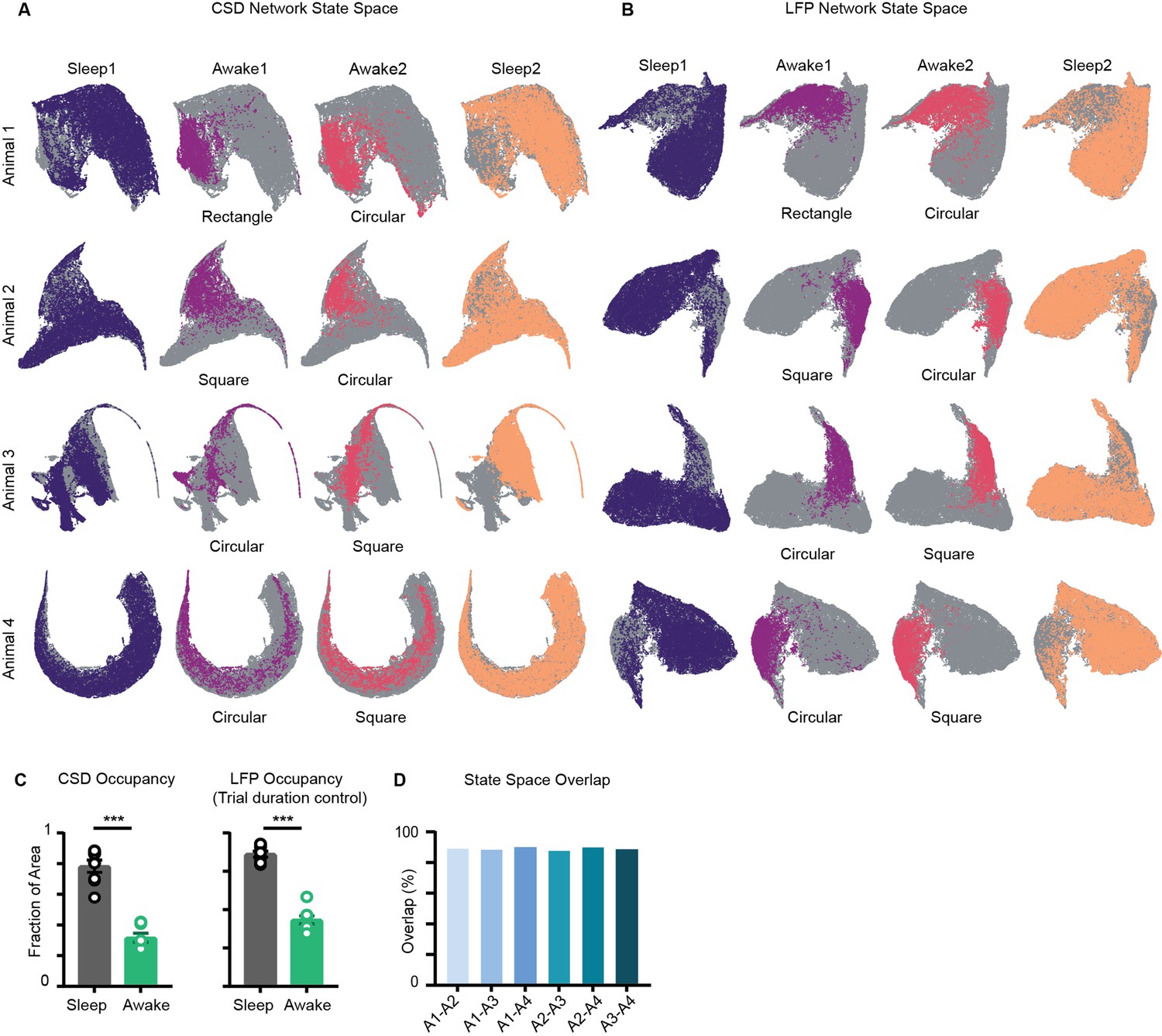
Trial-specific states overlaid on current source density (CSD) and local field potential (LFP) network state space.
(A) Network state space constructed using power in CSD signals, instead of LFP for four animals. Unvisited states are colored in gray. Trail specific states are colored. (B) Network state space constructed using power in LFP signals for the four mice. (C) Left: fraction of state space occupied on CSD state space Sleep v/s Wake Right: fraction of state space occupied on LFP state space obtained by combining equal number of states from sleep and awake trial, controlling for difference in trial duration (p=0.0002, Mann–Whitney test). (D) State space occupancy overlap among four animals (mice A1, A2, A3, A4) suggesting similarity of states across animals. Overlap computed by projecting the individual state space on the same axis.
Figure 2—figure supplement 2

Network state space (local field potential [LFP]) computed with standardized features (z-scored).
(A) State space from four mice and trial-specific states overlaid on it (colored). (B) Fraction of area occupied on normalized state space Sleep v/s Awake , p=0.0002, Mann–Whitney test.
Figure 2—figure supplement 3
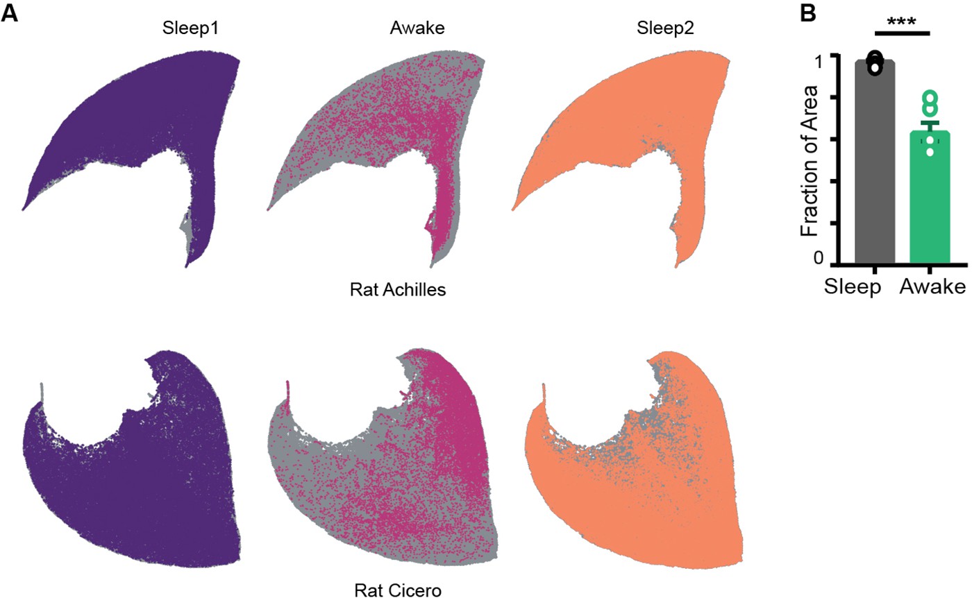
Restricted occupancy on the network state space in rats.
(A) Representative network state space from two rats (gray) and states occupied during sleep and awake trials. Datasets obtained from crcns.org courtesy of Dr. Gyorgy Buzsaki’s lab at NYU. (B) Fraction of area computed from rat datasets. Sleep v/s Awake , p=0.0001, Mann–Whitney test (n = 12 sleep and 6 awake trials from three rats).
Figure 2—figure supplement 4
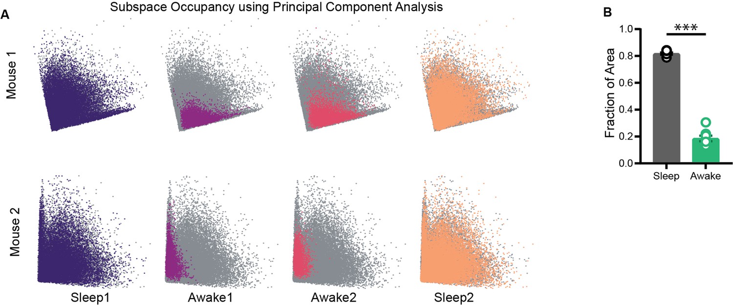
Subspace occupancy visualized using principal component analysis (PCA).
(A) Representative network state space of two mice projected on 2D plane using PCA (~80% variance explained). Note that the visualization of restrictions on the state space is independent of the dimensionality reduction method employed. (B) Fraction of area occupied as computed on projections obtained using PCA. Sleep (0.81 ± 0.008) versus Awake (0.18 ± 0.02), p=0.0002, Mann–Whitney test (n = 8 sleep and 8 awake trials from four mice).
Figure 3
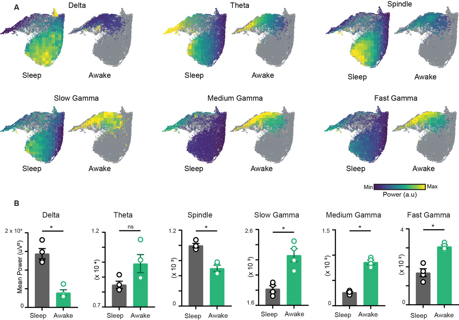
Characterization of restrictions on the network state space during wakefulness.
(A) Distribution of power on state space for six oscillations of layer stratum pyramidale: delta (1–5 Hz), theta (6–10 Hz), beta (10–20 Hz), slow gamma (20–45 Hz), medium gamma (60–90 Hz), and fast gamma (100–200 Hz). Each oscillation is individually color-scaled to its respective minimum and maximum power. Unvisited states are in gray. The overlay maps demonstrate how the power of each oscillation varies on the state space and across sleep and awake trials. (B) Mean power comparison between awake and sleep trials using classical approach (n = 4 mice). All p<0.05, except for theta (p=0.11), Mann–Whitney test.
Figure 4 with 1 supplement
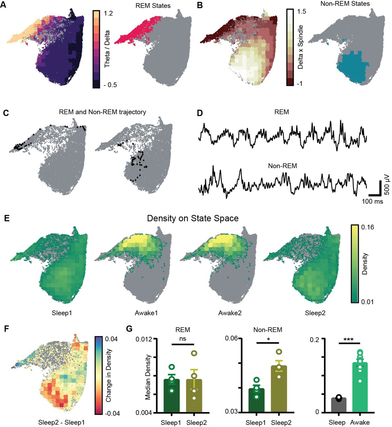
Localization of rapid eye movement (REM) and non-REM sleep states and density on the network state space.
(A) Left: standardized theta/delta ratio from pyramidal layer overlaid on state space. Right: identified REM states (magenta colored). (B) Left: standardized delta × beta product from pyramidal layer overlaid on state space. Right: identified non-REM states (cyan colored). (C) Representative REM and non-REM states on the network state space. (D) Corresponding REM and non-REM local field potential (LFP) from pyramidal layer. (E) Density overlaid on state space across all four trials (unvisited states are colored gray). (F) Representative change in density map across two sleep trials (Sleep2 – Sleep1). (G) Left: comparison of median REM density between two sleep trials (n = 4 mice); (Sleep1: v/s Sleep2: 0.0075 ± 0.001, p=0.88 Mann–Whitney test); Center: comparison of median non-REM density between two sleep trials (n = 4 mice); (Sleep1: 0.039 ± 0.001 v/s Sleep2: 0.048 ± 0.002, p<0.05, Mann–Whitney test); right: median density comparison between and sleep and awake trials (n = 8 sleep and awake trials, four mice) (0.03 ± 0.0005 v/s 0.13 ± 0.009, p=0.0002 Mann–Whitney test). See also Figure 4—figure supplement 1.
Figure 4—figure supplement 1
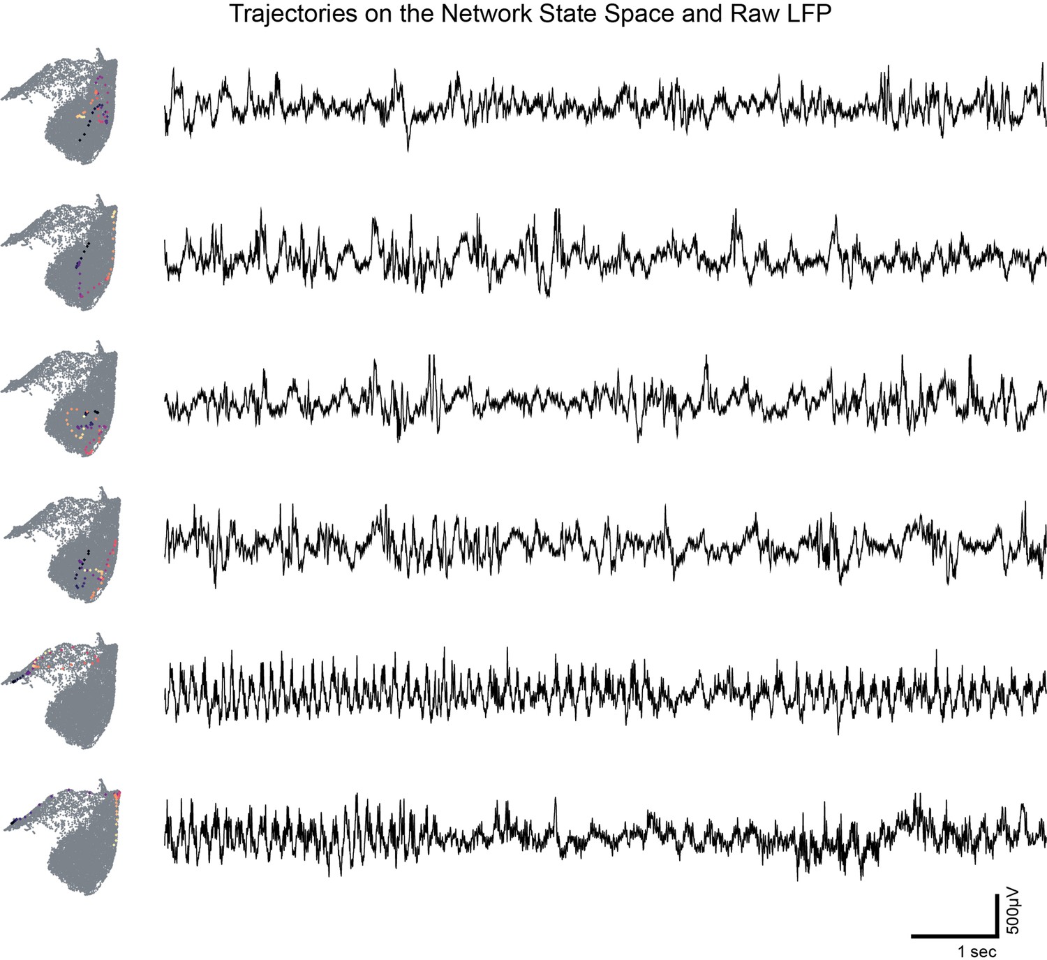
Trajectories on the network state space and raw local field potential (LFP) from CA1 pyramidal layer.
Representative examples of network trajectory the state space (10 s, starting from blue to yellow) and corresponding local field potentials from CA1. Note the presence of different oscillatory bands in raw LFP.
Figure 5
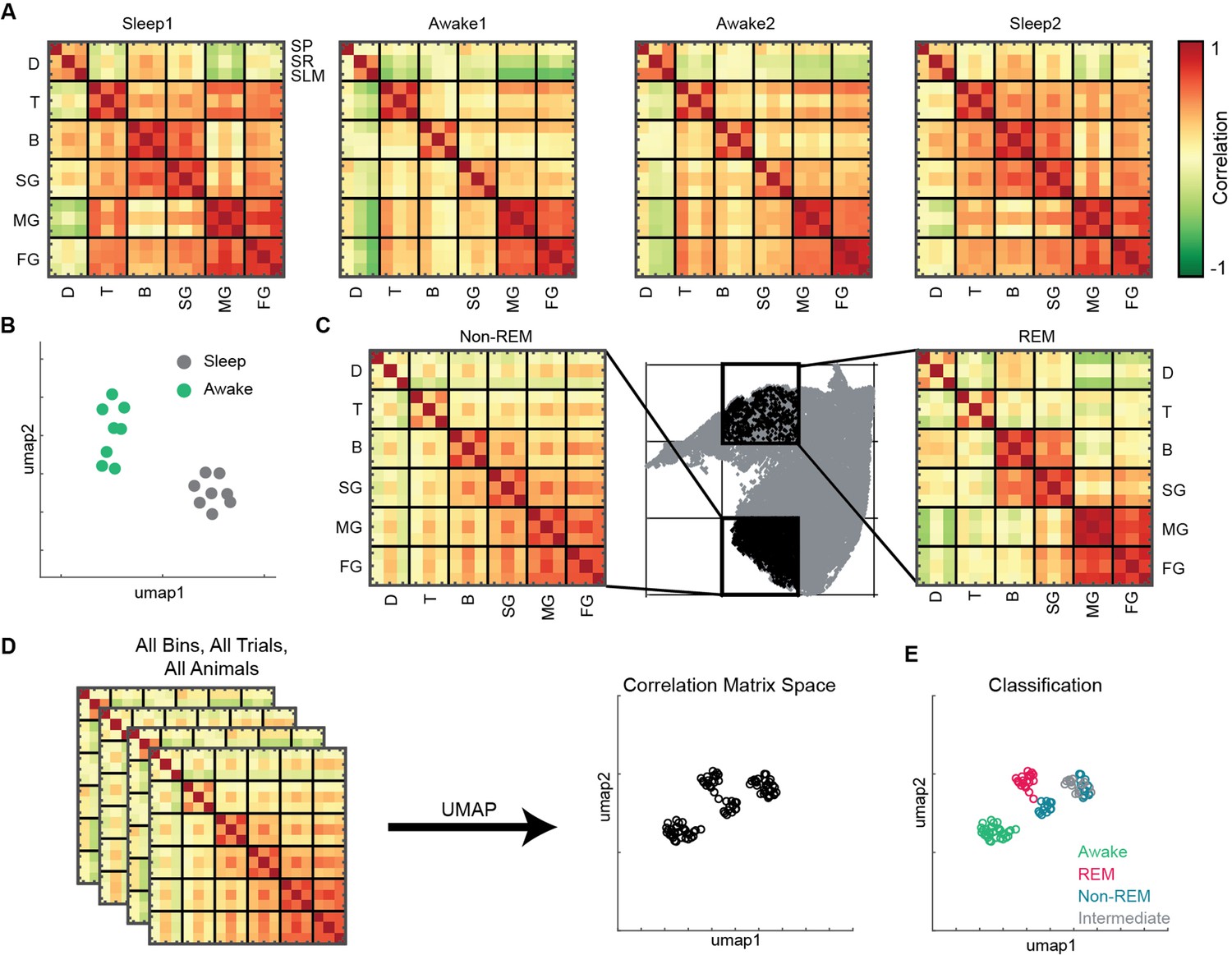
State and layer-dependent coupling of hippocampal oscillations.
(A) Representative pairwise correlation among 18 oscillations (D, delta; T, theta; B, beta; SG, slow gamma; MG, medium gamma; FG, fast gamma) from three layers (stratum pyramidale [SP], stratum radiatum [SR], stratum lacunosum moleculare [SLM]). Rows are arranged by combining all three layers for each oscillation. (B) Correlation matrix space generated by using matrices in (A) from all the mice (total 16 points, 8 sleep and 8 awake trials from four mice). Each point represents the correlation matrix of oscillations. The separation of sleep and awake points in the correlation matrix space suggests distinct nature of coupling among oscillations during sleep and wakefulness. (C) Binned state space (gray) for a sleep trial. Representative rapid eye movement (REM) and non-REM bins highlighted (black) and their corresponding correlation matrix of oscillations. (D) Correlation matrix space constructed using matrices from all bins collected from all trials and all animals. Each point on correlation matrix space projection represents a correlation matrix. (E) Bin status (awake, REM, non-REM, intermediate sleep) overlaid on correlation matrix space, exhibiting state dependent coupling of hippocampal oscillations (p<0.0001 using multivariate ANOVA).
Figure 6 with 2 supplements
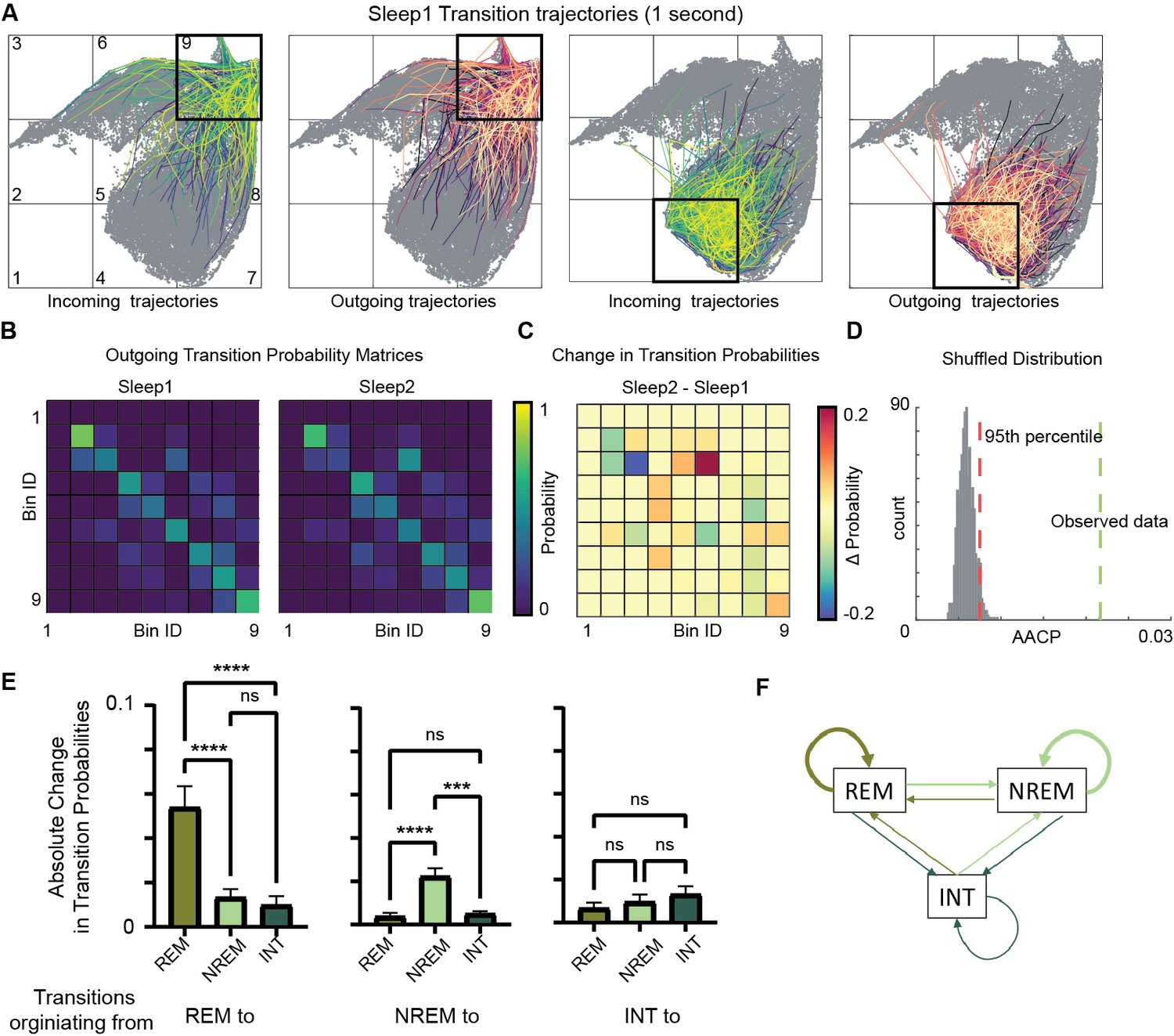
Alterations in sleep state transitions after exploration.
(A) Incoming and outgoing trajectories for two representative bins on state space during a sleep trial. Each trajectory spans 1 s in time before (incoming) and after (outgoing) the occurrence of a given state in each bin. (B) State transition matrices for two sleep trials: pre-exploration sleep (Sleep1) and post-exploration sleep (Sleep2). (C) Change in transition probabilities across two sleep trials obtained by subtracting two transition matrices (Sleep2 – Sleep1). (D) Comparison of observed sleep data’s average absolute change in probability with shuffled sleep data. Average absolute change in probability (AACP) across sleep trials for observed data = 0.021, 95th percentile of shuffled data = 0.007. (E) AACP across sleep trials for transitions originating from rapid eye movement (REM), non-REM, and intermediate (INT) state to REM, non-REM, and intermediate sleep state (REM: p<0.0001; non-REM: p<0.0001; INT: p=0.38, one-way ANOVA). (F) Schematic diagram of absolute change in transition probabilities across sleep trials. Arrow’s thickness corresponds to absolute change in transition probabilities. See also Figure 6—figure supplements 1 and 2.
Figure 6—figure supplement 1
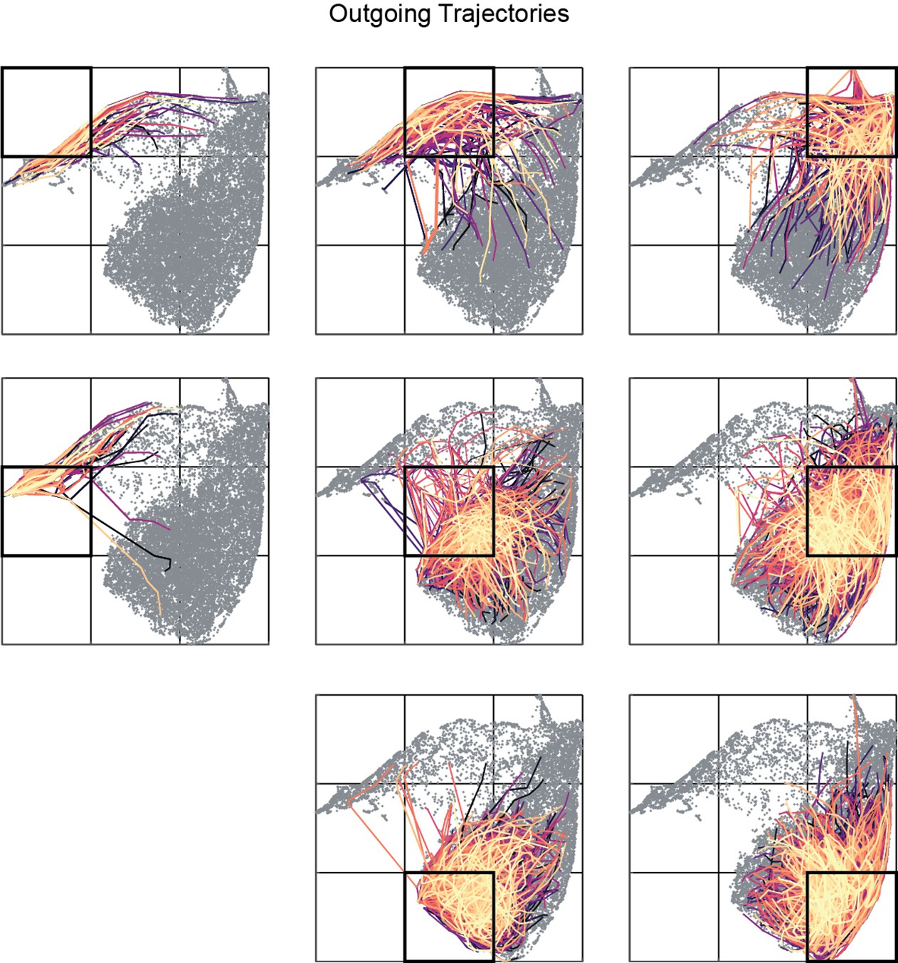
Outgoing trajectories (1 s in future) for all bin of a representative sleep trial.
Distinct colors correspond to trajectories originating from distinct states in a given bin (highlighted in black).
Figure 6—figure supplement 2

Comparison of average absolute change in probability (AACP) of transition matrices with shuffle data.
(A, B) Comparison of observed data’s AACP computed for rapid eye movement (REM)-to-REM and non-REM to non-REM transitions across sleep trials with shuffled data.
Figure 7 with 1 supplement
Network stabilization during transition to rapid eye movement (REM).
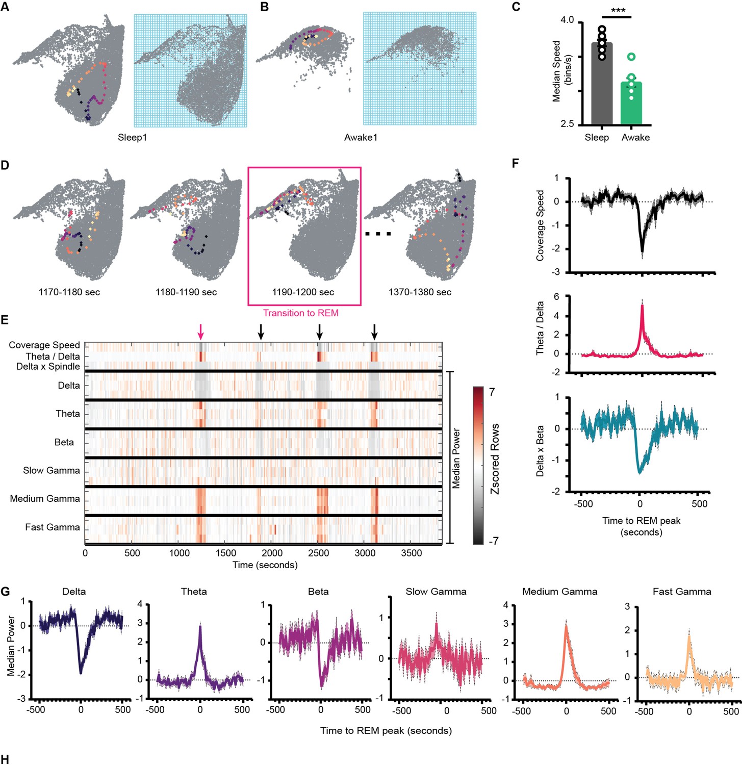
(A) Left: representative trajectory in 10 s time frame on state space during sleep trial (trajectory starts from blue to yellow). Right: binned state space used to compute the speed. (B) Same as (A), but for awake trial. (C) Median speed for sleep and awake trials (n = 8 awake and sleep trials from four animals) (Sleep: 3.7 ± 0.04 v/s Awake: 3.12 ± 0.06 bins/s), p=0.0003, Mann–Whitney test. (D) Representative trajectories in 10 s time frame before (panels 1 and 2) network transitions to REM state (panel 3, red box), and when network exits REM (panel 4). (E) Median power v/s time for entire sleep trial with 18 oscillations, speed of coverage, theta/delta ratio, and delta × beta product. Arrows indicate network transition to REM. Red arrow corresponds to example shown in (D). Each row is independently z-scored. Three rows for given oscillation corresponds to three layers (stratum pyramidale, radiatum, and lacounosum-moleculare, respectively). Note the changes in median power of oscillations as network transition to REM. (F) Summary plot for 19 REM bouts collected across eight sleep trials from four mice. Top: speed of coverage (units: bins/s) center: theta/delta ratio bottom: delta × beta power product showing dip in coverage speed as network transitions to REM. All plots are standardized using z-score. (G) Average power for six oscillations from pyramidal layer for 19 REM bouts as network transitions to REM. All are statistically significant at T = 0 s when compared with T = –500 s except slow gamma, p<0.05, Mann–Whitney test. See also Figure 7—figure supplement 1.
Figure 7—figure supplement 1

Speed of coverage on normalized state space.
(A) Top: speed of coverage on normalized state space during transition to rapid eye movement (REM). Center and bottom: theta/delta power ratio and delta × beta power product (same as Figure 7F). (B) Median speed of coverage computed on normalized state space for sleep and awake trials (Sleep v/s Awake ) bins/s. p=0.0002, Mann–Whitney test.
Figure 8 with 5 supplements
Distinct sleep state signatures for cells with different firing rates and sparsity.
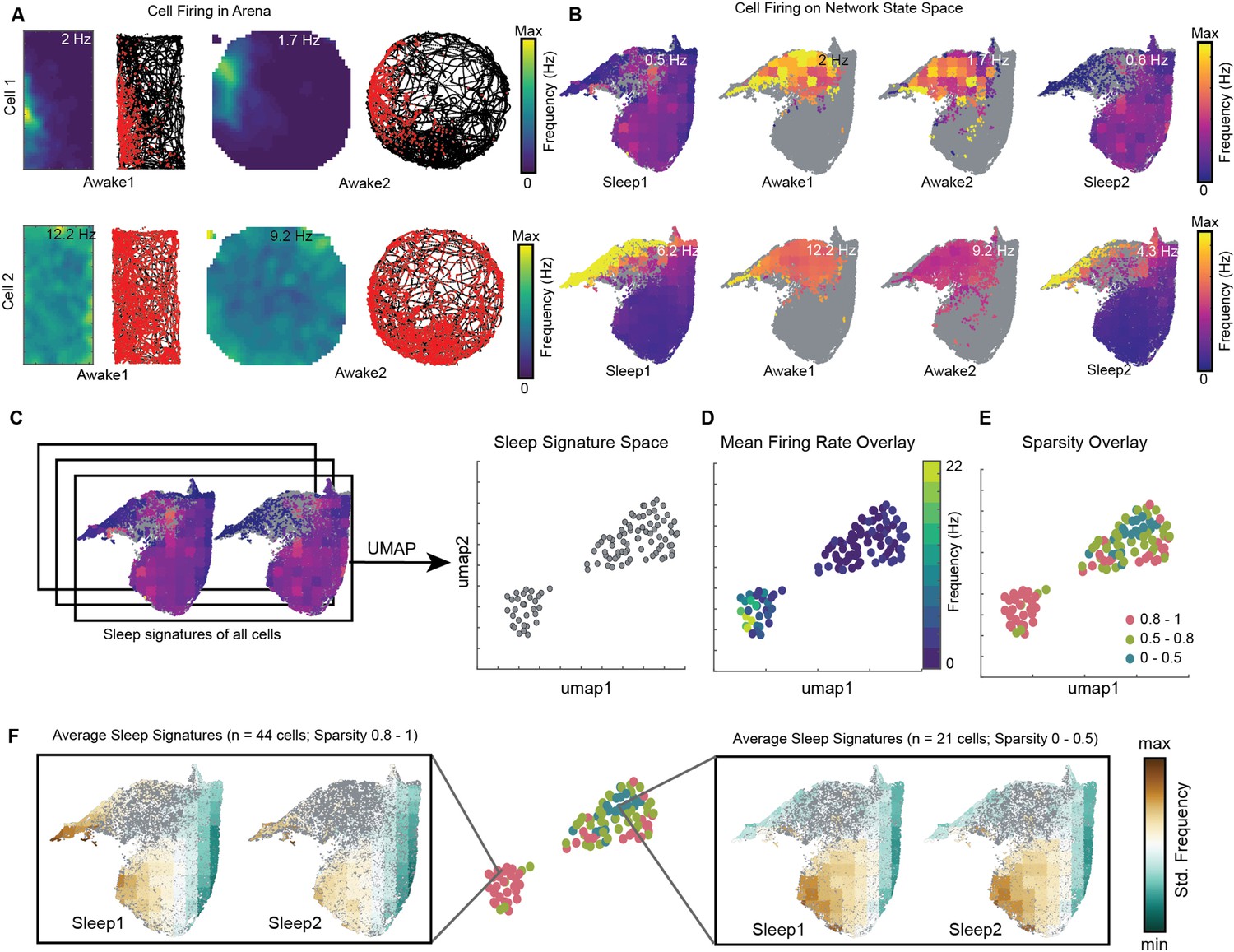
(A) Two representative cells and their firing during awake exploration trials (rectangle and circular arena). Panels 1 and 3 in both rows: firing rate map for two trials. Panels 2 and 4: animal’s trajectory during exploration (black) and overlaid with spikes (red). (B) Firing of cells across four trials overlaid on network state space. Unvisited states are colored gray. Note that the distinct cell firing patterns in arenas correspond to distinct cell firing patterns on network state space. (C) Sleep signatures on state space are used to create signature space with 106 cells from a given animal. Each point represents firing signature of cell on state space across two sleep trials. (D, E) Mean firing rate and mean sparsity as observed during two awake trials, overlaid on sleep signature space. Note that most high-firing cells on the opposite end of the spectrum from low-firing cells suggesting distinct sleep signature for cells having distinct firing rates and sparsity during awake exploration. (F) Average sleep signatures for two sets of cells having low (0–0.5) and high sparsity (0.8–1) during awake exploration. See also Figure 8—figure supplements 1–5.
Figure 8—figure supplement 1
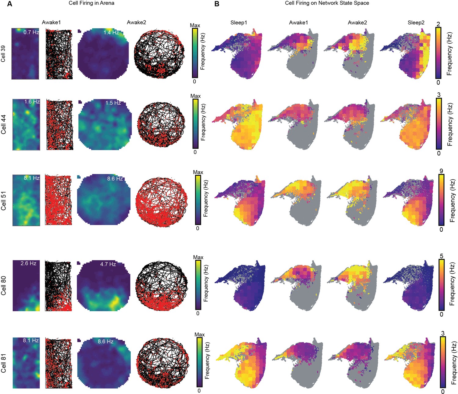
Cell firing overlaid on arenas during exploration and on the network state space.
(A) Representative cells with rate maps, spikes (red), and trajectory(black) on two arenas during awake exploration. (B) Corresponding cell firing rate overlaid on the network state space during four trials.
Figure 8—figure supplement 2

Distinct sleep signature corresponds to cells with distinct firing patterns in arena.
(A, B) Mean firing rate and mean sparsity as observed during two awake trials, overlaid on projected sleep signature space. A total of 115, 93, and 76 isolated units from CA1 pyramidal layer of mouse 2, 3, and 4, respectively.
Figure 8—figure supplement 3
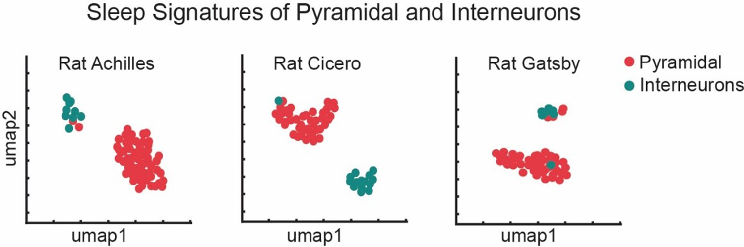
Distinct sleep signature corresponds to distinct cell types in hippocampus.
Analysis of hc-11 dataset reveals that pyramidal and interneurons in hippocampal CA1 are modulated by distinct set of oscillations during sleep. We analyzed three rats: Rat Achilles (9 interneurons, 63 pyramidal neurons), Rat Cicero (15 interneurons, 42 pyramidal neurons), and Rat gGatsby (7 interneurons, 48 pyramidal neurons). Sleep signatures and Uniform Manifold Approximation and Projection (UMAP) are obtained by the methods used for generating Figure 8C.
Figure 8—figure supplement 4
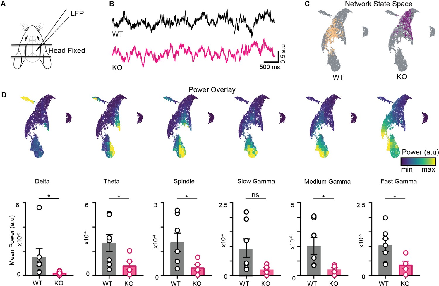
Altered organization of hippocampal oscillations in NLG3 KO mice.
(A) Experimental paradigm: local field potential (LFP) recordings from hippocampal CA1 of head-fixed mice at rest on a platform. (B) Sample LFP traces obtained from WT (black) and KO (pink) mice. (C) Combined network state space obtained by merging data from all trials and all animals (gray). Sample trial of WT and KO mice overlaid on combined network state space. (D) Top: power overlay on network state space for 6 oscillations of CA1. Bottom: mean power comparison of individual bands. (WT vs. KO, all power in arbitrary units). Delta ; theta (); beta ; slow gamma ; medium gamma ; fast gamma ; Mann–Whitney test (all p<0.05 except for slow gamma).
Figure 8—figure supplement 5
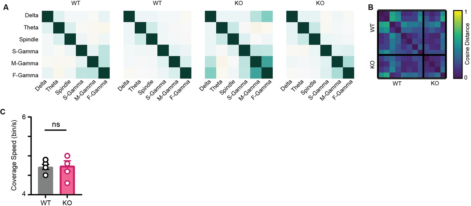
Characterization of state space in WT and NLG3 KO mice.
(A) Representative correlation matrix of oscillations from two trials of WT and KO mice. (B) Pairwise cosine distance between correlation matrices from seven trials of WT and five trials of KO mice. Note the similarity among matrices across genotypes. (C) Mean coverage speed for WT and KO mice (n = 7 WT trials and 5 NLG3 KO trials) , p=0.9, Mann–Whitney test.
Additional files
Download links
A two-part list of links to download the article, or parts of the article, in various formats.
Downloads (link to download the article as PDF)
Open citations (links to open the citations from this article in various online reference manager services)
Cite this article (links to download the citations from this article in formats compatible with various reference manager tools)
State-dependent coupling of hippocampal oscillations
eLife 12:e80263.
https://doi.org/10.7554/eLife.80263


