Rapid learning of predictive maps with STDP and theta phase precession
- Sainsbury Wellcome Centre for Neural Circuits and Behaviour, University College London, United Kingdom
- Research Department of Cell and Developmental Biology, University College London, United Kingdom
- DeepMind, United Kingdom
Figures
Figure 1
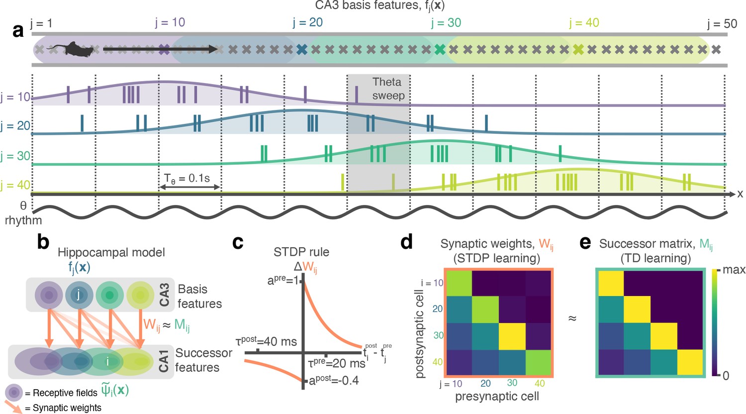
STDP between phase precessing place cells produces successor representation-like weight matrices.
(a) Schematic of an animal running left-to-right along a track. 50 cells phase precess, generating theta sweeps (e.g. grey box) that compress spatial behaviour into theta timescales (10 Hz). (b) We simulate a population of CA3 ‘basis feature’ place cells which linearly drive a population of CA1 ‘STDP successor feature’ place cells through the synaptic weight matrix . (c) STDP learning rule; pre-before-post spike pairs () result in synaptic potentiation whereas post-before-pre pairs () result in depression. Depression is weaker than potentiation but with a longer time window, as observed experimentally. (d) Simplified schematic of the resulting synaptic weight matrix, . Each postsynaptic cell (row) fires just after, and therefore binds strongly to, presynaptic cells (columns) located to the left of it on the track. (e) Simplified schematic of the successor matrix (Equation 3) showing the synaptic weights after training with a temporal difference learning rule, where each CA1 cell converges to represent the successor feature of its upstream basis feature. Backwards skewing (successor features ‘predict’ upcoming activity of their basis feature) is reflected in the asymmetry of the matrix, where more activity is in the lower triangle, similar to panel d.
Figure 2 with 4 supplements
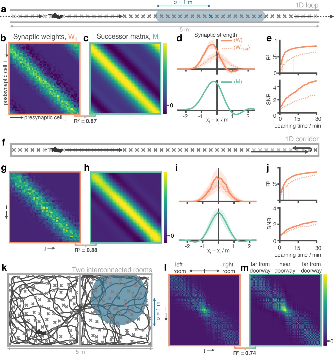
Successor matrices are rapidly approximated by STDP applied to spike trains of phase precessing place cells.
(a) Agents traversed a 5 m circular track in one direction (left-to-right) with 50 evenly distributed CA3 spatial basis features (example thresholded Gaussian place field shown in blue, radius m). (b&c) After 30 min, the synaptic weight matrix learnt between CA3 basis features and CA1 successor features strongly resembles the equivalent successor matrix computed by temporal difference learning. Rows correspond to CA1, columns to CA3. (d) To compare the distribution of weights, matrix rows were aligned on the diagonal and averaged over rows (mean ± standard deviation shown). (e) Against training time, we plot (top) the R2 between the synaptic weight matrix and successor matrix and (bottom) the signal-to-noise ratio of the synaptic matrix. Vertical lines show time where R2 reaches 0.5. (f-j) Same as panels a-e except the agent turns around at each end of the track. The average policy is now unbiased with respect to left and right, as can be seen in the diagonal symmetry of the matrices. (k-m) As in panels a-c except the agent explores a two dimensional maze where two rooms are joined by a doorway. The agent follows a random trajectory with momentum and is biased to traverse doorways and follow walls.
Figure 2—figure supplement 1
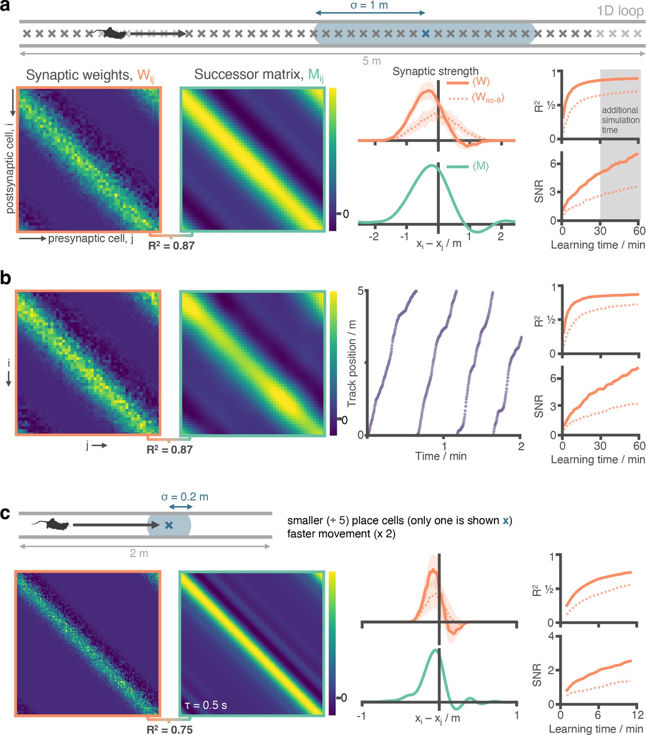
STDP and phase precession combine to make a good approximation of the SR independent of place cell size and running speed statistics.
(a) Figure 2 panels a-e have been repeated (additional 30 min simulation carried out) for ease of comparison. (b) We repeat the experiment with non-uniform running speed. Here, running seed is sampled according to a continuous stochastic process (Ornstein Uhlenbeck) with mean of 16 cm s–1 and standard deviation 16 cm s–1 thresholded to prevent negative speeds. As can be seen in the trajectory figure speed varies smoothly but significantly, including regions where the agent is almost stationary. Despite this there is no observable difference to the synaptic weights after learning. (c) We reduce the place cell diameter from 2 m to 0.4 m (5 x decrease) and increase the motion speed from 16 cm s–1 to 32 cm s–1 (2 x increase). We increase the cell density along the track from 10 cells m–1 to 50 cells m–1 to preserve cell overlap density. To reduce the computational load of training we shrink the track length from 5 m to 2 m (any additional track is symmetric and redundant when place cells are this small anyway). Note the adjusted training time: 12 min on a 2 m track at 32 cm s–1 corresponds to the same number of laps as 60 min on a 5 m track at 16 cm s–1 as shown for comparison in panel (a). Under these conditions, the STDP +phase precession learning rule well approximates the successor features with a shorter time horizon of .
Figure 2—figure supplement 2
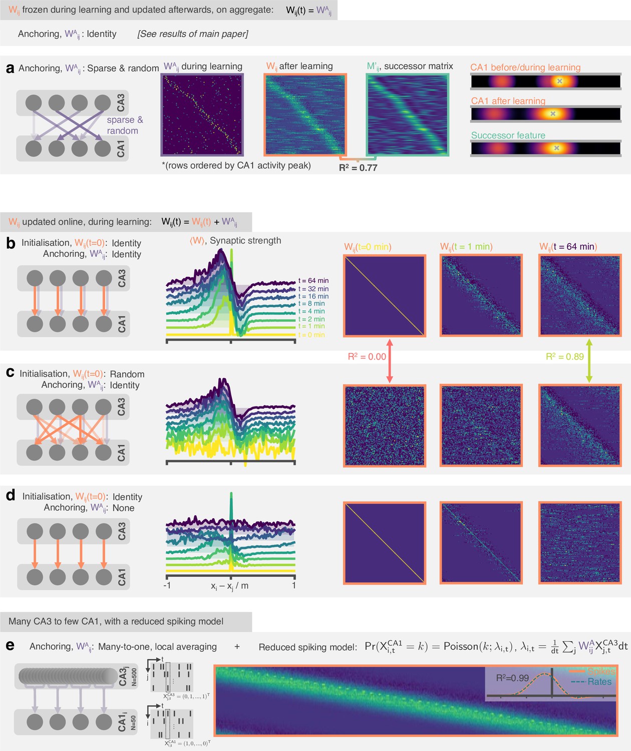
The STDP and phase precession model learns predictive maps irrespective of the weight initialisation and the weight updating schedule.
In the original model weights are set to the identity before learning and kept (‘anchored’) there, only updated on aggregate after learning. In these panels, we explore variations to this set-up. (a) (Left) Weights are anchored to a sparse random matrix, not the identity. (Middle) Three weight matrices show the random weights before/during learning, the weights once they have been updated on aggregate after learning and the successor matrix corresponding to the successor features of the mixed features. Matrix rows are ordered by peak CA1 activity location in order that some structure is visible. (Right) An example CA1 feature (top) before learning and (middle) after learning alongside (bottom) the corresponding successor feature. (b) (Left) The weight matrix is no longer fixed during learning, instead it is initialised to the identity and updated online during learning. A fixed component (0.5 x ) is added to ‘anchor’ the downstream representations. (Middle and right) After learning the STDP weights show an asymmetric shift and skew against the direction of motion and a negative band ahead of the diagonal just as was observed for successor matrices and the fixed weight model. This backwards expansion does not carry on extending indefinitely (a risk when the weights are updated online) but stabilises. (c) Like panel b but weights are randomly initialised. After learning the weights have ‘forgotten’ their initial structure and are essentially identical to in the case of identity initialisation. (d) Like panel b except no anchoring weights are added. Now there is no fixed component anchoring CA1 representations, structure in the synaptic weights rapidly disintegrates. (e) 500 CA3 neurons drive 50 CA neurons where each CA1 neuron is anchored to a Gaussian-weighted sum of 10 closest CA3 cells. CA3 spikes now directly drive CA1 spikes according to a reduced spiking model. The inset shows the row-averages and a comparison to the result for an equivalent simulation with the rate-model used in the rest of the paper.
Figure 2—figure supplement 3
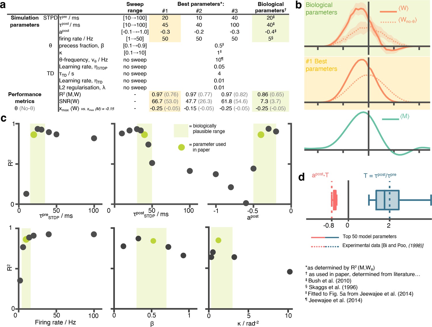
A hyperparameter sweep over STDP and phase precession parameters shows that biological parameters are suffice, and are near-optimal for approximating the successor features.
(a) A table showing all parameters used in this paper and the ranges over which the hyperparameter sweep was performed. For each parameter setting, we estimate performance metrics to judge whether the STDP parameters do well at learning the successor features. (b) Visually inspecting the row aligned STDP weight matrices, we see the optimal parameters do not significantly out perform the biologically chosen ones. Although the optimal parameter setting results in a slightly higher , they fail to capture the right-of-centre negative weights present in the TD successor matrix, unlike the biological ones. (c) Slices through the parameter sweep hypercube. For each plot, parameter values of the other five variables are fixed to the green values (i.e. are the ones used in this paper). (d) The top 50 performing parameter combination are stored and box plots for the conjugate parameter , the ratio of time windows for potentiation and depression, and , effectively the ratio of the areas under the curve left and right of the y-axis on the STDP plot Figure 1b. In both cases, the ‘best parameters’ include the true parameter values, measured experimentally by Bi and Poo, 1998.
Figure 2—figure supplement 4
Biological phase precession parameters are optimal for learning the SR.
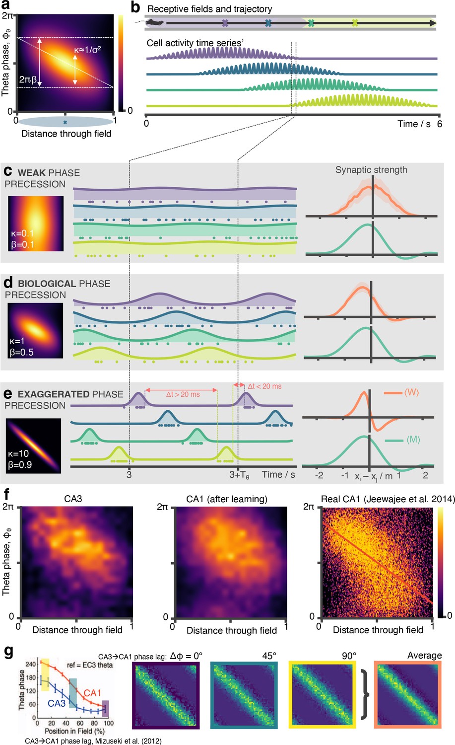
(a) We model phase precession as a von Mises centred at a preferred theta phase which precesses in time. This factor modulates the spatial firing field. It is parameterised by (von Mises width parameter, aka noise) and (fraction of full 2π phase being swept, diagonal line). We showed in a previous figure that biological phase precession parameters are optimal. Any more or less phase precession degrades performance. It is easy to understand why: (b) Consider four place cells on a track (purple, blue, green, yellow) where the first and last just overlap. (c) In the weak phase precession regime, there is no ordering to the spikes and STDP can’t learn the asymmetry in the successor matrix (right) (d) In the medium phase precession regime, spikes are broadly ordered in time (purple then blue then green…) so the symmetry is broken and STDP learns a close approximation the successor matrix (e) In the ‘exaggerated’ phase precession regime, there exist two problems for learning SRs: ‘causal’ bindings (e.g. from presynaptic purple to postsynaptic yellow, which sits in front of purple) are inhibited for anything except the most closely situated cell pairs due to the sharp tuning curves. Secondly, though this is a less important effect, when is too large it is possible for incorrect “acasual” bindings to be formed due to one cell (e.g. yellow) firing late in theta cycle N just before another cell located far behind it on the track fires (e.g. purple) in theta cycle N+1. (f) CA1 cells will phase precess when driven by multiple CA3 place cells. Here, we show phase precession (spike probability for different theta phases against distance travelled through field) for CA3 basis features and CA1 STDP successor features after learning. Although noisier, there is still a clear tendency for CA1 cells to phase precess. Real CA1 cell phase precession can be ‘noisy’; we show for comparison a phase precession plot for CA1 place field taken from Jeewajee et al., 2014, the same data for which we fitted our parameters. The schematic simulation figures showing spiking phase precession data in panels b, c, d, and e were made using an open source hippocampal data generation toolkit (George et al., 2022). Panel f, right has been adapted from Figure 5a from Jeewajee et al., 2014. (g) (Left) A decreasing phase shift is measured between CA3 and CA1, starting from 90º late in the cycle – the phase cells initially spike at as animals enter a field – and ending at 0º early in the cycle, panel adapted from Mizuseki et al., 2012. (Middle) Three phase shifts (0º, 45º and 90º) are simulated and the average of the resulting synaptic weight matrices is taken (right).
Figure 3
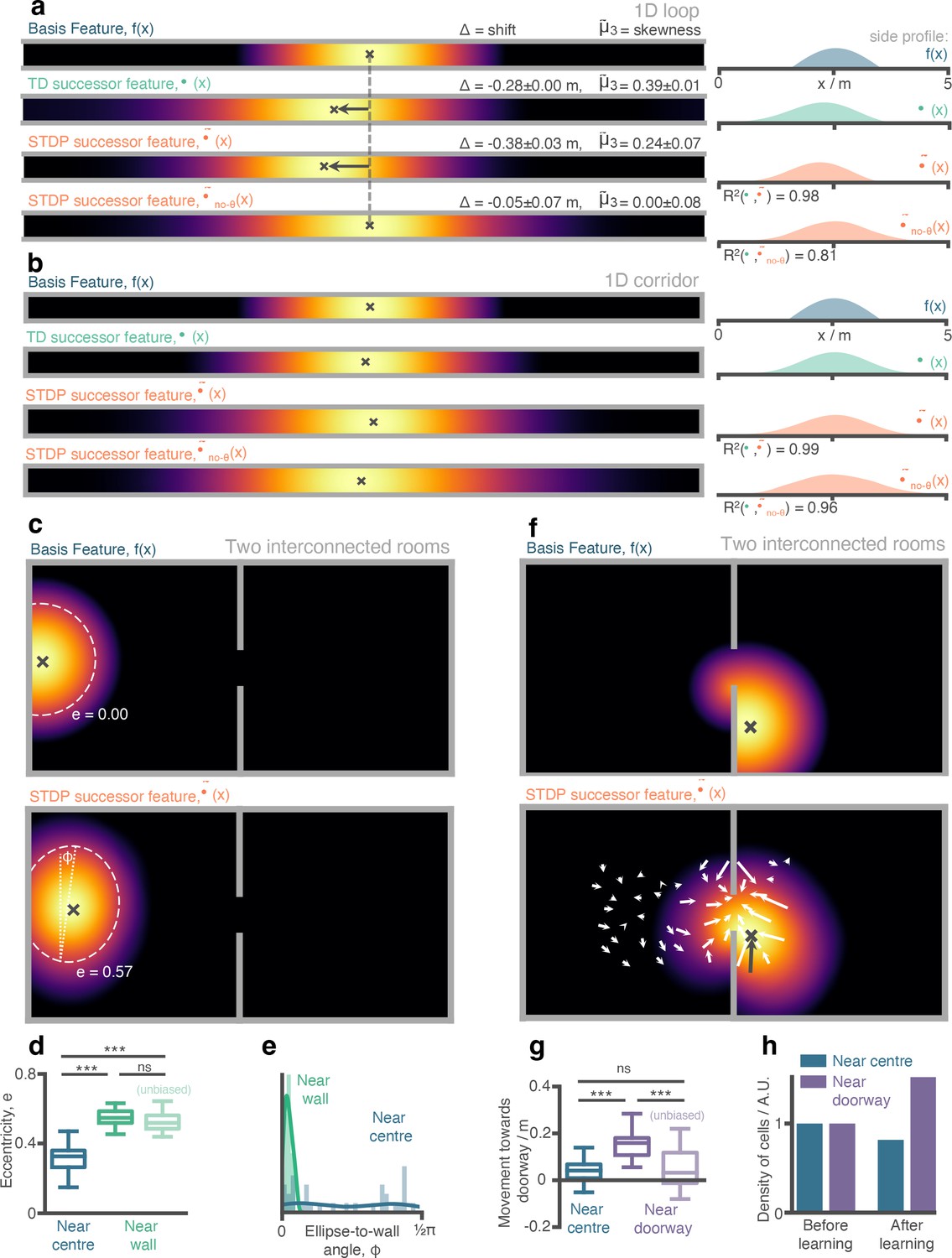
Place cells (aka. successor features) in our STDP model show behaviourally biased skewing resembling experimental observations and successor representation predictions.
(a) In the loop maze (motion left-to-right), STDP place cells skew and shift backwards, and strongly resemble place cells obtained via temporal difference learning. This is not the case when theta phase precession is absent. (b) In the corridor maze, where travel in either direction is equally likely, place fields defuse in both directions due to the unbiased movement policy. (c) In the 2D maze, place cells (of geodesic Gaussian basis features) near the wall elongate along the wall axis (dashed line shows best fitting ellipse, angle construct show the ellipse-to-wall angle). (d) Place cells near walls have higher elliptical eccentricity than those near the centre of the environments. This increase remains even when the movement policy bias to follow walls is absent. (e) The eccentricity for fields near the walls is facilitated by an increase in the length of the place field along an axis parallel to the wall ( close to zero). (f) Place cells near the doorway cluster towards it and expand through the doorway relative to their parent basis features. (g) The shift of place fields near the doorway towards the doorway is significant relative to place fields near the centre and disappears when the behavioural bias to cross doorways is absent. (h) The shift of place fields towards the doorway manifests as an increase in density of cells near the doorway after exploration.
Figure 4
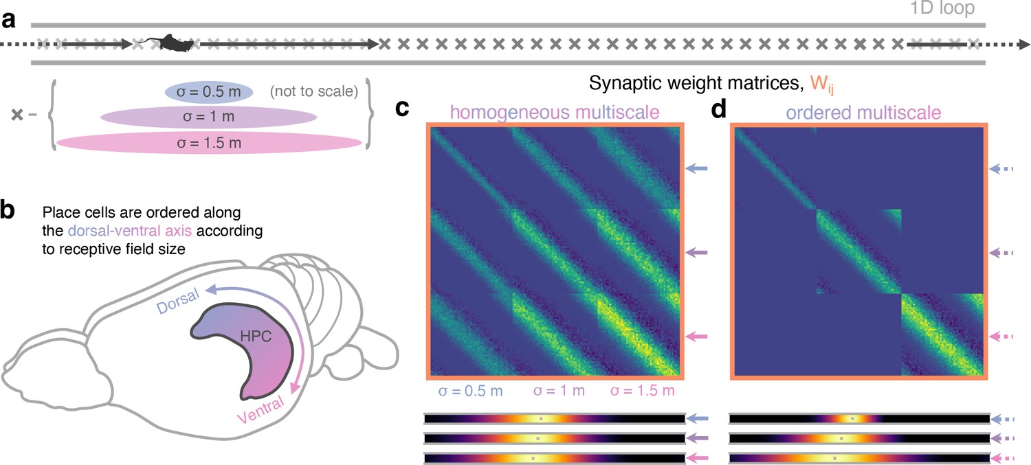
Multiscale successor representations are stored by place cells with multi-sized place fields but only when sizes are segregated along the dorso-ventral axis.
(a) An agent explores a 1D loop maze with 150 places cells of different sizes (50 small, 50 medium, and 50 large) evenly distributed along the track. (b) In rodent hippocampus, place cells are observed to be ordered along the dorso-ventral axis according to their field size. (c) When cells with different field sizes are homogeneously distributed throughout hippocampus all postsynaptic successor features can bind to all presynpatic basis features, regardless of their size (top). Short timescale successor representations are overwritten, creating three equivalent sets of redundantly large-scale successor features (bottom). (d) Ordering cells leads to anatomical segregation; postsynaptic successor features can only bind to basis features in the same size range (off-diagonal block elements are zero) preventing cells with different size fields from binding. Now, three dissimilar sets of successor features emerge with different length scales, corresponding to successor features of different discount time horizons.
Author response image 1

In a fully spiking model, CA1 neurons inherit phase precession from multiple upstream CA3 neurons.
Top, model schematic – each CA1 neuron receives input from multiple CA3 neurons with contiguous place fields. Bottom, position vs phase plot for an indicative CA1 neuron, showing strong phase precession similar to that observed in the brain.
Additional files
Download links
A two-part list of links to download the article, or parts of the article, in various formats.
Downloads (link to download the article as PDF)
Open citations (links to open the citations from this article in various online reference manager services)
Cite this article (links to download the citations from this article in formats compatible with various reference manager tools)
Rapid learning of predictive maps with STDP and theta phase precession
eLife 12:e80663.
https://doi.org/10.7554/eLife.80663


