Learning predictive cognitive maps with spiking neurons during behavior and replays
- Department of Bioengineering, Imperial College London, United Kingdom
Figures
Figure 1 with 2 supplements

Successor representation and neuronal network.
(A) Our simple example environment consists of a linear track with 4 states (S1 to S4) and the animal always moves from left to right — i.e. one epoch consists of starting in S1 and ending in S4. (B) The successor matrix corresponding to the task described in panel A. (C) Our neuronal network consists of a two layers with all-to-all feedforward connections. The presynaptic layer mimics hippocampal CA3 and the postsynaptic layer mimics CA1. (D) The synaptic plasticity rule consists of a depression term and a potentiation term. The depression term is dependent on the synaptic weight and presynaptic spikes (blue). The potentiation term depends on the timing between a pre- and post-synaptic spike pair (red), following an exponentially decaying plasticity window (bottom). (E–F) Schematics illustrating some of the results of our model. (E) Our spiking model learns the top row of the successor representation (panel B) in the weights between the first CA3 place cell and the CA1 cells. (F) Our spiking model learns the third row of successor representation (panel B) in the weights between the third CA3 place cell and the CA1 cells.
Figure 1—figure supplement 1
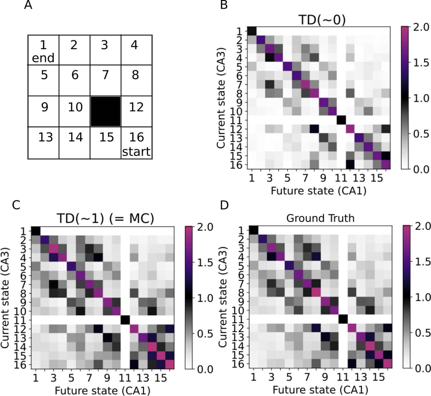
Learning the SR in a two-dimensional environment.
(A) Our two-dimensional environment contains 16 states. The 11th state is assumed to be an inaccessible obstacle. A random policy is guiding the trajectories, while the starting state is always state 16 and the trajectories only end when reaching state 1. (B–C) Successor representations learned by our model mimicking active exploration (TD(0)) and replays (TD(1)) respectively. (D) Ground truth successor representation.
Figure 1—figure supplement 2
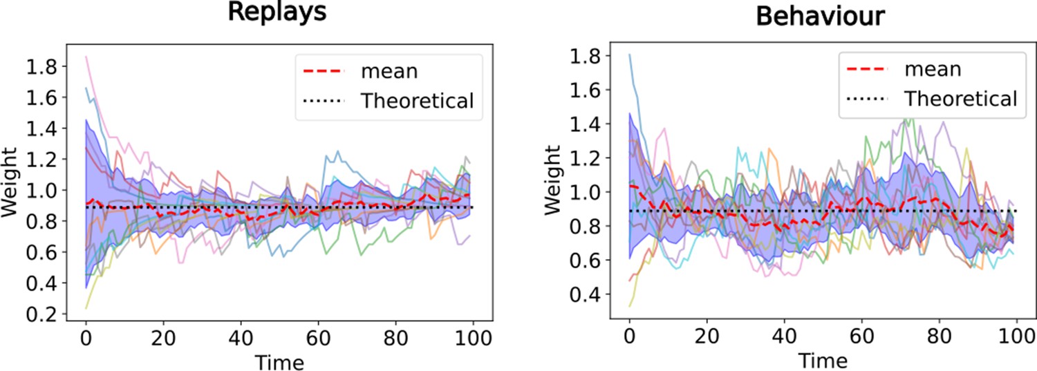
The equivalence with TD() guarantees convergence even with random initial synaptic weights.
Evolution of synaptic weights from CA3 state 2 to CA1 state 3 over time. Ten simulations of the linear track task (Figure 2) are performed, where the CA3-CA1 synaptic weights are randomly initialized at the start. The full lines denote the synaptic weight over time for each of the ten simulations, the red dashed line is the average over those and the black dotted line is theoretical value of the respective SR. In the left panel only replays are simulated (corresponding to TD ), in the right panel the behavioral model is simulated (corresponding to TD ).
Figure 2 with 1 supplement
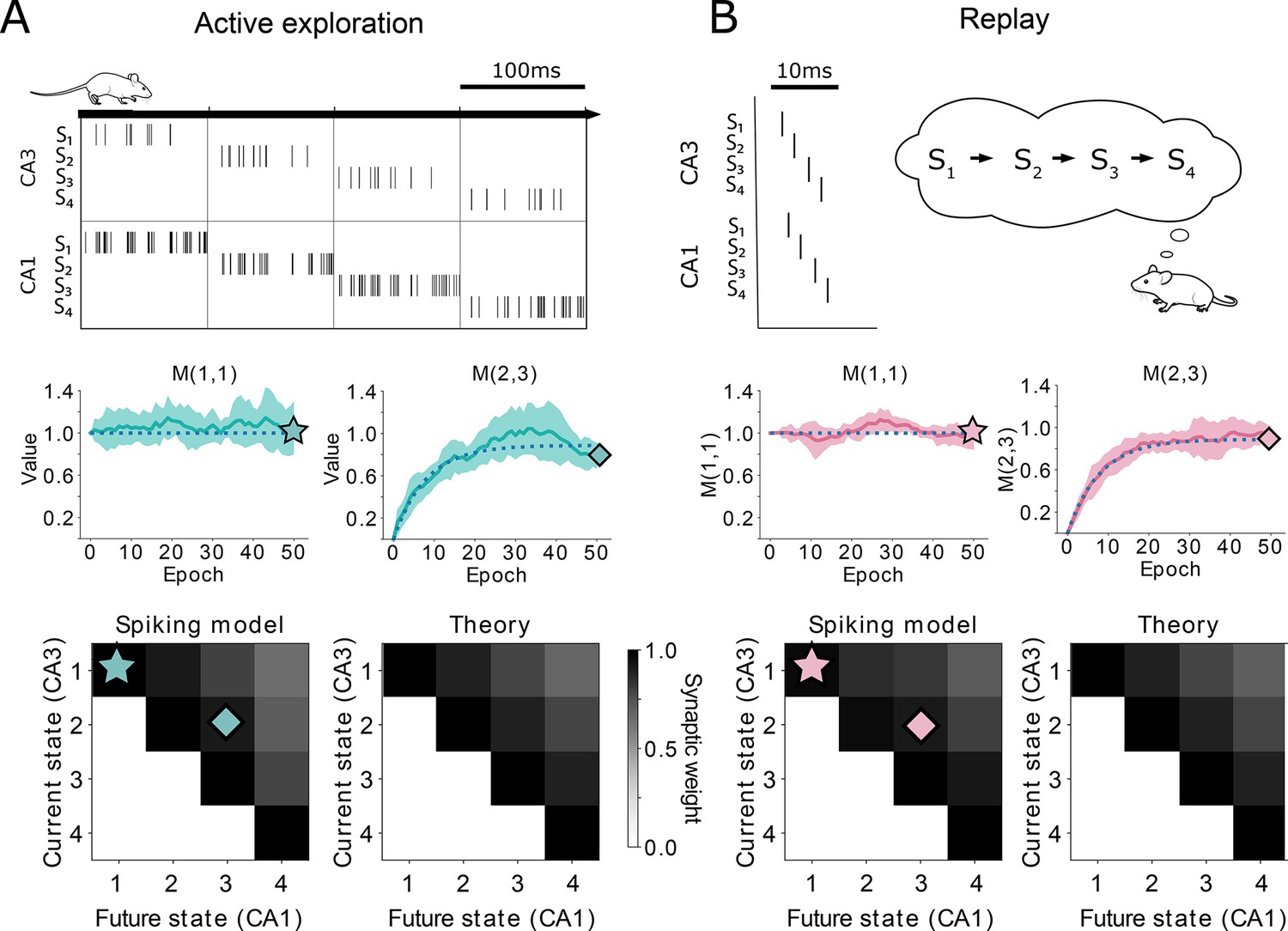
Comparison between TD() and our spiking model.
(A-top) Learning during behavior corresponds to TD(). States are traversed on timescales larger than the plasticity timescales and place cells use a rate-code. (A-middle) Comparison of the learning over epochs for two synaptic connections (full line denotes the mean over ten random seeds, shaded area denotes one standard deviation) with the theoretical learning curve of TD() (dotted line). (A-bottom) Final successor matrix learned by the spiking model (left) and the theoretical TD() algorithm (right). Star and diamond symbols denote the corresponding weights shown in the middle row. (B-top) Learning during replays corresponds to TD(). States are traversed on timescales similar to the plasticity timescales and place cells use a temporally precise code. (B-middle and bottom) Analogous to panel A middle and bottom.
Figure 2—figure supplement 1
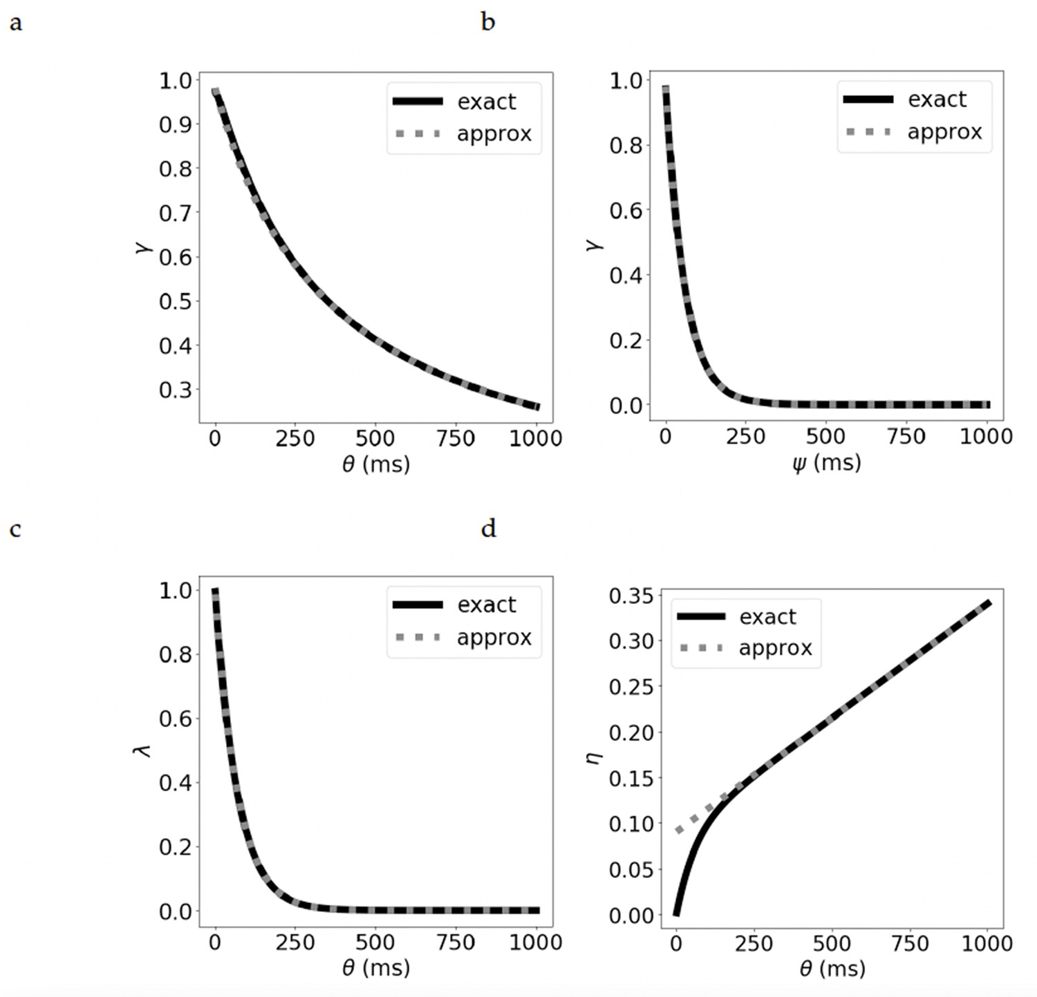
Comparison of the exact and approximate equations for the parameters.
The discount parameter when we vary by: (a) increasing the duration of the presynaptic current, leading to a hyperbolic discount, and (b) increasing , while keeping fixed, leading to an exponential discount. (c) The bootstrapping parameter for varying . (d) The learning rate for varying . See Supplementary materials for derivation of the exact and approximate equations.
Figure 3
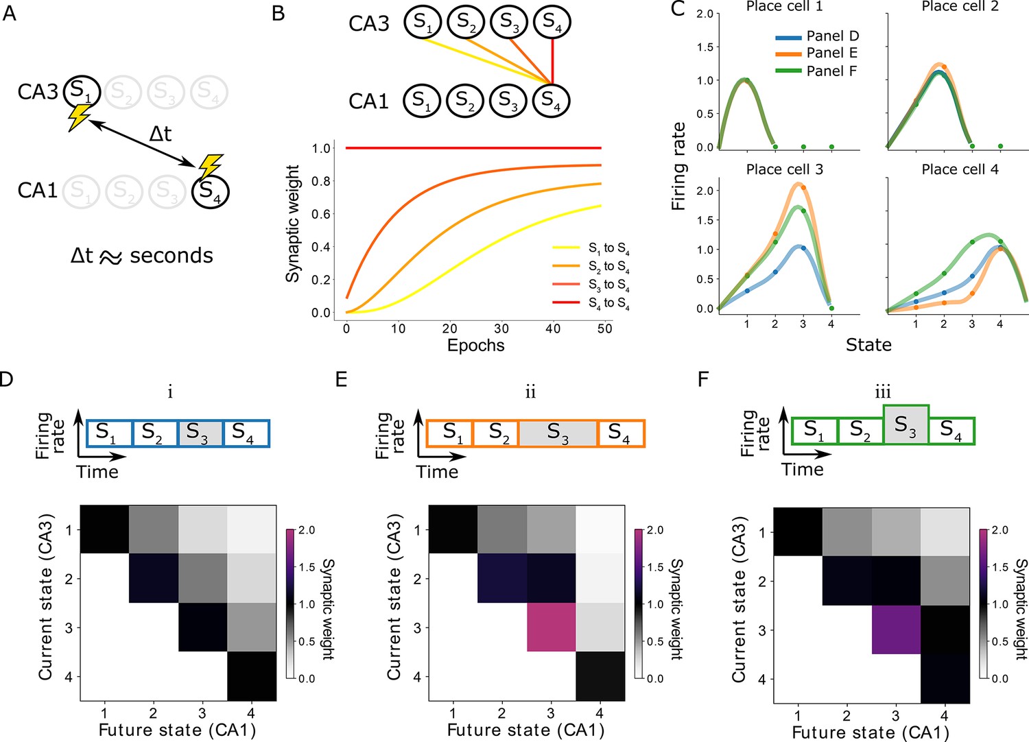
Learning on behavioral timescales and state-dependent discounting.
(A) In our model, the network can learn relationships between neurons that are active seconds apart, while the plasticity rule acts on a millisecond timescale. (B) Due to transitions between subsequent states, each synaptic weight update depends on the weight from the subsequent CA3 neuron to the same CA1 neuron. In other words, the change of a synaptic weight depends on the weight below it in the successor matrix. The top panel visualizes how weights depend on others in our linear track example, where each lighter color depends on the darker neighbor. The bottom panel shows the learning of over 50 epochs. Notice the lighter traces converge more slowly, due to their dependence on the darker traces. (C) Place fields of the place cells in the linear track — each place cell corresponding to a column of the successor matrix. Activities of each place cell when the animal is in each of the four states (dots) are interpolated (lines). Three variations are considered: (i) the time spent in each state and the CA3 firing rates are constant (blue and panel D); (ii) the time spent in state 3 is doubled (orange and panel E); (iii) the CA3 firing rate in state 3 is doubled (green and panel F). Panels E and F lead to a modified discount parameter in state 3, affecting the receptive fields of place cells 3 and 4.
Figure 4 with 2 supplements

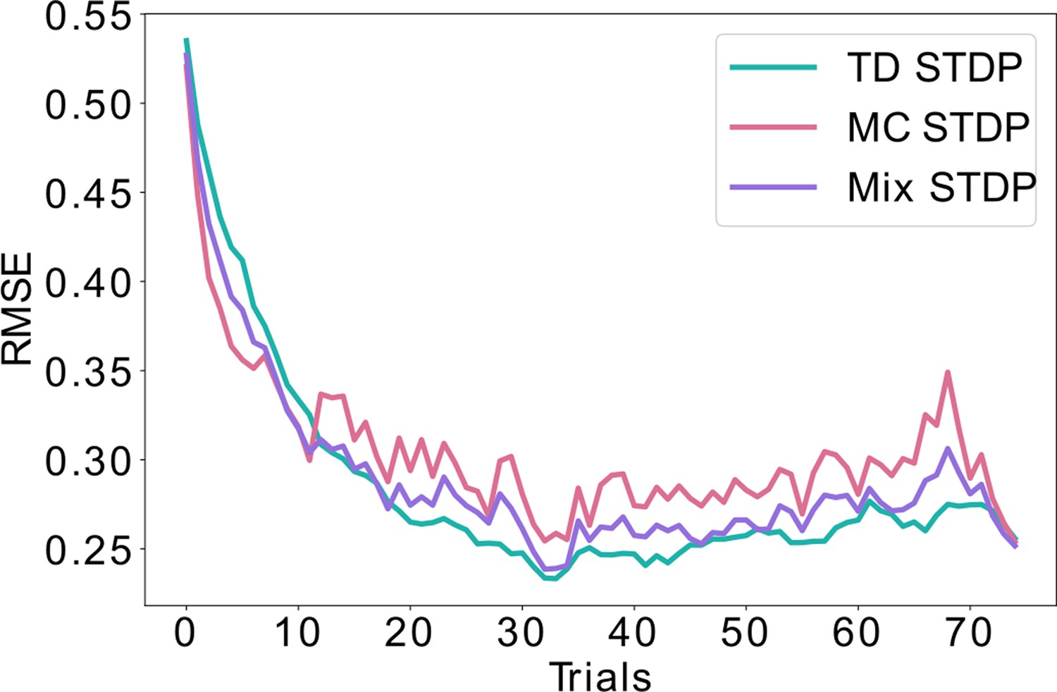
Replays can be used to control the bias-variance trade-off.
(A) The agent follows a stochastic policy starting from the initial state (denoted by START). The probability to move to either neighboring state is 50%. An epoch stops when reaching a terminal state (denoted with STOP). (B) Root mean squared error (RMSE) between the learned SR estimate and the theoretical SR matrix. The full lines are mean RMSEs over 1000 random seeds. Three cases are considered: (i) learning happens exclusively due to behavioral activity (TD STDP, green); (ii) learning happens exclusively due to replay activity (MC STDP, purple); (iii) A mixture of behavioral and replay learning, where the probabilities for replays drops off exponentially with epochs (Mix STDP, pink). The mix model, with a decaying number of replays learns as quickly as MC in the first epochs and converges to a low error similar to TD, benefiting both from the low bias of MC at the start and the low variance of TD at the end. (C, D, E) Representative weight changes for each of the scenarios. Full lines show various random seeds, shaded areas denote one standard deviation over 1000 random seeds. (F) More replays are observed when an animal explores a novel environment (day 1). Panel F adapted from Figure 3A in Cheng and Frank, 2008.
Figure 4—figure supplement 1
Combining equal amounts of replays and behavioral learning.
Unlike Figure 4, where the likelihood of replays is exponentially decaying over time, here we simulate equal probability for learning using replays (MC) and using behavioral experience (TD) throughout time. This mixed strategy lowers the bias and the variance to some extent, but lays between the pure MC and pure TD learning, never achieving the minimal error possible. This is in contrast with the exponential decay of replays shown in Figure 4, which achieves a minimal error both during early learning (similar to MC) as well as asymptotically (similar to TD).
Figure 4—figure supplement 2
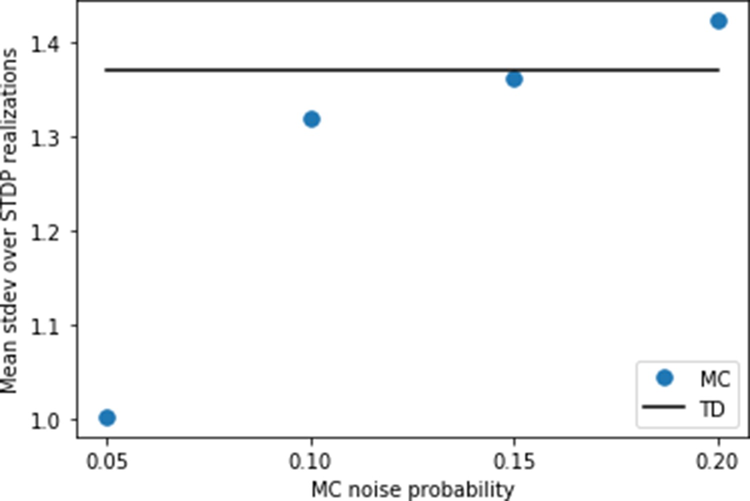
Setting the noise for replays.
Using the settings of Figure 4, we calculate the variance caused by random spiking for the behavioral model first. For this purpose, we simulate the same trajectory of the agent 25 times with different random instances of spikes generated from the Poisson process. At each state transition, we calculate the standard deviation of the synaptic weights over the 25 runs. Finally, we calculate the mean of these standard deviations over all states of the trajectory. We find a value of this mean standard deviation just below 1.4 (full line). Then, we try various levels of noise for the replay model, and compute the same mean standard deviation. We find that a probability yields a similar level of variance due to random spiking as in the behavioral model.
Figure 5 with 4 supplements
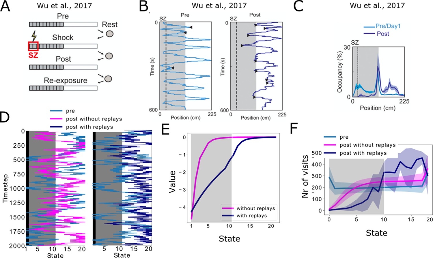
Reproducing place-avoidence experiments with the spiking model.
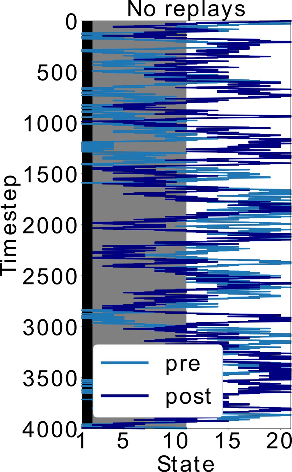
(A–C) Data from Wu et al., 2017. (A) Experimental protocol: the animal is first allowed to freely run in the track (Pre). In the next trial, a footshock is given in the shock zone (SZ). In subsequent trials the animal is again free to run in the track (Post, Re-exposure). Figure redrawn from Wu et al., 2017. (B) In the Post trial, the animal learned to avoid the shock zone completely and the also mostly avoids the dark area of the track. Figure redrawn from Wu et al., 2017. (C) Time spent per location confirms that the animal prefers the light part of the track in the Post trial. Figure redrawn from Wu et al., 2017. (D) Mimicking the results from Wu et al., 2017, the shock zone is indicated by the black region, the dark zone by the gray region and the light zone by the white region. Left: without replays, the agent keeps extensively exploring the dark zone even after having experienced the shock. Right: with replays, the agent largely avoids entering the dark zone after having experienced the shock (replays not shown). (E) The value of each state in the cases with and without replays. (F) Occupancy of each state in our simulations and for the various trials. Solid line and shaded areas denote the average and standard deviation over 100 simulations, respectively. Notice we do not reproduce the peak of occupancy at the middle of the track as seen in panel c, since our simplified model assumes the same amount of time is spent in each state.
Figure 5—figure supplement 1
Doubling the time-steps in the scenario without replays.
In Figure 5, the policy without replays has less SR updates. Here, we simulated this policy but doubled the time (and SR updates). Even with this modification, the agent keeps exploring the dark zone of the track, which shows that it is indeed the type of policy and not the amount of updates that leads to the different behavior. More specifically, sequential activations of states from the decision point until the shock zone, such as in replays, are different than the softmax policy during behavior. It is exactly by exploiting this different replay policy that the agent updates the SR differently and avoids the dark zone.
Figure 5—figure supplement 2
The value of states can be read out by downstream neurons.
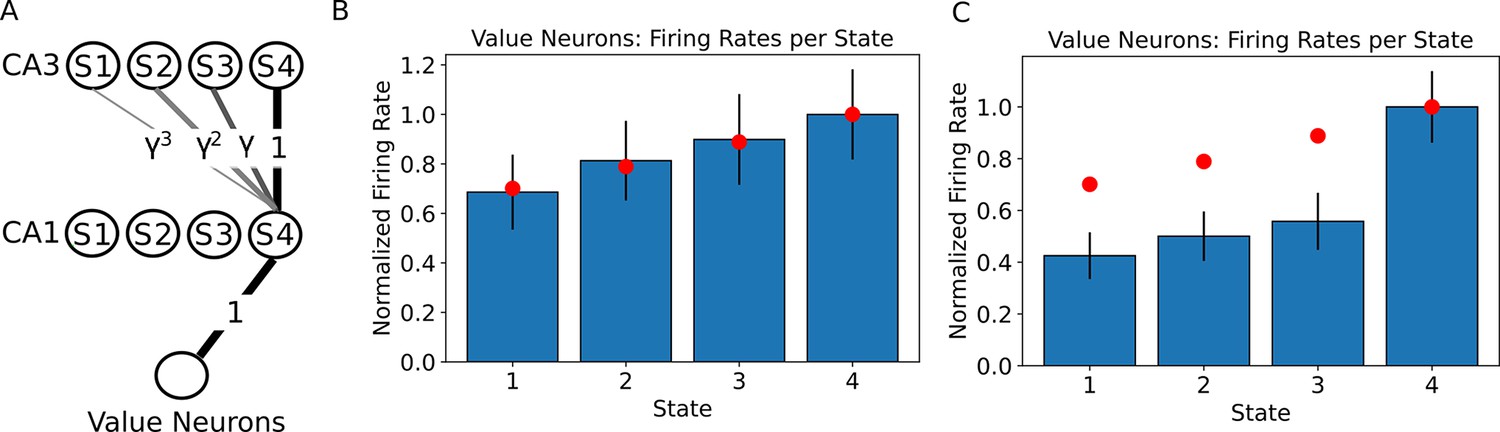
(A) A linear track with 4 states is simulated as in Figure 1, where we now assume the state 4 contains a reward with value 1. This reward is assumed to be encoded in the synaptic weights from the CA1 neurons to the value neurons. We simulated a population of 250 neurons encoding each state and 250 neurons encoding the value. (B) Firing rates of the value neurons when the agent is occupying each state of the linear track. Only the firing rates during the first 80% of the dwelling time are shown, since no external input is applied during that time. Bars denote the mean firing rate of the 250 value neurons, error bars denote one standard deviation. Red dots denote the ground truth value for each state. (C) When the firing rates of the value neurons are computed over the full dwelling time in each state, the estimate of the value changes qualitatively due to the external input to CA1 in the final fraction of the dwelling time. Bars denote the mean firing rate of the 250 value neurons, error bars denote one standard deviation. Red dots denote the ground truth value for each state. Note that the ranking of the states by value is not affected. Practically, using the parameters in our simulation, one could either read out the correct estimate of the value during the first 80% of the dwelling time in a state, or learn a correction to this perturbation in the weights to the value neuron, or simply use a policy that is based on the ranking of the values instead of the actual firing rate.
Figure 5—figure supplement 3
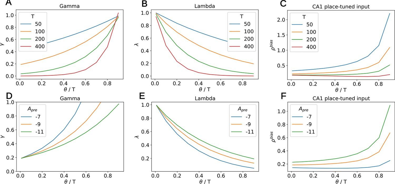
Dependency of , and the place-tuned input to CA1 on , for various values of T and depression amplitude .
(A) The variable increases with the ratio and decreases with T. (B) The variable decreases with the ratio and decreases with T. (C) The input to CA1 increases with the ratio. Therefore, the longer this input lasts (i.e. the lower ), the smaller it is. The distortion of the diagonal elements of the SR thus remains similar across various. For high values of T, the input remains more or less constant at low values. (D) The variable decreases with the depression amplitude and decreases with T. For fixed , one can choose any by tuning this amplitude. (E) The variable increases with the depression amplitude . (F) The input to CA1 increases with the depression amplitude . For fixed , this implies that stronger inputs are coupled with higher and therefore shorter duration. The distortion of the diagonal elements of the SR thus remains similar across various .
Figure 5—figure supplement 4
Readout of the state value for various parameters.
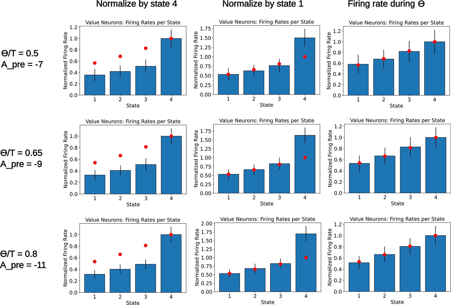
A population of readout neurons is simulated as in Figure 5—figure supplement 2. Each row corresponds to a different choice of parameters and , chosen such that the variable has a value close to 0.815. The rate of the readout neurons is computed when the agent occupies the various states. Rates are either normalized by the final state (left column) or the initial state (middle column). The right column denotes a computation of the firing rate of the readout neurons during the initial part of the dwelling time, . As in Figure 5—figure supplement 2, bars denote the mean firing rate of the 250 value neurons, error bars denote one standard deviation. Red dots denote the ground truth value for each state. We notice that, for various values of , the deviation from the ground truth remains similar. Furthermore, since the deviation is only affecting the diagonal elements of the SR with a fixed amount determined by and , some compensatory mechanism could be easily incorporated in the network.
Tables
Table 1
Parameters used for the spiking network.
| 1 | |
| 0.1ms-1 | |
| 2ms | |
| 1 | |
| 1 | |
| 1 | |
| stepsize | 0.01ms |
| 0.003 | |
| 60ms | |
| 1 ms-1 |
Additional files
Download links
A two-part list of links to download the article, or parts of the article, in various formats.
Downloads (link to download the article as PDF)
Open citations (links to open the citations from this article in various online reference manager services)
Cite this article (links to download the citations from this article in formats compatible with various reference manager tools)
Learning predictive cognitive maps with spiking neurons during behavior and replays
eLife 12:e80671.
https://doi.org/10.7554/eLife.80671


