Figures and data in Sweepstakes reproductive success via pervasive and recurrent selective sweeps

Figures
Tables
Additional files

28 figures, 10 tables and 1 additional file

Figures

Figure 1 with 2 supplements

Download asset Open asset

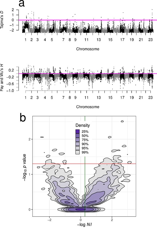
Neutrality test statistics and distribution of the neutrality index.

(a) Manhattan plots of Tajima’s D (Tajima, 1989) and Fay and Wu's $H$ (Fay and Wu, 2000) showed mostly negative values at all chromosomes implying deviations from neutrality. Sliding window estimates (window size 100 kb with 20 kb step size) using GL1 genotype likelihoods for the South/south-east population. Value of the statistic under Kingman coalescent neutrality equilibrium indicated with magenta horizontal line. (b) Kernel density contours (Duong, 2022) of the $- \log_{10} p$ value significance of Fisher’s exact test associated with the McDonald–Kreitman test (McDonald and Kreitman, 1991) plotted against the neutrality index (Rand and Kann, 1996) $- \log N I N I = (P_{n} \times D_{s}) / (P_{s} \times D_{n})$ . $N I = (P_{n} / P_{s}) / (D_{n} / D_{s})$ where $P_{n}$ , $P_{s}$ , $D_{n}$ , and $D_{s}$ are the number of non-synonymous and synonymous polymorphic and fixed sites, respectively, for all genes of each chromosome. Negative values of $- \log N I$ imply purifying (negative) and background selection and positive values imply positive selection (selective sweeps). The outgroup is Pacific cod (Gma). Overall, the cloud of positive values is denser than the cloud of negative values. The red horizontal line is at nominal significance level of 0.05 for individual tests; no test reached the $0.05 / n$ Bonferroni adjustment for multiple testing. The mean (green vertical line) and the median of $- \log N I$ were 0.27 and 0.21, respectively, and imply that the proportion of adaptive non-synonymous substitutions $α = 1 - N I$ (Smith and Eyre-Walker, 2002) is 19–24%. Figure 1—figure supplement 1 shows neutrality statistics for the Þistilfjörður population. Figure 1—figure supplement 2 shows distribution and violin plot of $- \log N I$ across each chromosome from the South/south-east population.

Figure 1—figure supplement 1

Download asset Open asset

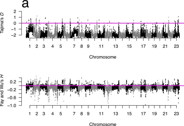
Neutrality tests for Þistilfjörður population.

(a) Manhattan plots of Tajima’s D (Tajima, 1989) and Fay and Wu's $H$ (Fay and Wu, 2000) for the Þistilfjörður population showed mostly negative values at all chromosomes implying deviations from neutrality. Sliding window estimates (window size 100 kb with 20 kb step size) using GL1 genotype likelihoods. Value of statistic under Kingman coalescent neutrality equilibrium indicated with magenta horizontal line.

Figure 1—figure supplement 2

Download asset Open asset

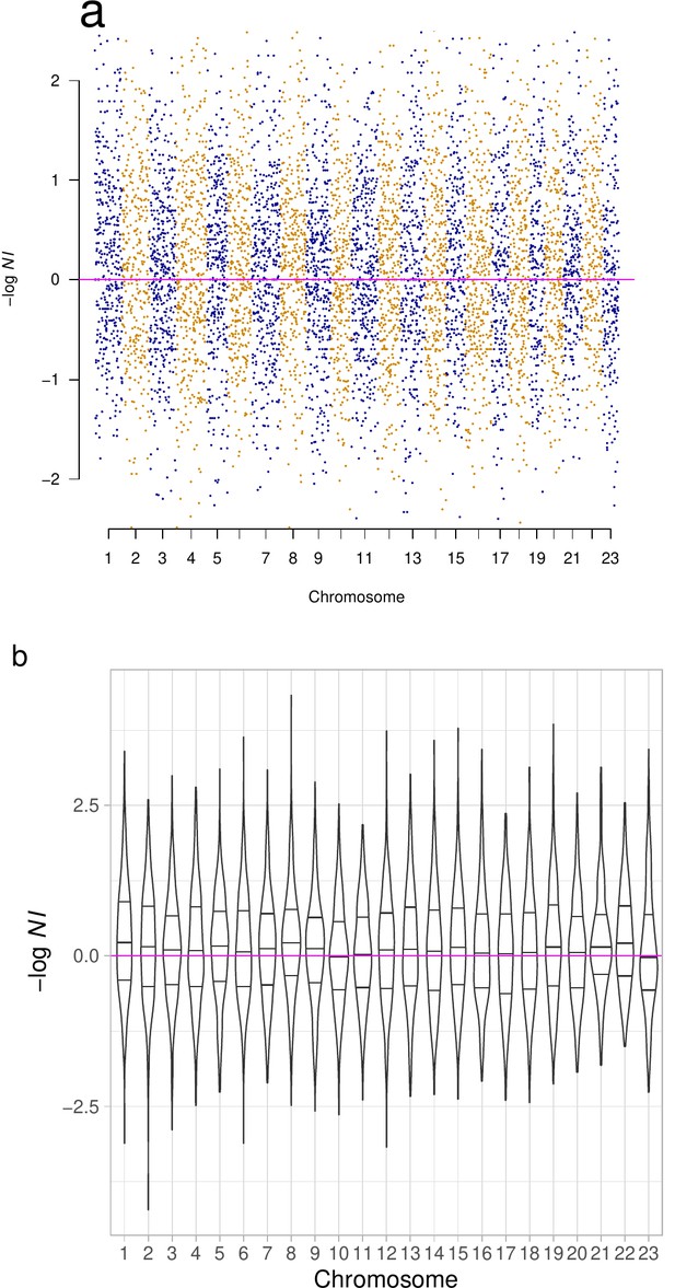
Neutrality Index and violin plot of neutrality index across chromosomes.

(a) The distribution of $- \log N I$ (neutrality index) per chromosome (and (b) violin plots with quartiles) were heavier on the positive side implying more positive than negative selection.

Figure 2 with 1 supplement

Download asset Open asset

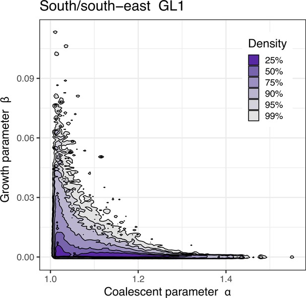
Approximate Bayesian computation (ABC) joint estimation of parameters of the neutral $Ξ$ -Beta( $2 - α, α$ ) coalescent (random sweepstakes) and of population growth.

A kernel density estimator (Duong, 2022) for the joint ABC-posterior density of $(α, β) \in Θ_{B}$ . The parameter $α$ determines the skewness of the offspring distribution in the neutral $Ξ$ -Beta( $2 - α, α$ ) coalescent model, and the parameter $β$ is a population-size rescaled rate of exponential population growth. Estimates using GL1 for the South/south-east population. A bivariate model-fitting analysis adding exponential population growth to the $Ξ$ -Beta( $2 - α, α$ ) coalescent does not improve model fit for random sweepstakes. The population growth parameter ( $β$ ) only has an effect under maximal sweepstakes (low values of $α$ ). Figure 2—figure supplement 1 explores the random sweepstakes model with population growth using both GL1 and GL2 likelihood estimates of site-frequency spectra for both the South/south-east and Þistilfjörður populations, and for different ranges of parameter values.

Figure 2—figure supplement 1

Download asset Open asset

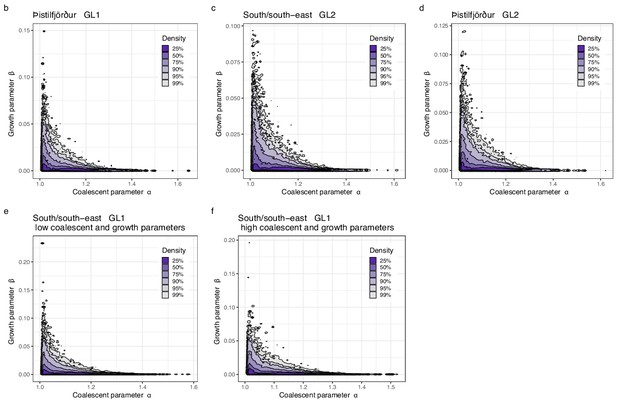
Joint estimate of growth and coalescent parameter for other situations.

Approximate Bayesian computation (ABC) joint estimation of parameters of the neutral $Ξ$ -Beta( $2 - α, α$ ) coalescent (random sweepstakes) and of population growth. A kernel density estimator for the joint ABC-posterior density of $(α, β) \in Θ_{B}$ . The parameter $α$ determines the skewness of the offspring distribution in the neutral Beta( $2 - α, α$ ) coalescent model, and the $β$ is a population-size rescaled rate of exponential population growth. (b) Estimates using GL1 for the Þistilfjörður population, (c) using GL2 for the South/south-east population, (d) using GL2 for the the Þistilfjörður population, and using GL1 for the South/south-east population with a narrower (e) and a wider (f) range of parameter values.

Figure 3 with 4 supplements

Download asset Open asset

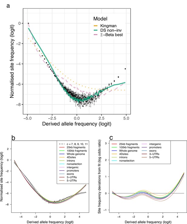
Fit of observations to models: the no-sweepstakes model, the random sweepstakes model, and the selective sweepstakes model.

(a) Mean observed site-frequency spectra for the 19 non-inversion chromosomes combined estimated with GL1 likelihood for the South/south-east populations (sample size $n = 68$ ). Error bars of observed data (dots) are ±2 standard deviations of the bootstrap distribution with 100 bootstrap replicates. Expected site-frequency spectra are the Kingman coalescent modelling no sweepstakes, the best approximate maximum likelihood estimates (Eldon et al., 2015) of the $Ξ$ -Beta coalescent modelling random sweepstakes, and the approximate Bayesian computation (ABC) estimated Durrett–Schweinsberg coalescent (DS) modelling selective sweepstakes. (b) The observed site-frequency spectra of different sized fragments and various functional classes compared to expectations of the Durrett–Schweinsberg coalescent (DS) ABC estimated for the non-inversion chromosomes for the South/south-east population. The compound parameter $c$ ranges from 5 to 11. Fragment sizes of 25 and 100 kb. The different functional groups are fourfold degenerate sites (4Dsites), intronic sites, non-selection sites (sites more than 500 kb away from peaks of selection scan, Appendix 6—figure 8), intergenic sites, promoters, exons, $3^{'}$ -UTR sites (3-UTRs), and $5^{'}$ -UTR sites (5-UTRs) in order of selective constraints. (c) Deviations from expectations of the Durrett–Schweinsberg model of recurrent selective sweeps of different sized fragments and functional groups for the South/south-east population. Figure 3—figure supplement 1 shows comparable results for the Þistilfjörður population. Figure 3—figure supplement 1 shows site-frequency spectrum polarized with 100% consensus of walleye pollock (Gch), Pacific cod (Gma), and Arctic cod (Bsa) to minimize potential effects of SNP misorientation and low-level ancestral introgression (Appendix 10). Figure 3—figure supplement 4 shows site-frequency spectrum for transversions only removing transition sites that are more likely to be at mutation saturation to adddress potential SNP misorientation. Figure 3—figure supplement 4 shows site-frequency spectrum truncated by removing singletons and doubletons and the $n - 1$ and $n - 2$ classes that are most sensitive to SNP misorientation and low-level ancestral introgression.

Figure 3—figure supplement 1

Download asset Open asset

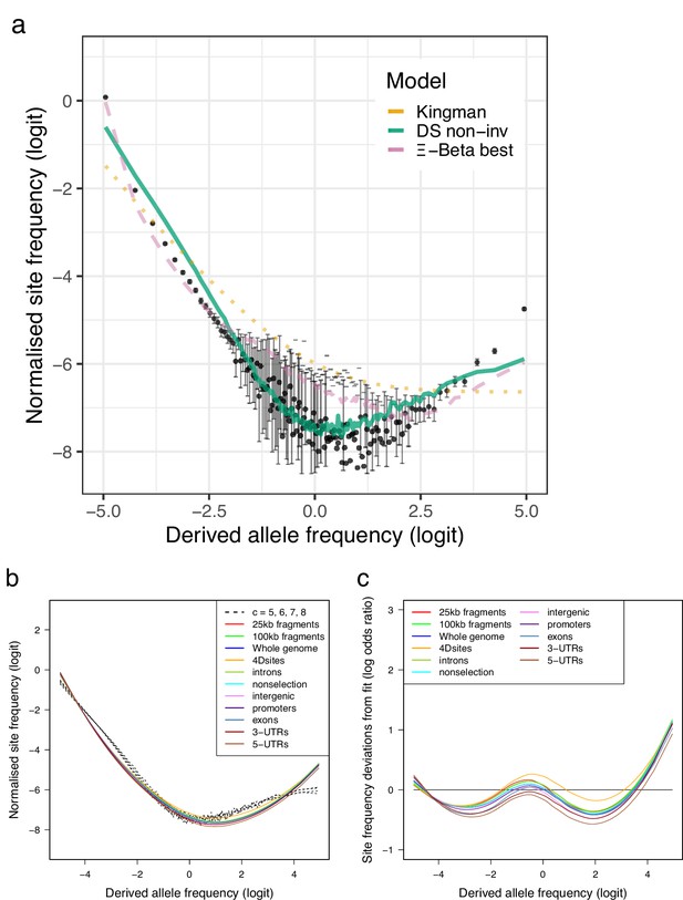
Site-frequency spectra and model fit for the replicate Þistilfjörður population.

(a) Site-frequency spectra of 19 non-inversion chromosomes compared to expectations of Kingman-, $Ξ$ -Beta-, and Durrett–Schweinsberg (DS) coalescents for the Þistilfjörður population (sample size $n = 71$ ). Error bars of observed data (dots) are ±2 standard deviations of the bootstrap distribution with 100 bootstrap replicates. (b) Site-frequency spectra of random fragments and various functional groups compared to expecations of the DS coalescent for the compound parameter $c$ ranging from 5 to 8. (c) Deviations from DS expectations for random fragments and various functional groups.

Figure 3—figure supplement 2

Download asset Open asset

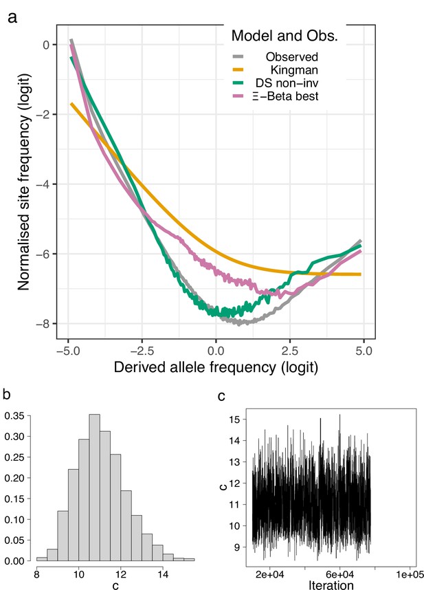
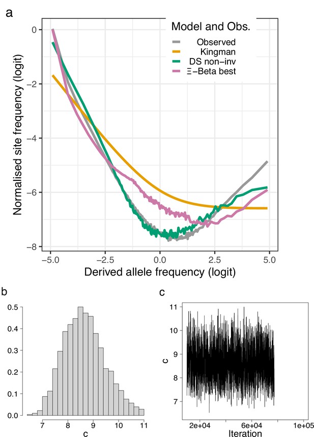
Site-frequency spectra polarized using a 100% consensus of three outgroup taxa.

(a) Site-frequency spectra otained using as outgroup sites that are in full agreement (100% consensus) among walleye pollock (Gch), Pacific cod (Gma), and Arctic cod (Bsa) compared with expectations of the Kingman, the $Ξ$ -Beta, and the Durrett–Schweinsberg coalescents (a). The distribution (b) and traces (c) of the approximate Bayesian computation (ABC) estimation of the compound parameter $c$ of the Durrett–Schweinsberg coalescent. Based on observed data of the 19 non-inversion chromosomes combined for the South/south-east population (sample size $n = 68$ ).

Figure 3—figure supplement 3

Download asset Open asset

Site-frequency spectra of transversions excluding transitions.

Site-frequency spectra and model fit of transversions of the 19 non-inversion chromosomes of the South/south-east population compared with expectations of of the Kingman, the $Ξ$ -Beta, and the Durrett–Schweinsberg colaescents (a). The distribution and traces of the approximate Bayesian computation (ABC) estimation of the compound parameter $c$ of the Durrett–Schweinsberg colaescent (**b, c**). Based on observed data of the 19 non-inversion chromosomes combined for the South/south-east population.

Figure 3—figure supplement 4

Download asset Open asset

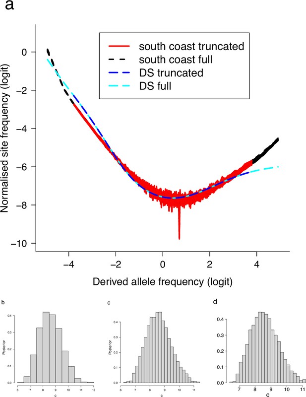
Site-frequency spectra excluding singletons and doubletons.

(a) Truncated and full site-frequency spectra compared. Singleton and the $n - 1$ class and doubleton and the $n - 2$ class were excluded and compared with the full site-frequency spectrum and with expectations of the Durrett–Schweinsberg colaescent (DS). (b) The distribution of the approximate Bayesian computation (ABC) estimation of the compound parameter $c$ of the Durrett–Schweinsberg colaescent excluding singletons and $n - 1$ class, (c) also excluding doubletons and the $n - 2$ class, and (d) the distribution for the full data. Based on observed data of the 19 non-inversion chromosomes combined for the South/south-east population.

Figure 4 with 1 supplement

Download asset Open asset

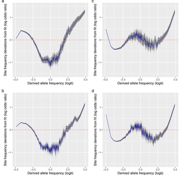
Deviations from fit to the random sweepstakes model and the selective sweepstakes model.

(**a, b**) Deviations of site frequencies from approximate maximum likelihood best-fit expectations of the neutral $Ξ$ -Beta( $2 - α, α$ ) coalescent modelling random sweepstakes. Deviations of the mean site frequencies of non-inversion chromosomes 3–6, 8–11, and 13–23 estimated with genotype likelihoods GL1 from best-fit expectations of the $Ξ$ -Beta( $2 - α, α$ ) coalescent with $\hat{α} = 1.16$ for the South/south-east population (sample size $n = 68$ ) (a) and with $\hat{α} = 1.16$ for the Þistilfjörður population (sample size $n = 71$ ) (b). Deficiency of intermediate allele frequency classes and excess mainly at right tail of site-frequency spectrum. (**c, d**) Deviations of GL1 estimated site frequencies from expectations of the Durrett–Schweinsberg model of recurrent selective sweeps for the South/south-east population with a compound parameter $c = 8.25$ and the Þistilfjörður population with a compound parameter $c = 6.3$ , respectively. Better fit than random model but also with excess at right tail of site-frequency spectrum. Deviations reported as the log of the odds ratio (in blue), the difference of the observed and expected logit of site frequencies. The dashed red line at zero represents the null hypothesis of no difference between observed and expected. The darker and lighter shaded gray areas represent the 95% and the 99% confidence regions of the approximately normally distributed log odds ratio. Figure 4—figure supplement 1 shows comparable deviation from fit for the GL2 genotype likelihood data.

Figure 4—figure supplement 1

Download asset Open asset

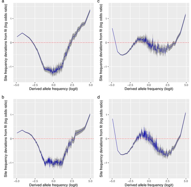
Deviations from fit to the random sweepstakes model and the selective sweepstakes model for GL2 genotype likelihood data.

(**a, b**) Deviations of the mean site frequencies of non-inversion chromosomes 3–6, 8–11, and 13–23 estimated with genotype likelihoods GL2 from approximate maximum likelihood best-fit expectations of the neutral $Ξ$ -Beta( $2 - α, α$ ) coalescent (random sweepstakes model) for the South/south-east population with $\hat{α} = 1.04$ and for the Þistilfjörður population with $\hat{α} = 1.12$ , respectively. (**c, d**) Deviations of the mean site frequencies of non-inversion chromosomes 3–6, 8–11, and 13–23 estimated with genotype likelihoods GL2 from expectations of the Durrett–Schweinsberg model of recurrent selective sweeps for the South/south-east population with a compound parameter $\hat{c} = 10.75$ and the Þistilfjörður population with a compound parameter $\hat{c} = 9.25$ , respectively. Deviations reported as the log of the odds ratio (in blue), the difference of the observed and expected logit of site frequencies. The dashed red line at zero represents the null hypothesis of no difference between observed and expected. The darker and lighter shaded gray areas represent the 95% and the 99% confidence regions of the approximately normally distributed log odds ratio. Samples sizes $n = 68$ and $n = 71$ for the South/south-east and Þistilfjðröur populations respectively.

Figure 5

Download asset Open asset

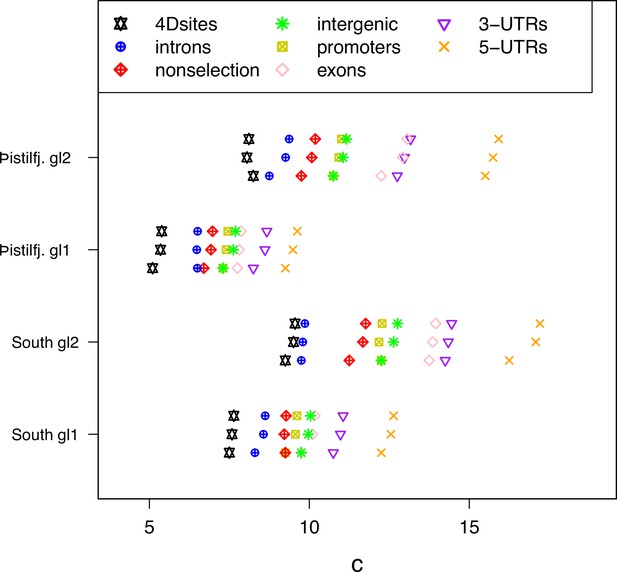
Approximate Bayesian computation (ABC) estimation of parameters of the Durrett-Schweinsberg coalescent (Durrett and Schweinsberg, 2005) (the selective sweepstakes model) for various functional regions of the genome.

For each category from top to bottom the mean, the median, and the mode of the ABC-posterior distribution of the compound parameter $c \in Θ_{DS}$ using site-frequency spectra computed from likelihood GL1 and GL2 for the South/south-east (South) and Þistilfjörður (Þistilfj.) populations. The different functional groups are fourfold degenerate sites (4Dsites), intronic sites, non-selection sites (sites more than 500 kb away from peaks of selection scan, Appendix 6—figure 8), intergenic sites, promoters, exons, $3^{'}$ -UTR sites (3-UTRs), and $5^{'}$ -UTR sites (5-UTRs), regions ranging from less to more constrained by selection.

Figure 6

Download asset Open asset

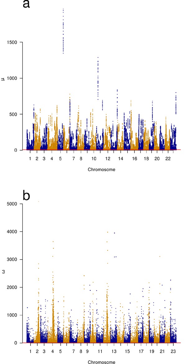
Genomic scans of selective sweeps by two methods.

(a) Manhattan plots from detection of selective sweeps using RAiSD (Alachiotis and Pavlidis, 2018) and (b) by using OmegaPlus (Alachiotis et al., 2012). The ω statistic of OmegaPlus (b) measures increased linkage disequilibrium in segments on either the left or the right sides of a window around selected site and a decrease in linkage disequilibrium between the segments across the selected site (Kim and Nielsen, 2004; Alachiotis and Pavlidis, 2018). The μ statistic of RAiSD (a) is a composite measure based on three factors, a reduction of genetic variation in a region around a sweep, a shift in the site-frequency spectrum from intermediate- towards low- and high-frequency derived variants, and a factor similar to ω that measures linkage disequilibrium on either side of and across the site of a sweep. Chromosomes with alternating colours. Indications of selective sweeps are found throughout each chromosome.

Appendix 6—figure 1

Download asset Open asset

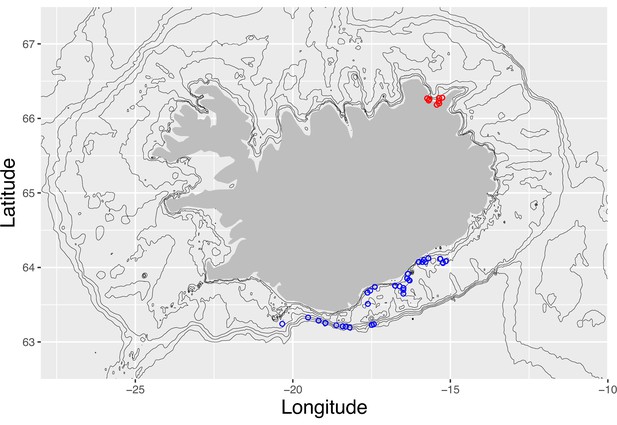
Sampling localities at Iceland.

Sampling localities ranging from Vestmannaeyjar to Höfn on the south and south-east coast (blue circles, $n = 68$ ) and Þistilfjörður in the north-east (red circles, $n = 71$ ) on a map of Iceland. Depth contours are at −25, −50, −100, −200, −400, −600, and −800 m. The two localities serve as statistical replicates, the South/south-east and the Þistilfjörður population, respectively.

Appendix 6—figure 2

Download asset Open asset

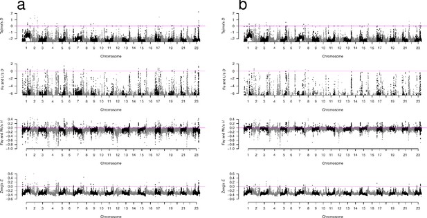
Neutrality test statistics in sliding windows across all chromosomes for GL2 estimates.

(**a, b**) Manhattan plots of Tajima’s D (Tajima, 1989), Fu and Li’s D (Fu and Li, 1993), Fay and Wu’s H (Fay and Wu, 2000), and Zeng’s E (Zeng et al., 2006) for the South/south-east population and the Þistilfjörður population, respectively. Sliding window estimates (window size 100 kb with 20 kb step size) using GL2 genotype likelihoods. Value of statistic under Kingman coalescent neutrality equilibrium indicated with magenta horizontal line.

Appendix 6—figure 3

Download asset Open asset

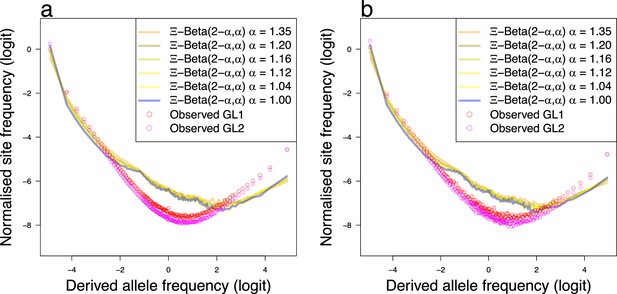
The random sweepstakes model.

(**a, b**) Observed site-frequency spectra of non-inversion chromosomes and expectations of the $Ξ$ -Beta( $2 - α, α$ ) coalescent (the random sweepstakes model) for the South/south-east population (sample size $n = 68$ ) and Þistilfjörður population (sample size $n = 71$ ), respectively. The observed mean site-frequency spectrum of the non-inversion chromosomes 3–6, 8–11, and 13–23 polarized with Gma as outgroup and estimated under genotype likelihoods GL1 and GL2 and expected site-frequency spectrum of the $Ξ$ -Beta( $2 - α$ , $α$ ) coalescent with $α = 1.35$ , $α = 1.20$ , $α = 1.16$ , $α = 1.12$ , $α = 1.04$ , and $α = 1.00$ which are representative samples of the posterior estimates that coincide with the kernel density estimates (Figure 2). The $α = 1.16$ , $α = 1.12$ , and $α = 1.04$ , which represent the approximate maximum likelihood best estimates as detailed in Figure 4a, b and Figure 4—figure supplement 1a, b.

Appendix 6—figure 4

Download asset Open asset

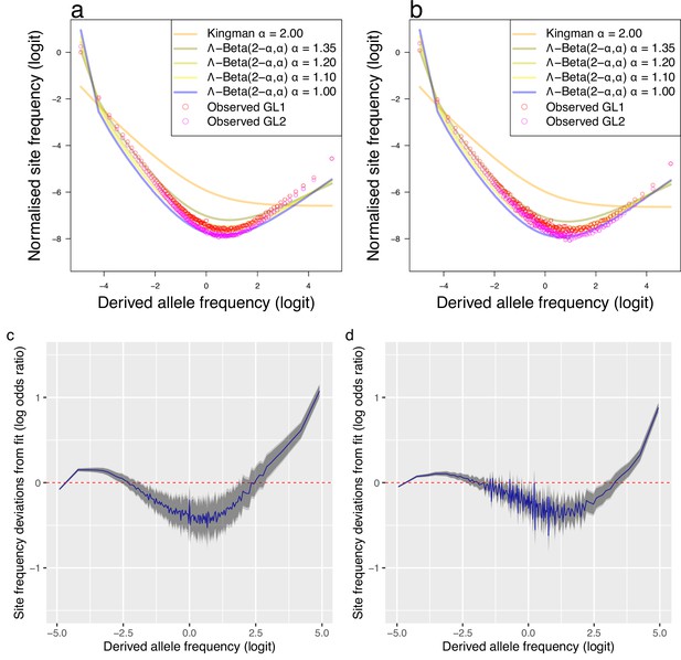
Piecewise comparison of expectations of the $Λ$ -Beta( $2 - α, α$ ) coalescent and deviations from fit.

The observed mean site-frequency spectrum of the non-inversion chromosomes 3–6, 8–11, and 13–23 polarized with Gma as outgroup and estimated under genotype likelihoods GL1 and GL2 and expected site-frequency spectrum of the $Λ$ -Beta( $2 - α, α$ ) coalescent with $α = 1.35$ , $α = 1.20$ , $α = 1.10$ , and $α = 1.00$ . Population South/south-east (sample size $n = 68$ ) (a) and population Þistilfjörður (sample size $n = 71$ ) (b). Deviations from the maximum likelihood estimated expecations of $Λ$ -Beta( $2 - α, α$ ) coalescent for the South/south-east (c) and the Þistilfjörður population (d).

Appendix 6—figure 5

Download asset Open asset

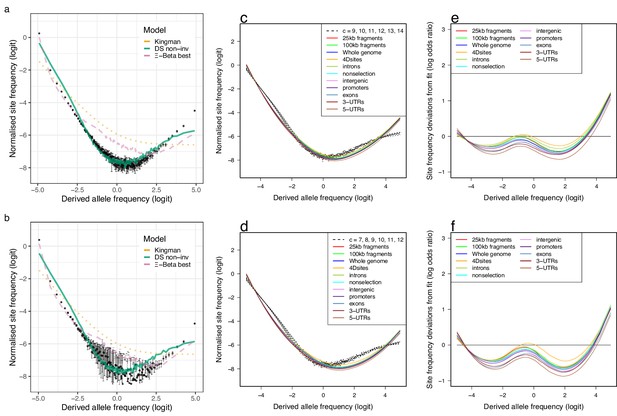
Fit to the selective sweepstakes model for GL2 estimated site-frequency spectra.

(**a, b**) Mean observed site-frequency spectra for the 19 non-inversion chromosomes combined estimated with GL2 likelihood for the South/south-east (sample size $n = 68$ ) and Þistilfjörður populations (sample size $n = 71$ ), respectively. Error bars of observed data are ±2 standard deviations of the bootstrap distribution with 100 bootstrap replicates. Expected site-frequency spectra are the Kingman coalescent (the no sweepstakes model), the best approximate maximum likelihood estimates (Eldon et al., 2015) of the $Ξ$ -Beta model (the random sweepstakes model), and the Durrett–Schweinsberg coalescent (DS) (the selective sweepstakes model) approximate Bayesian computation (ABC) estimated for the non-inversion chromosomes (non-inv). (**c, d**) The observed site-frequency spectra of different sized fragments and various functional classes compared to expectations of the Durrett–Schweinsberg coalescent (DS) ABC estimated for the non-inversion chromosomes for the South/south-east population and the Þistilfjörður population, respectively. The compound parameter $c$ ranges from 7 to 14. The different functional groups are fourfold degenerate sites (Dsites), intronic sites, non-selection sites (sites more than 500 kb away from peaks of selection scan, Appendix 6—figure 8), intergenic sites, promoters, exons, $3^{'}$ -UTR sites (3-UTRs), and $5^{'}$ -UTR (5-UTRs) sites in order of selective constraints. (e, f) Deviations from expectations of the Durrett–Schweinsberg model of recurrent selective sweeps of different sized fragments and functional groups for the South/south-east population and the Þistilfjörður population, respectively.

Appendix 6—figure 6

Download asset Open asset

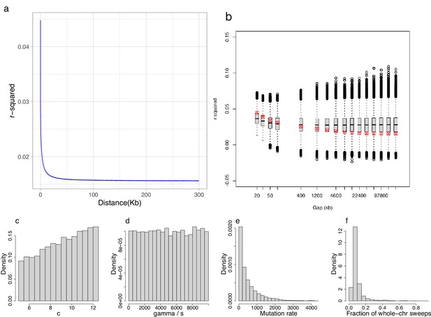
Decay of linkage disequilibrium with distance: observed and under an extension of the Durrett–Schweinsberg model.

(a) Observed linkage disequilibrium (LD), measured as $r^{2}$ , with distance in kb (kilobase). Non-inversion chromosomes from the South/south-east population as an example. LD decays rapidly to background values. (b) A subset of the distances from panel a (red × in circles) overlaid on the simulated empirical distribution of LD profiles (boxplot) obtained from the extension of the Durrett–Schweinsberg model described in Appendix 4. (**c–f** ) Posterior distributions of parameters from which panel b has been sampled. The $c$ parameter was constrained to lie between 5 and 12.5 to enforce consistency with the site-frequency spectrum (SFS)-based results in Figure 3 and Appendix 6—figure 7, while $γ / s$ and θ were constrained between 0 and 10,000 to avoid transient approximate Bayesian computation (ABC)-MCMC chains.

Appendix 6—figure 7

Download asset Open asset

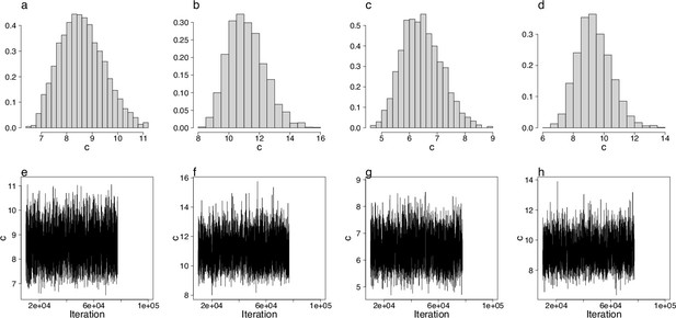
Approximate Bayesian computation (ABC) estimation of parameters of the Durrett–Schweinsberg coalescent (Durrett and Schweinsberg, 2005).

(**a–d**) ABC-posterior densities of the compound parameter $c \in Θ_{DS}$ using site-frequency spectra computed from likelihood GL1 (**a, c**) and GL2 (**b, d**) for the South/south-east and Þistilfjörður populations, respectively. (**e–h**) Corresponding trace plots demonstrating the good mixing of the ABC-MCMC.

Appendix 6—figure 8

Download asset Open asset

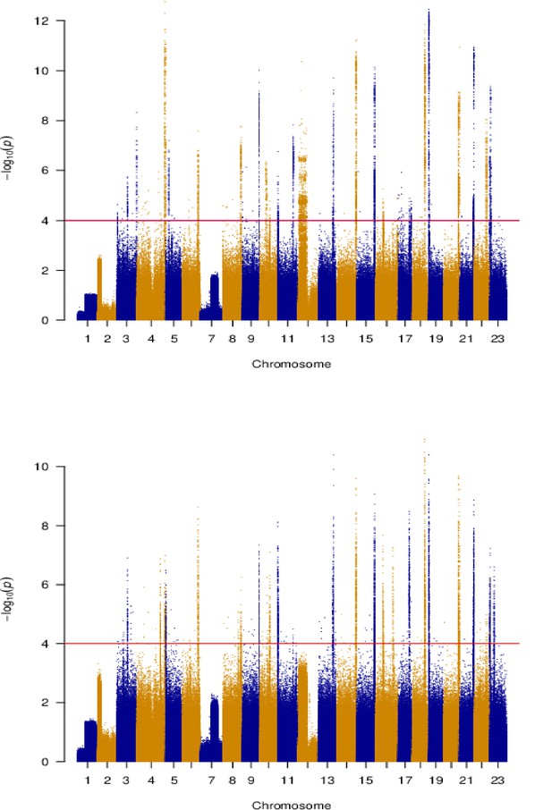
Principal components based genomic scan of selection for South/south-east (top) and Þistilfjörður (bottom) populations.

Regions of 500 kb on either side of peaks exceeding $- \log 10 p \geq 4$ were excluded to define regions of no selection for analysis in Figures 3 and 5.

Appendix 6—figure 9

Download asset Open asset

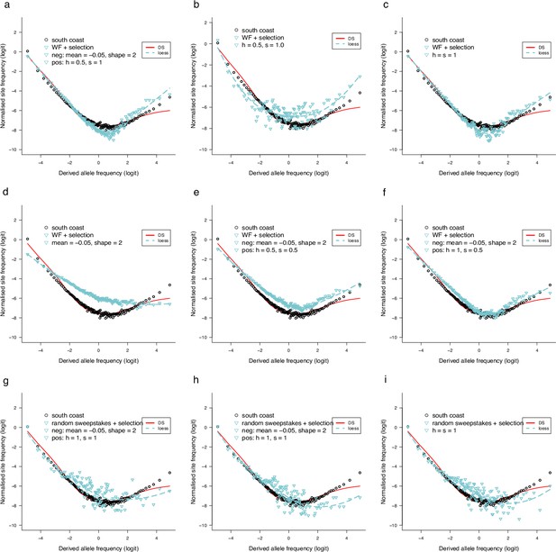
Observed site-frequency spectra compared to SLiM simulated site-frequency spectra under no-sweepstakes reproduction and random sweepstakes reproduction with selection.

Forward simulation using SLiM (Haller and Messer, 2019) of negative (background) selection and positive selection with variable dominance and with no-sweepstakes and random sweepstakes models of reproduction. (**a–f**) The Wright–Fisher no-sweepstakes model (population size $2 N = 10^{4}$ ) with selection. Negative mutations are modelled as a shifted gamma distribution with mean and shape as shown in each panel and with dominance $h = 1$ , and positive mutations with ﬁxed effects with dominance ( $h$ ) and selective advantage (selection coefficient $s$ ) as shown in each panel. In b and c, there is no negative selection but only positive mutations of ﬁxed effects with $h$ and $s$ as shown. In d, there are only negative mutations with same conﬁguration as in a. In e and f, both positive and negative mutations with conﬁgurations as shown. In **g–i**, random sweepstakes using a model in the domain of attraction of the $Ξ$ -Beta( $2 - α, α$ )-coalescent with population size $2 N = 2000$ , $α = 1.1$ (g) and $α = 1.25$ (**h, i**), with both negative and positive mutations in g and h with conﬁgurations as shown, and only positive mutations in i. In all graphs a loess regression curve is ﬁtted to the SLiM data points and compared to predictions of the Durrett–Schweinsberg (DS) coalescent with compound parameter $c = 6$ . The circles are site-frequency spectrum of chromosome 3 from the South/south-east coast population estimated with GL1 genotype likelihood. The scripts to generate the graphs are available at https://github.com/eldonb/selective-sweepstakes, (copy archived at swh:1:rev:3235fd1a87f2741b486cb9fe17a15ae85f605d26; Eldon, 2022b)

Appendix 6—figure 10

Download asset Open asset

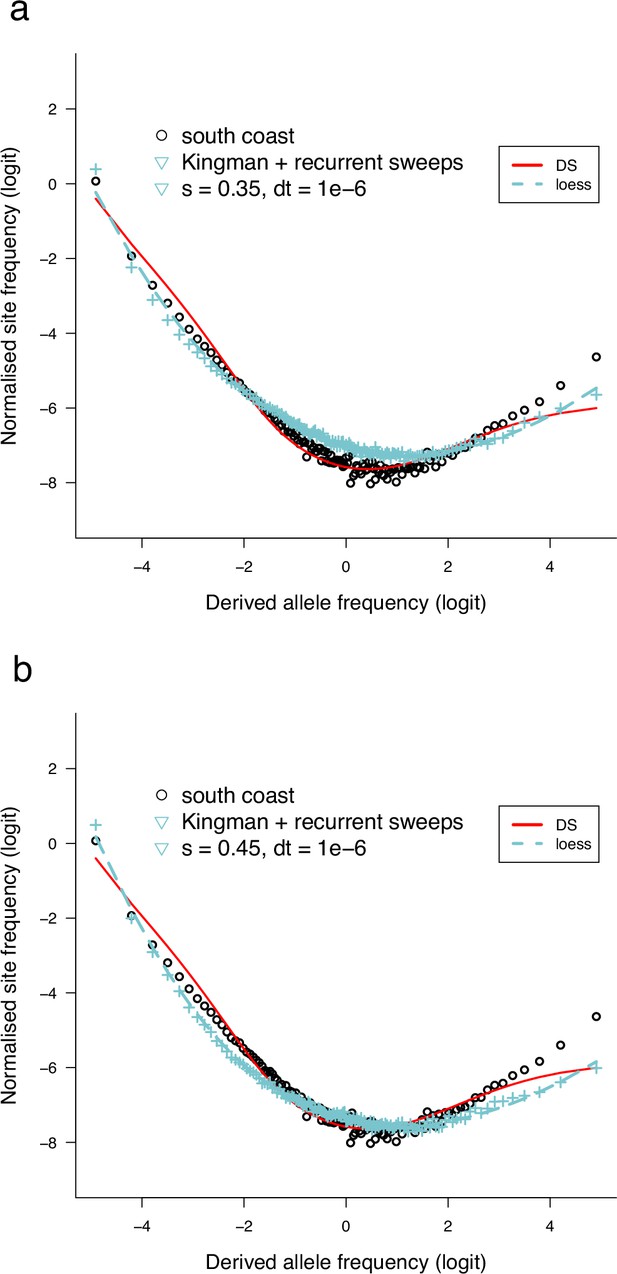
Observed site-frequency spectra compared to msprime simulated site-frequency spectra under Kingman coalescent with recurrent selective sweeps.

Backwards simulation using msprime (Baumdicker et al., 2021). (**a, b**) The standard Kingman coalescent model interrupted by randomly occurring hard sweeps. Each sweep with a selection coefficient $s$ (and time $d t$ between allele frequency updates) occurs at a random location on a chromosome of length 1 Mbp. msprime simulations of the Kingman coalescent and where hard sweeps occur at random times using a structured coalescent approach to model a sweep (Braverman et al., 1995), and msprime simulates a stochastic sweep trajectory according to a conditional diffusion model (Kim and Stephan, 2002; Coop and Griffiths, 2004). See the documentation of msprime for further details (tskit.dev/msprime/docs/stable/ancestry.html#sec-ancestry-models-selective-sweeps). The effective population size was $N_{e} = 10^{4}$ , mutation rate $μ = 10^{- 8}$ , and recombination rate. $γ = 10^{- 7}$ The circles represent the site-frequency spectrum of chromosome 3 (GL1) from the South/south-east coast population, and the red line is the normalized exact expected branch-length spectrum predicted by the Durrett–Schweinsberg coalescent with parameter $c = 6$ . The scripts to produce the graphs are available at https://github.com/eldonb.

Appendix 6—figure 11

Download asset Open asset

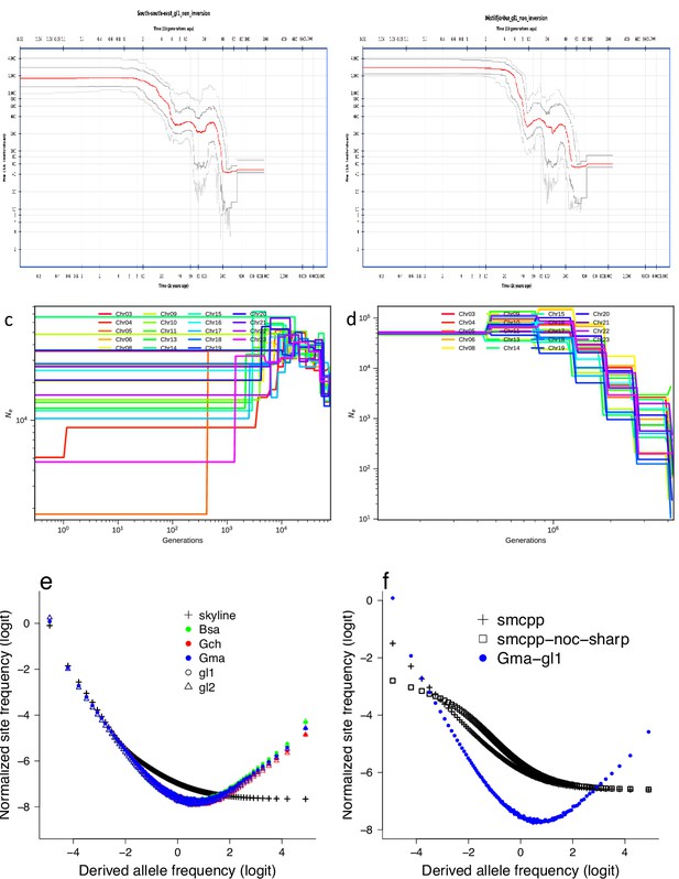
Estimated demographic history and frequency spectra from simulated demographic scenarios under the Kingman coalescent.

(top, left and right) Demographic history estimated with the stairway plot method (Liu and Fu, 2015; Liu and Fu, 2020) from the site-frequency spectra of the non-inversion chromosomes estimated with GL1 likelihoods of the South/south-east and Þistilfjörður population, respectively. Population expansion in the distant past and relative stability in more recent times. Demographic history estimated with smc++ (Terhorst et al., 2016) for the South/south-east population. smc++ run with default values (c) and treating runs of homozygosity as missing with the --missing-cutoff 10 flag (smcpp-noc-sharp) (d). Expected site-frequency spectra simulated using msprime (Kelleher et al., 2016; Baumdicker et al., 2021) based on the demographic scenarios of the stairway plot (e) and the smc++ (f) for the South/south-east population. The observed site-frequency spectra of the non-inversion chromosomes of the South/south-east population estimated using the GL1 and GL2 likelihoods and polarized using different outgroups (Bsa, Gch, and Gma) (e). For the smc ++ comparison the observed data are the average of the non-inversion chromosomes of the South/south-east population estimated using the GL1 genotype likelihood and polarized with Gma as outgroup (f).

Appendix 6—figure 12

Download asset Open asset

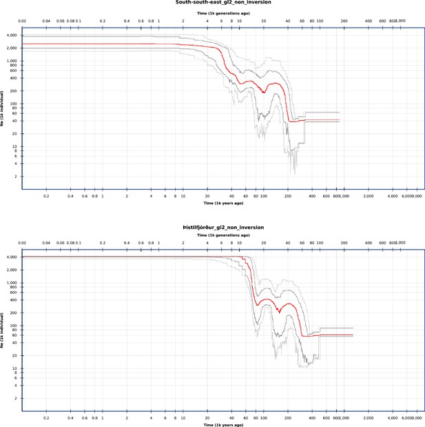
Stairway plots of demographic history of the populations of GL2 likelihood data.

Demographic history estimated from the site-frequency spectra of the non-inversion chromosomes based on GL2 likelihoods for the South/south-east (top) and the Þistilfjörður (bottom) populations, respectively, with the stairway plot method (Liu and Fu, 2015; Liu and Fu, 2020).

Appendix 6—figure 13

Download asset Open asset

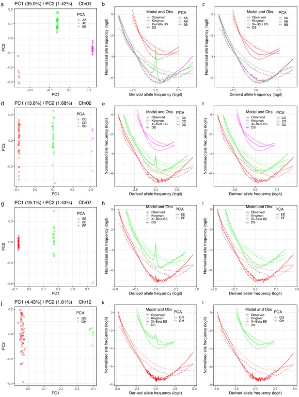
Groups from principal component analysis (PCA), conjectured as cryptic population structure, and observed site-frequency spectra compared to coalescent expectations.

(**a, d, g, j**) Groups revealed by PCA of variation at inversion chromosomes Chr01, Chr02, Chr07, and Chr12, respectively, conjectured to represent cryptic population structure that should extend to the whole genome. (**b, e, h, k**) The site-frequency spectra estimated for the groups of the respective inversion chromosome using variation at each inversion chromosome. (**c, f, i, l**) The site-frequency spectra estimated for the groups of the respective inversion chromosome using variation at the 19 non-inversion chromosomes. Observed site-frequency spectra compared to expectations based on the Kingman, 1982 (no-sweepstakes), the $Ξ$ -Beta( $2 - α, α$ ) coalescent (Schweinsberg, 2000) (random sweepstakes) with $α = 1$ (the Bolthausen–Sznitman coalescent, BS), and the Durrett-Schweinsberg coalescent (Durrett and Schweinsberg, 2005) of recurrent selective sweeps (DS) approximate Bayesian computation (ABC) estimated for the PCA groups of each chromosome. Data from the South/south-east population. Non-inversion chromosomes show no peaks at intermediate frequencies as expected under the conjecture. The conjecture of cryptic population structure is rejected.

Appendix 6—figure 14

Download asset Open asset

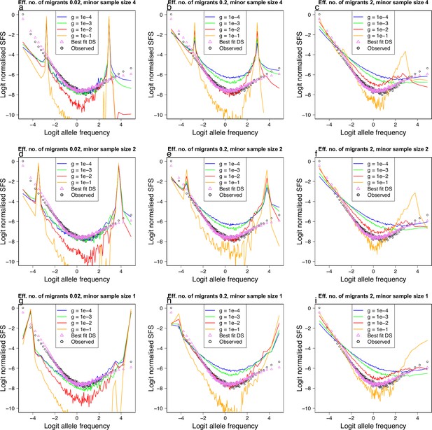
Population structure, isolation with migration, and population growth under the Kingman coalescent.

(**a–i**) Simulations using msprime (Kelleher et al., 2016; Baumdicker et al., 2021) of the effects of a mixed sample of two divergent populations evolving under the Kingman coalescent (no sweepstakes model) with population growth on the expected site-frequency spectrum. A two island model with migration rate $m$ and per-generation population growth rate $g$ . The effective number of migrants ( $N_{e} m$ ) increases from 0.02 to 2, and hence the degree of isolation decreases, going from left to right. The sample size of the minor populations (the population from which fewer individuals are sampled) decreases from top to bottom (minor sample size 4…1). The effects of population growth $g$ displayed with different colours. Simulated model expectations (solid lines) compared to observed data (circles) of chromosome 4 estimated with GL1 and Gma as outgroup from the South/south-east population for comparison. Also included are the expectation of the Durrett–Schweinsberg coalescent (Durrett and Schweinsberg, 2005) (selective sweepstakes model, best-fit DS: triangle) to observations. (i) Only a minor sample size of one combined with the highest rate of migration and particular growth rates gives closest resemblance to observations.

Appendix 6—figure 15

Download asset Open asset

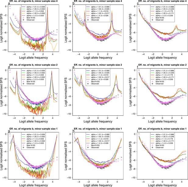
Population structure, isolation with migration, and population growth under the Xi-Beta coalescent.

(**a-i**) Simulations using msprime (Kelleher et al., 2016; Baumdicker et al., 2021) of the effects of a mixed sample of two divergent populations evolving under the $Ξ$ -Beta( $2 - α, α$ ) coalescent (the random sweepstakes model) on the expected site-frequency spectrum. A two island model with migration and different values of the $α$ parameter (displayed with different colours). The effective number of migrants $b$ (comparable to $N_{e} m$ in Appendix 6—figure 14) increases, and hence the degree of isolation decreases, going from left to right. The sample size of the minor populations decreases from top to bottom (4–1). Simulated model expectations (solid lines) compared to observed data (circles) of chromosome 4 estimated with GL1 and Gma as outgroup from the South/south-east population for comparison. Also included are the expectation of the Durrett–Schweinsberg coalescent (Durrett and Schweinsberg, 2005) (selective sweepstakes model, best-fit DS: triangle) to observations. (i) Only a minor sample size of one combined with the highest rate of migration and particular values of $α$ gives closest resemblance to observations.

Appendix 6—figure 16

Download asset Open asset

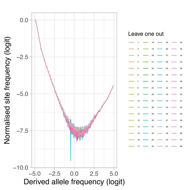
Estimated site-frequency spectra with a leave-one-out approach.

Estimated site-frequency spectra for chromosome 4 of 67 individuals leaving out each individual in turn from the 68 individuals of the South/south-east population. Circles are site-frequency spectrum of the original sample of 68 individuals. Based on the simulations results in Appendix 6—figure 14 and Appendix 6—figure 15 that a minor sample size of one can resemble model expectations, one of the leave-one-out samples should be divergent if the sample of 68 individuals is composed of 67 individuals from one population and a single individual from a divergent population. None of the leave-one-out samples is off so this conjecture is rejected.

Appendix 6—figure 17

Download asset Open asset

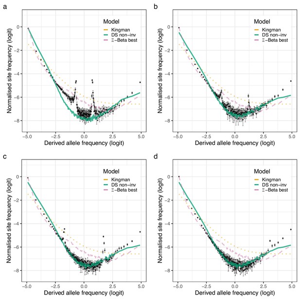
Observed site-frequency spectra at inversion chromosomes and coalescent expectations for the South/south-east population.

(**a–d**) Observed site-frequency spectra estimated with GL1 for the four inversion chromosomes, chromosome 1 (Chr01), chromosome 2 (Chr02), chromosome 7 (Chr07), and chromosome 12 (Chr12), respectively in the South/south-east population (sample size $n = 68$ ). Error bars are ±2 standard deviations of the bootstrap distribution with 100 bootstrap replicates. Expected site-frequency spectra are the Kingman coalescent (the no sweepstakes model), the Durrett–Schweinsberg (DS) coalescent (selective sweepstakes model) approximate Bayesian computation (ABC) estimated for the non-inversion chromosomes (DS non-inv), and the best approximate maximum likelihood estimates (Eldon et al., 2015) of the $Ξ$ -Beta model (the random sweepstakes model). The best estimated $\hat{α}$ values were ${\hat{α}}_{Ξ} = 1.16$ , ${\hat{α}}_{Ξ} = 1.16$ , ${\hat{α}}_{Ξ} = 1.16$ , and ${\hat{α}}_{Ξ} = 1.12$ , for chromosomes 1, 2, 7, and 12, respectively.

Appendix 6—figure 18

Download asset Open asset

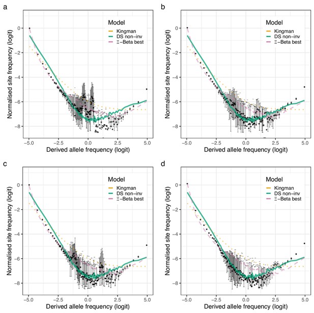
Observed site-frequency spectra at inversion chromosomes and coalescent expectations for the Þistilfjörður population.

(**a–d**) Observed site-frequency spectra estimated with GL1 for the four inversion chromosomes, chromosome 1 (Chr01), chromosome 2 (Chr02), chromosome 7 (Chr07), and chromosome 12 (Chr12), respectively for the Þistilfjðrður population (sample size $n = 71$ ). Error bars are ±2 standard deviations of the bootstrap distribution with 100 bootstrap replicates. Expected site-frequency spectra are the Kingman coalescent (the no sweepstakes model), the Durrett–Schweinsberg (DS) coalescent (selective sweepstakes model) approximate Bayesian computation (ABC) estimated for the non-inversion chromosomes (non-inv), and the best approximate maximum likelihood estimates (Eldon et al., 2015) of the $Ξ$ -Beta model (the random sweepstakes model). The best estimated $\hat{α}$ values are ${\hat{α}}_{Ξ} = 1.18$ , ${\hat{α}}_{Ξ} = 1.16$ , ${\hat{α}}_{Ξ} = 1.17$ , and ${\hat{α}}_{Ξ} = 1.08$ , for chromosomes 1, 2, 7, and 12, respectively.

Appendix 6—figure 19

Download asset Open asset

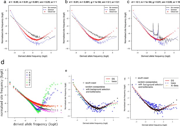
Observed site-frequency spectra compared to SLiM forward simulated site-frequency spectra based on demographic scenarios with and without selective sweeps and with background selection and recurrent bottlenecks.

Forward simulation using SLiM (Haller and Messer, 2019). (**a–c**) Each scenario has two islands of initial population size 300. Both islands undergo exponential growth at per-generation rate $g$ until a total size of 1000. The per-generation migration probability is $m$ . The SLiM simulation is run until the whole population has a MRCA, at which point 136 haploid genomes (as the sample from the South/south-east population) are drawn from the population. Each scenario is simulated 1000 times to estimate the mean normalized site-frequency spectrum. The genome length is set to 100 kb, and the recombination and mutation rates are 10⁻⁸ per site per generation. The ‘No sweeps’ scenario undergoes deleterious mutations with fitness effects described by a gamma distribution with mean $d$ and shape parameter 0.2. The ‘Sweeps’ scenario has the same deleterious mutations, and also beneficial mutations with a fixed fitness effect of $s m$ . The relative rate of these positive mutations to the deleterious ones is $s r$ . The observed site-frequency spectrum is the mean of the 100 kb fragments across all non-inversion chromosomes. Only sweeps scenarios show U-shaped site-frequency spectra. (d) Results of simulations of background selection. In all cases a population of size $N = 10^{5}$ evolves according to the Wright–Fisher model assuming a chromosome segment of size 10⁵ bp with recombination rate 10⁻⁷ per site per generation that collects neutral or negative mutations with frequency $μ = 10^{- 7}$ per site per generation. Negative mutations were modelled as Gamma-distributed with a negative sign, with mean −0.1 (**a, b, d**) or −0.05 (**c, e, f**) all with shape parameter 0.2. The relative frequency of negative versus neutral mutations was 1:1 for (**a, b, d**) and 1:9 for (**c, e, f**). The points represent the logits of the normalized site-frequency spectrum of a random sample of 136 chromosomes (corresponding to the sample size of the South/south-east population) averaged over 100 (**a, b, d, e**) and 10 (**d, f**) replicates and taken after 10⁵ generations (**b, e**), 2 × 10⁵ generations (**a, c**), and 10⁶ generations (**d, f**). U-shaped site-frequency spectra only found for short runs (**b, e**). (e, f) Simulations were produced by the C++ simulation code forward available at https://github.com/eldonb/forward; Eldon, 2022a for individual-based forward-in-time simulations with random sweepstakes, randomly occurring bottlenecks, and selection. Haploid model in e and diploid model in f.

Appendix 6—figure 20

Download asset Open asset

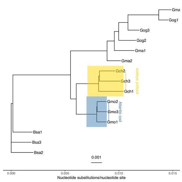
Neighbour joining tree of gadid taxa.

Based on $p$ -distance (nucleotide substitutions per nucleotide site) of whole genome among the gadid taxa Atlantic cod (*Gadus morhua*, Gmo), walleye pollock (*G. chalcogramma*, Gch), Pacific cod (*G. macrocephalus*, Gma), Greenland cod (*G. ogac*, Gog), and Arctic cod (*Boreogadus saida*, Bsa). Under the assumption that the focal taxa, Atlantic cod and walleye pollock, diverged 3.5 × 10⁶ years ago (Vermeij, 1991; Vermeij and Roopnarine, 2008; Coulson et al., 2006; Carr and Marshall, 2008), the distance between these taxa is used for mutation rate estimation in Appendix 7—table 4.

Appendix 6—figure 21

Download asset Open asset

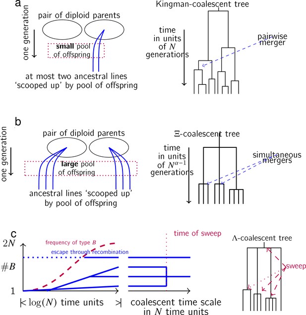
Schematic illustration of the three coalescent models, Kingman (no sweepstakes), Xi-Beta (random sweepstakes), and DS (selective sweepstakes).

(a) In each generation, any given pair of diploid parents in a low-fecundity population produces only a small number of offspring, a no-sweepstakes scenario. At most two ancestral lineages (shown as blue lines) of a sample can, therefore, be involved in a given family with non-negligible probability in a large population, leading to at most two ancestral lineages merging each time when the ancestral tree is viewed on a coalescent timescale of $N$ generations per coalescent time unit. (b) In a highly fecund population reproducing according to random sweepstakes reproduction, a given pair of diploid parents may produce a huge number of offspring, scooping up a number of ancestral lineages of a sample (shown as blue lines) in an instance of random sweepstakes. The resulting gene genealogy may include multiple and simultaneous multiple mergers of ancestral lineages of a sample. (c) An example of the effects of selective sweepstakes through repeated selective sweeps on the genealogy of a neutral site. Shown is a hypothetical history of ancestral lineages of a sample (blue lines) at the neutral site during a sweep of the beneficial allelic type $B$ at a site different from the neutral site. At the start of a sweep a single chromosome not ancestral to the sample experiences a mutation to type $B$ . During the sweep one of the ancestral chromosomes has several descendants while another (shown in dotted blue lines) manages to ‘escape’ a sweep by recombining onto a ‘b’ background. At the end of the sweep all chromosomes have a ‘B’ background, however, not all of the ancestral lineages will trace back to the initial $B$ chromosome. Since we are only interested in the genealogy at the neutral site only the ancestral relations of the neutral site are shown (blue lines). Viewed on a coalescent timescale of $N$ time units per one coalescent time unit, the sweep happens instantaneously, and thus appears as an instantaneous merger of three lineages in the genealogy of the neutral site.

Appendix 6—figure 22

Download asset Open asset

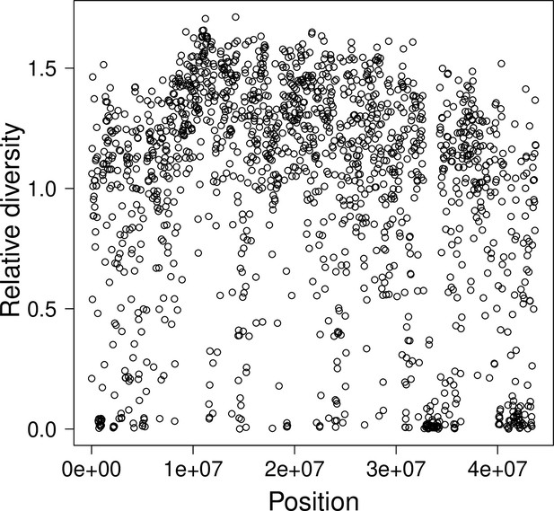
Relative diversity and the compound parameter $c$ along chromosome 4.

The compound parameter $c = δ s^{2} / γ$ of the Durrett–Schweinsberg model measures the rate of selective sweeps (δ) times the squared selection coefficient ( $s^{2}$ ) of the beneficial mutation over the recombination rate (γ) between the selected site and the neutral site of interest. The compound parameter $c$ can be considered to be essentialy the density of selection per map unit along a chromosome (Aeschbacher et al., 2017). The number of single nucleotide polymorphisms (SNPs) in a 25 k fragment is proportional to branch length, which again is proportional to the compound parameter $c$ . The relative diversity is the number of SNPs normalized by the mean number of SNPs on chromosome fragment location is indicative of the density of selection along a chromosome.

Tables

Appendix 7—table 1

Diversity and neutrality test statistics for the South/south-east population.

Watterson’s estimator of the population scaled mutation rate per nucleotide site $θ_{W}$ , the pairwise nucleotide diversity per nucleotide site $θ_{π}$ , Tajima’s $D_{T}$ , Fu and Li’s $D_{F}$ , and number of nucleotide sites based on GL1 and GL2 likelihoods (sample size $n = 68$ ).

	GL1 likelihood					GL2 likelihood
	$θ_{W}$	$θ_{π}$	$D_{T}$	$D_{F}$	nSites	$θ_{W}$	$θ_{π}$	$D_{T}$	$D_{F}$	nSites
Chr01	0.0046	0.0024	−1.64	−5.77	18332422	0.0056	0.0025	−1.84	−6.71	18332093
Chr02	0.0050	0.0020	−1.98	−6.00	15828347	0.0060	0.0022	−2.11	−6.84	15828079
Chr03	0.0053	0.0020	−2.09	−6.22	20202769	0.0063	0.0021	−2.21	−6.98	20202435
Chr04	0.0054	0.0020	−2.08	−6.03	22584280	0.0065	0.0022	−2.19	−6.79	22583924
Chr05	0.0053	0.0020	−2.10	−6.22	15542562	0.0064	0.0021	−2.22	−6.99	15542313
Chr06	0.0052	0.0019	−2.11	−6.33	17720989	0.0062	0.0021	−2.22	−7.09	17720709
Chr07	0.0056	0.0022	−2.01	−5.88	21080002	0.0066	0.0024	−2.13	−6.64	21079620
Chr08	0.0054	0.0020	−2.09	−6.09	18353883	0.0065	0.0022	−2.21	−6.85	18353624
Chr09	0.0053	0.0019	−2.13	−6.42	18195728	0.0063	0.0021	−2.25	−7.16	18195437
Chr10	0.0051	0.0019	−2.09	−6.27	17450729	0.0061	0.0020	−2.21	−7.06	17450432
Chr11	0.0050	0.0018	−2.14	−6.54	20138893	0.0059	0.0019	−2.26	−7.32	20138619
Chr12	0.0043	0.0016	−2.14	−6.32	19448827	0.0053	0.0017	−2.26	−7.18	19448580
Chr13	0.0049	0.0018	−2.14	−6.38	18651575	0.0059	0.0019	−2.26	−7.18	18651311
Chr14	0.0053	0.0019	−2.14	−6.34	20704894	0.0063	0.0020	−2.25	−7.09	20704623
Chr15	0.0054	0.0019	−2.17	−6.41	18100213	0.0064	0.0020	−2.27	−7.15	18099944
Chr16	0.0051	0.0019	−2.09	−6.13	22233178	0.0061	0.0021	−2.21	−6.93	22232862
Chr17	0.0053	0.0020	−2.06	−5.99	11813809	0.0063	0.0022	−2.18	−6.78	11813609
Chr18	0.0053	0.0019	−2.11	−6.23	15931558	0.0063	0.0021	−2.23	−7.01	15931312
Chr19	0.0055	0.0020	−2.10	−6.23	13858302	0.0065	0.0022	−2.21	−6.98	13858066
Chr20	0.0050	0.0018	−2.15	−6.56	16371168	0.0059	0.0019	−2.27	−7.33	16370967
Chr21	0.0052	0.0019	−2.10	−6.29	14440220	0.0062	0.0021	−2.22	−7.07	14440024
Chr22	0.0054	0.0020	−2.08	−6.12	13838440	0.0065	0.0022	−2.19	−6.89	13838214
Chr23	0.0052	0.0020	−2.08	−6.27	14698719	0.0062	0.0021	−2.20	−7.05	14698473
All	0.0052	0.0019	−2.08	−6.22	17631370	0.0062	0.0021	−2.20	−7.00	17631099

Appendix 7—table 2

Diversity and neutrality test statistics for the Þistilfjörður population.

$θ_{W}$ Watterson’s estimator of the population scaled mutation rate per nucleotide site, $θ_{π}$ the pairwise nucleotide diversity per nucleotide site, Tajima’s $D_{T}$ , Fu and Li’s $D_{F}$ , and number of nucleotide sites based on GL1 and GL2 likelihoods (sample size $n = 71$ ).

	GL1 likelihood					GL2 likelihood
	$θ_{W}$	$θ_{π}$	$D_{T}$	$D_{F}$	nSites	$θ_{W}$	$θ_{π}$	$D_{T}$	$D_{F}$	nSites
Chr01	0.0068	0.0037	−1.51	−5.99	16159362	0.0090	0.0040	−1.84	−7.55	16159148
Chr02	0.0069	0.0030	−1.86	−6.18	14306627	0.0092	0.0034	−2.10	−7.65	14306351
Chr03	0.0073	0.0029	−1.99	−6.38	18283815	0.0096	0.0033	−2.19	−7.76	18283555
Chr04	0.0074	0.0030	−1.97	−6.14	20435443	0.0097	0.0034	−2.17	−7.52	20435122
Chr05	0.0073	0.0029	−2.00	−6.36	13933982	0.0096	0.0032	−2.20	−7.74	13933752
Chr06	0.0072	0.0028	−2.00	−6.46	16048768	0.0094	0.0032	−2.21	−7.84	16048531
Chr07	0.0076	0.0034	−1.83	−6.06	19008270	0.0099	0.0038	−2.05	−7.46	19007926
Chr08	0.0074	0.0030	−1.98	−6.20	16559106	0.0097	0.0033	−2.18	−7.59	16558861
Chr09	0.0073	0.0028	−2.03	−6.59	16381498	0.0096	0.0032	−2.23	−7.93	16381249
Chr10	0.0070	0.0028	−1.98	−6.42	15789838	0.0093	0.0032	−2.19	−7.83	15789584
Chr11	0.0069	0.0026	−2.04	−6.73	18211081	0.0091	0.0029	−2.24	−8.12	18210846
Chr12	0.0061	0.0024	−2.03	−6.52	17597347	0.0082	0.0027	−2.24	−8.07	17597135
Chr13	0.0068	0.0026	−2.04	−6.58	16846892	0.0090	0.0029	−2.24	−8.01	16846697
Chr14	0.0073	0.0028	−2.04	−6.52	18699877	0.0095	0.0031	−2.23	−7.89	18699625
Chr15	0.0074	0.0028	−2.06	−6.54	16349327	0.0097	0.0031	−2.25	−7.86	16349118
Chr16	0.0070	0.0028	−1.98	−6.27	20259494	0.0092	0.0032	−2.19	−7.71	20259231
Chr17	0.0072	0.0030	−1.93	−6.09	10667396	0.0095	0.0033	−2.15	−7.52	10667225
Chr18	0.0072	0.0029	−2.00	−6.39	14305479	0.0095	0.0032	−2.21	−7.79	14305261
Chr19	0.0075	0.0030	−1.98	−6.33	12465223	0.0098	0.0034	−2.18	−7.68	12465024
Chr20	0.0069	0.0026	−2.06	−6.73	14829191	0.0091	0.0029	−2.25	−8.11	14829009
Chr21	0.0071	0.0029	−1.99	−6.43	13014009	0.0094	0.0032	−2.20	−7.83	13013813
Chr22	0.0074	0.0030	−1.97	−6.30	12407034	0.0097	0.0034	−2.17	−7.70	12406815
Chr23	0.0072	0.0029	−1.97	−6.40	13273011	0.0094	0.0032	−2.18	−7.81	13272801
All	0.0071	0.0029	−1.97	−6.37	15905742	0.0094	0.0032	−2.18	−7.78	15905508

Appendix 7—table 3

Demographic statistics, correction factor, $C$ , and generation length, $G$ , of female component of Atlantic cod in Iceland.

Age-specific survival rate, l_i, was based, respectively, on the average and the 1948–1952 and the 1963–1967 instantaneous mortality estimated from tagging experiments of Icelandic cod (Jónsson, 1996). Age-specific fecundity based on the average age-specific weight in catch (Anonymous, 2001) and fecundity by weight relationships (Marteinsdottir and Begg, 2002) and similar relationships for Newfoundland cod for comparison (May, 1967). The $C$ and $G$ are, respectively, the correction factor for the effects of overlapping generations and generation time based on demographic estimation (Jorde and Ryman, 1995; Jorde and Ryman, 1996; Laikre et al., 1998) and iteration of Equations 5–9 in Jorde and Ryman, 1996. Table is truncated at Age class 15 for lack of population data on older age classes.

Age	Age		’48–’52	’63–’67	GM	May
Age	class	${\bar{l}}_{i}$	l_i	l_i	$b_{i} \times 10^{6}$	$b_{i} \times 10^{6}$
0	1	1.0000	1.0000	1.0000	0.00	0
1	2	0.3396	0.4966	0.2369	0.00	0
2	3	0.1153	0.2466	0.0561	0.00	0
3	4	0.0392	0.1225	0.0133	0.38	0.52
4	5	0.0133	0.0608	0.0032	0.62	0.78
5	6	0.0045	0.0302	0.0007	1.01	1.15
6	7	0.0015	0.0150	0.0002	1.59	1.67
7	8	0.0005	0.0074	0.0000	2.37	2.31
8	9	0.0002	0.0037	0.0000	3.28	3.03
9	10	0.0001	0.0018	0.0000	4.24	3.73
10	11	0.0000	0.0009	0.0000	5.30	4.48
11	12	0.0000	0.0005	0.0000	6.41	5.24
12	13	0.0000	0.0002	0.0000	7.68	6.07
13	14	0.0000	0.0001	0.0000	8.79	6.78
14	15	0.0000	0.0001	0.0000	10.42	7.79
$C$		10.5	7.9	17.6		20.0
$G$		5.1	6.3	4.6		4.6
$C / G$		2.1	1.3	3.8		3.8

Appendix 7—table 4

Genetic divergence between the Atlantic cod and walleye pollock sister taxa and rate of evolution.

The $p$ -distance, the proportion of sites per nucleotide site that differ between the sister taxa Atlantic cod and walleye pollock (Appendix 6—figure 20) estimated with ngsDist (Vieira et al., 2015) setting the total number of sites (--tot_sites) equal to the number of sites that pass quality filtering in the estimation of site-frequency spectra (Appendix 7—table 7). The mutation rate μ which is the $p$ -distance per nucleotide site per year are calculated under the assumption that these taxa diverged $3.5 \times 10^{6}$ years ago (Vermeij, 1991; Vermeij and Roopnarine, 2008; Coulson et al., 2006; Carr and Marshall, 2008). The number of substitutions per year, based on the number of sites in each chromosome (chromosomal length, last column), and its inverse, the number of years per substitution, are the rates for either lineage. Also given are the average over the chromosomes, and the whole-genome numbers. Based on the overall $p$ -distances between the Atlantic cod sample from the South/south-east population (sample size $n = 68$ ) and a sample of 36 walleye pollock from a single locality in the Gulf of Alaska.

Chromosome	$p$ per site	$μ = p$ per site per year	Number of substitutions per year	Number of years per substitution	Number of sites
Chr01	0.00504	$7.21 \times 10^{- 10}$	0.022	45	30875876
Chr02	0.00500	$7.14 \times 10^{- 10}$	0.021	49	28732775
Chr03	0.00492	$7.03 \times 10^{- 10}$	0.022	46	30954429
Chr04	0.00490	$7.00 \times 10^{- 10}$	0.031	33	43798135
Chr05	0.00512	$7.31 \times 10^{- 10}$	0.018	54	25300426
Chr06	0.00508	$7.25 \times 10^{- 10}$	0.020	50	27762770
Chr07	0.00511	$7.29 \times 10^{- 10}$	0.025	40	34137969
Chr08	0.00497	$7.11 \times 10^{- 10}$	0.021	47	29710654
Chr09	0.00518	$7.40 \times 10^{- 10}$	0.020	51	26487948
Chr10	0.00513	$7.33 \times 10^{- 10}$	0.020	50	27234273
Chr11	0.00505	$7.22 \times 10^{- 10}$	0.022	45	30713045
Chr12	0.00495	$7.08 \times 10^{- 10}$	0.022	46	30948897
Chr13	0.00523	$7.47 \times 10^{- 10}$	0.022	46	28829685
Chr14	0.00508	$7.26 \times 10^{- 10}$	0.021	47	29586942
Chr15	0.00499	$7.13 \times 10^{- 10}$	0.020	49	28657694
Chr16	0.00498	$7.12 \times 10^{- 10}$	0.025	40	34794352
Chr17	0.00502	$7.16 \times 10^{- 10}$	0.016	64	21723002
Chr18	0.00513	$7.33 \times 10^{- 10}$	0.018	55	24902675
Chr19	0.00529	$7.56 \times 10^{- 10}$	0.017	60	22015597
Chr20	0.00506	$7.23 \times 10^{- 10}$	0.018	56	24843429
Chr21	0.00521	$7.45 \times 10^{- 10}$	0.017	60	22358821
Chr22	0.00516	$7.37 \times 10^{- 10}$	0.018	57	23744039
Chr23	0.00529	$7.56 \times 10^{- 10}$	0.019	52	25242006
Average	0.00508	$7.26 \times 10^{- 10}$	0.021	49	28406758
Genome	0.00507	$7.25 \times 10^{- 10}$	0.474	2	653355439

Appendix 7—table 5

A list of key terms and a brief description.

Term	Description
High fecundity	The ability of organisms (e.g. broadcast spawners) to produce huge numbers of offspring, or on the order of the population size
Sweepstakes reproduction	High variance and high skew in the distribution of number of offspring, where most of the time individuals produce small (relative to the population size) number of offspring, but occasionally a few individuals contribute the bulk of the offspring forming a new generation of reproducing individuals
Random sweepstakes	A chance matching of reproduction in a highly fecund population with favorable environmental conditions; random sweepstakes is one example of a mechanism turning high fecundity into sweepstakes reproduction
Selective sweepstakes	A mechanism turning high fecundity into sweepstakes reproduction, in which juveniles pass through selective filters during their development, resulting in highly skewed offspring distribution
Moran model	A population model of genetic reproduction, in which a single random individual produces one offspring replacing another individual that perishes to keep the population size constant
Genealogy	The ancestral relations of a sample of gene copies (see Appendix 6—figure 21)
Coalescent	A probabilistic model of the random ancestral relations of a hypothetical sample of gene copies
Multiple-merger coalescent	A coalescent process in which a random number of ancestral lineages merges each time (see Appendix 6—figure 21)
$Ξ$ -Beta $(2 - α, α)$ -coalescent	A multiple-merger coalescent derived from a model of random sweepstakes
Durrett–Schweinsberg model	A model of recurrent selective sweeps of a new beneficial mutation each time approximating selective sweepstakes
Durrett–Schweinsberg coalescent	A coalescent model for the genealogy at a single site linked to a site experiencing beneficial mutation; during a sweep some lineages of the neutral site may escape a sweep through recombination (see Appendix 6—figure 21)

Appendix 7—table 6

Approximate Bayesian computation (ABC) priors of parameter for various analysis.

Parameter	ABC prior
$α$ for the Beta ( $2 - α, α$ )-coalescent	Uniform between 1.01 and 1.99
$β$ , the growth rate for the Beta ( $2 - α, α$ )-coalescent with population growth	Improper, uniform prior on the whole positive half-line
$c$ for the single-locus DS model	Improper, uniform prior on the whole positive half-line
$c$ for the DS model with recombination	Uniform between 10 and 25 (to force consistency with the posterior in the single-locus analysis)
$γ / s$ , the ratio of the recombination rate and the selection coefficient, in the DS model with recombination	Uniform between 0 and 10,000
θ, the mutation rate in the DS model with recombination	Uniform between 0 and 10,000
Fraction of whole-chromosome sweeps in the DS model with recombination	Uniform between 0 and 1

Appendix 7—table 7

Genetic divergence between the Atlantic cod and walleye pollock sister taxa and rate of evolution from GL1 estimated site-frequency spectra.

The site-frequency spectrum of the South/south-east population of Atlantic cod estimated with ANGSD and genotype likelihood GL1 (Korneliussen et al., 2014), using walleye pollock (Gch) as outgroup to polarise the spectrum, gives all sites that pass quality filtering $L$ , the number of invariant sites $I$ , the number of segregating sites $S$ , and the number of fixed sites $F$ between the focal population and the outgroup taxon. The number of substitutions per year and the number of years per substitution are calculated from fixed sites under the assumption that these taxa diverged $3.5 \times 10^{6}$ years ago (Vermeij, 1991; Vermeij and Roopnarine, 2008; Coulson et al., 2006; Carr and Marshall, 2008). The average over the chromosomes and the whole-genome numbers are also given. Compare to Appendix 7—table 4 and Appendix 7—table 8.

Chromosome	All sites, $L$	Invariant sites, $I$	Segregating sites, $S$	Fixed sites, $F$	Substitutions per year	Years per substitution
Chr01	18350418	17736728	468247	145443	0.042	24
Chr02	15850624	15269222	437440	143962	0.041	24
Chr03	20231166	19467361	592044	171761	0.049	20
Chr04	22623179	21742567	673837	206775	0.059	17
Chr05	15557754	14963290	457852	136612	0.039	26
Chr06	17738562	17090577	506727	141258	0.040	25
Chr07	21107906	20282169	645738	180000	0.051	19
Chr08	18381649	17681336	549023	151290	0.043	23
Chr09	18212083	17528065	533448	150571	0.043	23
Chr10	17472145	16829837	491408	150899	0.043	23
Chr11	20157683	19439102	550466	168115	0.048	21
Chr12	19475709	18838352	465219	172138	0.049	20
Chr13	18669907	18002288	504278	163341	0.047	21
Chr14	20723905	19946397	605101	172407	0.049	20
Chr15	18123369	17435024	538832	149513	0.043	23
Chr16	22268819	21460587	624520	183712	0.052	19
Chr17	11831346	11376461	344921	109964	0.031	32
Chr18	15955850	15348766	461840	145244	0.041	24
Chr19	13869827	13314508	421341	133978	0.038	26
Chr20	16390870	15807585	448550	134735	0.038	26
Chr21	14455156	13911966	414247	128943	0.037	27
Chr22	13854159	13314972	413965	125222	0.036	28
Chr23	14714440	14154540	424496	135403	0.039	26
Mean	17652892	16997465	503197	152230	0.043	23
Genome	406016526	390941701	11573540	3501286	1.000	1

Appendix 7—table 8

Genetic divergence between the Atlantic cod and walleye pollock sister taxa and rate of evolution from GL2 estimated site-frequency spectra.

The site-frequency spectrum of the South/south-east population of Atlantic cod estimated with ANGSD and genotype likelihood GL2 (Korneliussen et al., 2014), using walleye pollock (Gch) as outgroup to polarize the spectrum, gives all sites that pass quality filtering $L$ , the number of invariant sites $I$ , the number of segregating sites $S$ , and the number of fixed sites $F$ between the focal population and the outgroup taxon. The number of substitutions per year and the number of years per substitution are calculated from fixed sites under the assumption that these taxa diverged $3.5 \times 10^{6}$ years ago (Vermeij, 1991; Vermeij and Roopnarine, 2008; Coulson et al., 2006; Carr and Marshall, 2008). The average over the chromosomes and the whole-genome numbers are also given. Compare to Appendix 7—table 4 and Appendix 7—table 7.

Chromosome	All sites, $L$	Invariant sites, $I$	Segregating sites, $S$	Fixed sites, $F$	Substitutions per year	Years per substitution
Chr01	18350189	17645066	561297	143825	0.041	24
Chr02	15850406	15184885	523368	142153	0.041	25
Chr03	20230947	19356488	704986	169473	0.048	21
Chr04	22622912	21614191	804994	203726	0.058	17
Chr05	15557576	14877918	544750	134908	0.039	26
Chr06	17738379	16995520	603445	139414	0.040	25
Chr07	21107635	20164813	765533	177289	0.051	20
Chr08	18381450	17578929	653357	149164	0.043	23
Chr09	18211894	17429901	633282	148712	0.042	24
Chr10	17471932	16736760	586177	148995	0.043	23
Chr11	20157484	19333140	658299	166045	0.047	21
Chr12	19475530	18739806	565949	169775	0.049	21
Chr13	18669720	17904983	603304	161433	0.046	22
Chr14	20723717	19835886	717441	170390	0.049	21
Chr15	18123186	17334782	640824	147580	0.042	24
Chr16	22268589	21341070	746271	181248	0.052	19
Chr17	11831198	11309988	412831	108379	0.031	32
Chr18	15955648	15261569	550677	143402	0.041	24
Chr19	13869662	13237797	499507	132359	0.038	26
Chr20	16390728	15721255	536397	133077	0.038	26
Chr21	14454994	13833280	494317	127397	0.036	27
Chr22	13853971	13237823	492661	123487	0.035	28
Chr23	14714263	14074517	506140	133606	0.038	26
Mean	17652696	16902190	600252	150254	0.043	23
Genome	406012010	388750367	13805807	3455837	0.987	1

Appendix 7—table 9

Hardy–Weinberg test of PCA groups as inversion genotypes.

Observed $O$ and Hardy–Weinberg expected $E$ haplotype frequencies, allele frequency $p$ , $X^{2}$ test statistic distributed as $χ^{2}$ , and probability $P$ of test statistic. Arranged by chromsome and by population. Based on the assumption that groups revealed by principal componenet analysis (PCA) represent composite genotypes of inversion haplotypes.

Chromosome	PCA group	South/south-east					Þistilfjörður
Chromosome	PCA group	$O$	$E$	$p$	$X^{2}$	$P$	$O$	$E$	$p$	$X^{2}$	$P$
Chr01	AA	7	7.44	0.33	0.06	0.80	31	28.52	0.63	1.60	0.21
Chr01	AB	31	30.11				28	32.96
Chr01	BB	30	30.44				12	9.52
Chr02	CC	41	30.76	0.76	0.69	0.41	36	39.56	0.75	4.99	0.03
Chr02	CD	22	24.47				34	26.87
Chr02	DD	5	3.76				1	4.56
Chr07	EE	48	48.62	0.85	0.33	0.56	42	43.38	0.78	0.92	0.36
Chr07	EF	19	17.76				27	24.23
Chr07	FF	1	1.62				2	3.38
Chr12	GG	62	61.13	0.96	0.14	0.70	62	61.35	0.93	1.38	0.24
Chr12	GH	6	5.74				8	9.30
Chr12	HH	0	0.13				1	0.35

Appendix 7—table 10

Genetic diversity and background selection simulations.

The genetic variation accumulated under different cases in SLiM (Haller and Messer, 2019) simulations of background selection (Appendix 6—figure 19d). In all cases a population of size $N = 10^{5}$ evolves according to the Wright–Fisher model assuming a chromosome segment of size 10⁵ bp with recombination rate 10⁻⁷ per site per generation that collects neutral or negative mutations with frequency $μ = 10^{- 7}$ per site per generation as now specified. Negative mutations were modelled as Gamma-distributed with a negative sign, with mean −0.1 (A, B, D) or −0.05 (C, E, F) all with shape parameter 0.2. The relative frequency of negative versus neutral mutations was 1:1 for (A, B, D) and 1:9 for (C, E, F). The points represent the logits of the normalized site-frequency spectrum of a random sample of 136 chromosomes (corresponding to the sample size of the South/south-east population) averaged over 100 (A, B, C, E) and 10 (D, F) replicates and taken after 10⁵ generations (B, E), 2 × 10⁵ generations (A, C), and 10⁶ generations (D, F).

Case	Average number of segregating sites	Average $Π$	Average π per seg site
A	8934.5	1257.0	0.14
B	7765.2	872.2	0.11
C	15568.8	2248.7	0.14
D	9896.6	1574.0	0.16
E	13001.8	1426.9	0.11
F	18857.7	3370.9	0.18

Additional files

MDAR checklist: https://cdn.elifesciences.org/articles/80781/elife-80781-mdarchecklist1-v1.docx
Download elife-80781-mdarchecklist1-v1.docx

Download links

A two-part list of links to download the article, or parts of the article, in various formats.

Downloads (link to download the article as PDF)

Open citations (links to open the citations from this article in various online reference manager services)

Mendeley

Cite this article (links to download the citations from this article in formats compatible with various reference manager tools)

Einar Árnason
Jere Koskela
Katrín Halldórsdóttir
Bjarki Eldon

(2023)

Sweepstakes reproductive success via pervasive and recurrent selective sweeps

eLife 12:e80781.

https://doi.org/10.7554/eLife.80781

Share this article

Cite this article

Neutrality test statistics and distribution of the neutrality index.

Neutrality tests for Þistilfjörður population.

Neutrality Index and violin plot of neutrality index across chromosomes.

Approximate Bayesian computation (ABC) joint estimation of parameters of the neutral Ξ-Beta(2-α,α) coalescent (random sweepstakes) and of population growth.

Joint estimate of growth and coalescent parameter for other situations.

Fit of observations to models: the no-sweepstakes model, the random sweepstakes model, and the selective sweepstakes model.

Site-frequency spectra and model fit for the replicate Þistilfjörður population.

Site-frequency spectra polarized using a 100% consensus of three outgroup taxa.

Site-frequency spectra of transversions excluding transitions.

Site-frequency spectra excluding singletons and doubletons.

Deviations from fit to the random sweepstakes model and the selective sweepstakes model.

Deviations from fit to the random sweepstakes model and the selective sweepstakes model for GL2 genotype likelihood data.

Approximate Bayesian computation (ABC) estimation of parameters of the Durrett-Schweinsberg coalescent (Durrett and Schweinsberg, 2005) (the selective sweepstakes model) for various functional regions of the genome.

Genomic scans of selective sweeps by two methods.

Sampling localities at Iceland.

Neutrality test statistics in sliding windows across all chromosomes for GL2 estimates.

The random sweepstakes model.

Piecewise comparison of expectations of the Λ-Beta(2−α,α) coalescent and deviations from fit.

Fit to the selective sweepstakes model for GL2 estimated site-frequency spectra.

Decay of linkage disequilibrium with distance: observed and under an extension of the Durrett–Schweinsberg model.

Approximate Bayesian computation (ABC) estimation of parameters of the Durrett–Schweinsberg coalescent (Durrett and Schweinsberg, 2005).

Principal components based genomic scan of selection for South/south-east (top) and Þistilfjörður (bottom) populations.

Observed site-frequency spectra compared to SLiM simulated site-frequency spectra under no-sweepstakes reproduction and random sweepstakes reproduction with selection.

Observed site-frequency spectra compared to msprime simulated site-frequency spectra under Kingman coalescent with recurrent selective sweeps.

Estimated demographic history and frequency spectra from simulated demographic scenarios under the Kingman coalescent.

Stairway plots of demographic history of the populations of GL2 likelihood data.

Groups from principal component analysis (PCA), conjectured as cryptic population structure, and observed site-frequency spectra compared to coalescent expectations.

Population structure, isolation with migration, and population growth under the Kingman coalescent.

Population structure, isolation with migration, and population growth under the Xi-Beta coalescent.

Estimated site-frequency spectra with a leave-one-out approach.

Observed site-frequency spectra at inversion chromosomes and coalescent expectations for the South/south-east population.

Observed site-frequency spectra at inversion chromosomes and coalescent expectations for the Þistilfjörður population.

Observed site-frequency spectra compared to SLiM forward simulated site-frequency spectra based on demographic scenarios with and without selective sweeps and with background selection and recurrent bottlenecks.

Neighbour joining tree of gadid taxa.

Schematic illustration of the three coalescent models, Kingman (no sweepstakes), Xi-Beta (random sweepstakes), and DS (selective sweepstakes).

Relative diversity and the compound parameter c along chromosome 4.

Diversity and neutrality test statistics for the South/south-east population.

Diversity and neutrality test statistics for the Þistilfjörður population.

Demographic statistics, correction factor, C, and generation length, G, of female component of Atlantic cod in Iceland.

Genetic divergence between the Atlantic cod and walleye pollock sister taxa and rate of evolution.

A list of key terms and a brief description.

Approximate Bayesian computation (ABC) priors of parameter for various analysis.

Genetic divergence between the Atlantic cod and walleye pollock sister taxa and rate of evolution from GL1 estimated site-frequency spectra.

Genetic divergence between the Atlantic cod and walleye pollock sister taxa and rate of evolution from GL2 estimated site-frequency spectra.

Hardy–Weinberg test of PCA groups as inversion genotypes.

Genetic diversity and background selection simulations.

MDAR checklist

Downloads (link to download the article as PDF)

Open citations (links to open the citations from this article in various online reference manager services)

Cite this article (links to download the citations from this article in formats compatible with various reference manager tools)

Approximate Bayesian computation (ABC) joint estimation of parameters of the neutral $Ξ$ -Beta( $2 - α, α$ ) coalescent (random sweepstakes) and of population growth.

Piecewise comparison of expectations of the $Λ$ -Beta( $2 - α, α$ ) coalescent and deviations from fit.

Relative diversity and the compound parameter $c$ along chromosome 4.

Demographic statistics, correction factor, $C$ , and generation length, $G$ , of female component of Atlantic cod in Iceland.