Toward a more informative representation of the fetal–neonatal brain connectome using variational autoencoder
- Developing Brain Institute, Children's National Hospital, United States
Figures
Figure 1
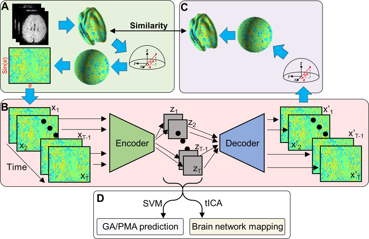
Variational autoencoder (VAE) and its application on fetal–neonatal functional magnetic resonance imaging (fMRI) data.
(A) From volumetric fMRI patterns, 2D brain pattern is estimated via geometric reformatting. (B) Through the encoder and decoder of VAE, each brain pattern is compressed to latent variable z and reconstructed to x’. (C) Reconstructed 2D image is re-shaped into cortical space through the inverse reformatting step. (D) Latent representations estimated by VAE are used as features of different analysis.
Figure 2
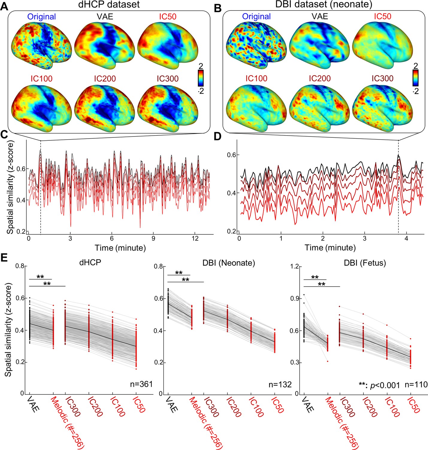
Variational autoencoder (VAE) represented fetal–neonatal functional magnetic resonance imaging (fMRI) patterns better than linear counterparts.
Compared to linear spaces defined by group independent component analysis (IC50, IC100, IC200, and IC300), VAE shows the best reconstruction performance on both Developing Human Connectome Project (dHCP) (A, C) and Developing Brain Institute (DBI) datasets (B, D), at the individual level and at the group level (E). **p<0.001, Bonferroni-corrected.
Figure 3
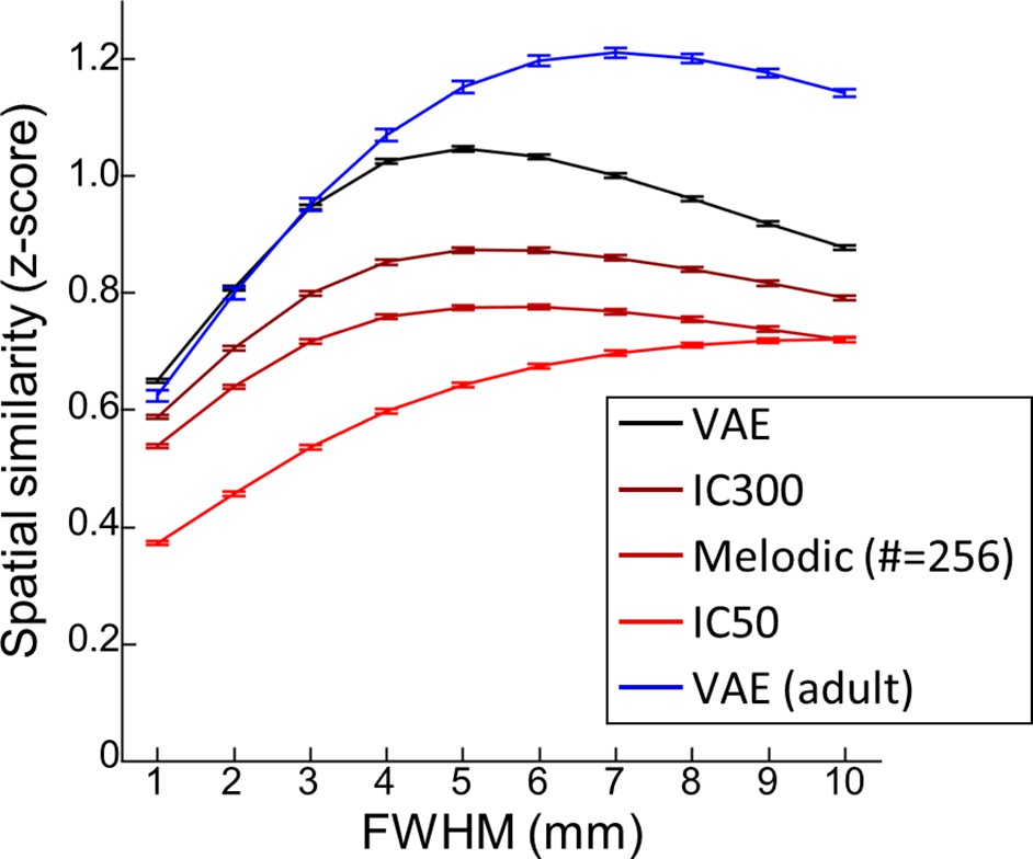
Smoothing effect of variational autoencoder (VAE) and linear counterparts.
A function of the full-half-maximum-width (FWHM) (from 1 to 10 mm) used for spatial smoothing of Developing Brain Institute (DBI) neonate functional magnetic resonance imaging (fMRI) images. The error bar stands for the standard error of mean. n = 139.
Figure 4 with 3 supplements
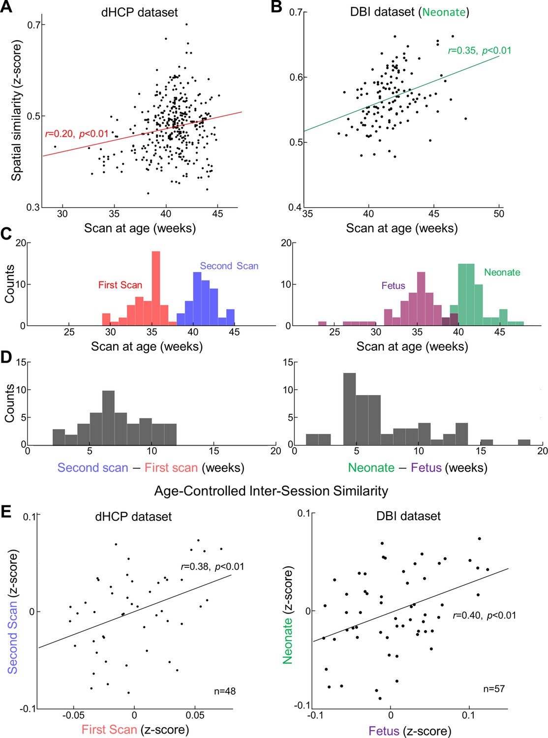
Reconstruction degree of functional magnetic resonance imaging (fMRI) patterns not only varies across different ages at scan but also is individual-specific.
Reconstruction degrees across individuals are positively correlated with their ages at scan for both datasets, Developing Human Connectome Project (dHCP) (A) and Developing Brain Institute (DBI) (B). In (B), each red dot stands for the outliers having >3 median absolute deviations away from the median. (C) Distributions of ages at repeated scans (left; dHCP dataset, first and second scans; right; DBI dataset, fetal and neonatal scans). (D) Distributions of inter-scan age difference, for dHCP (left) and DBI dataset (right). (E) Scatterplot of reconstruction degree between the first scan and (or fetal scan for DBI) and the second scan (or neonatal scan for DBI), after controlling the effect from ages at scan.
Figure 4—figure supplement 1
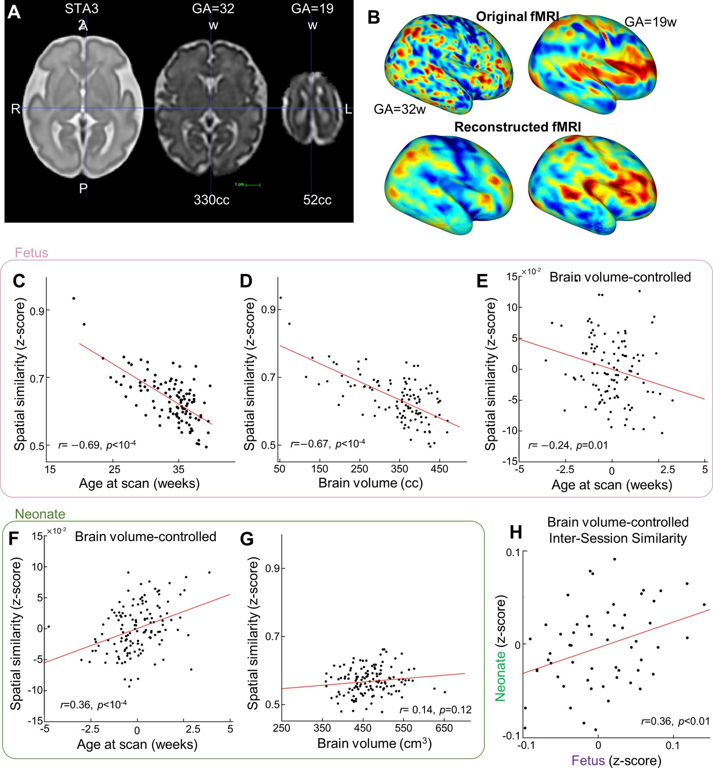
Smoothing effect of young fetal brain during projecting to standard brain template.
(A) The brain size of young fetus (GA=19 weeks) is only 52cc compared to fetus with GA=32 weeks. (B) Projecting fMRI activity of young fetus into the standard brain template induce more “balloon” effect compared to older fetuses (GA=32 week). (C) Variability of reconstruction degree of fMRI patterns across fetuses at different gestational ages. Red dots stand for the outliers having > 3 median absolute deviations away from the median. (D) Scatterplot between brain size and spatial similarity (n=108). (E) Partial regression plot between age at scan and reconstruction performance. (F-G) Same analysis as (B-C) but with neonate subjects. (H) Scatter plot between reconstruction degree at the fetal scan and reconstruction degree at the neonatal scan, after controlling the effect from brain size.
Figure 4—figure supplement 2
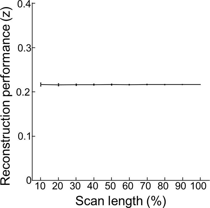
Age-dependency of reconstruction performance is not driven by scan length.
Figure 4—figure supplement 3
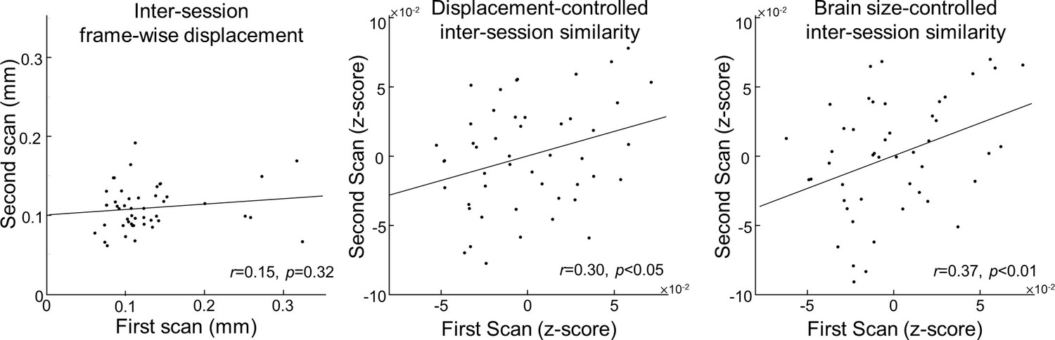
Reconstruction variability among individuals is not related to head motion artifact.
(Left) Scatter plot of average frame-wise displacement degree between repeated scans in dHCP dataset. After controlling the effect from motion artifact (Middle) or brain size (Right), reconstruction degree at the first scan is still significantly and positively correlated with reconstruction degree at the second scan.
Figure 5
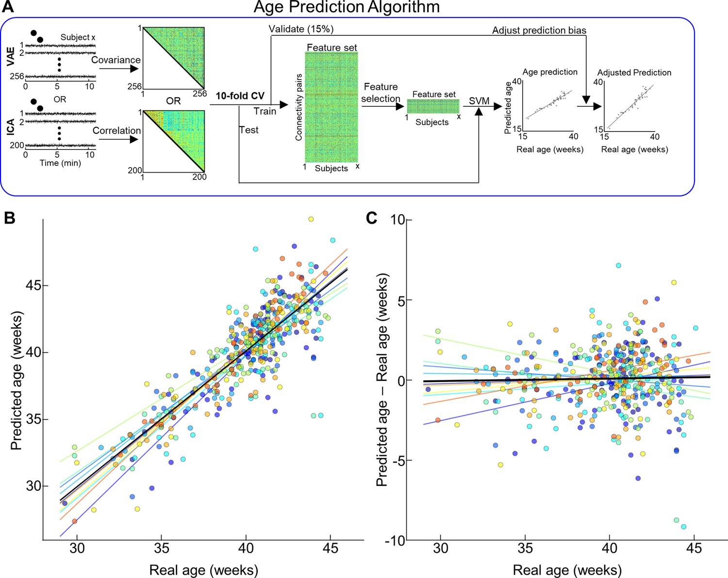
Age prediction based on different latent representations of neonates in the Developing Human Connectome Project (dHCP) dataset.
(A) Illustration of age prediction algorithm. (B) Scatterplot between actual age and predicted age. (C) Distribution of prediction error across age at scan. (B, C) Different colors stand for the prediction age from different folds. Lines with different colors stand for the optimal fit. Black line is the optimal fit for whole samples.
Figure 6
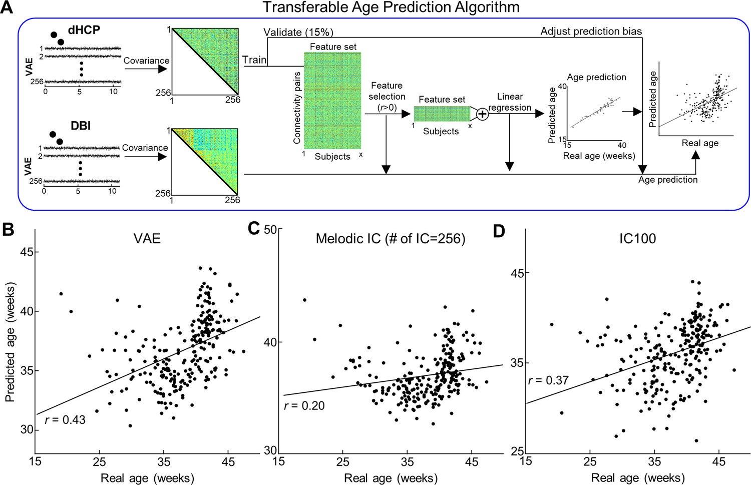
Cross-center age prediction algorithm using different latent representations.
(A) Illustration of transferable age prediction algorithm. (B–D) Scatterplot between actual age and predicted age using different latent representations. Each red dot stands for the outliers having >3 median absolute deviations away from the median reconstruction performance.
Figure 7 with 5 supplements
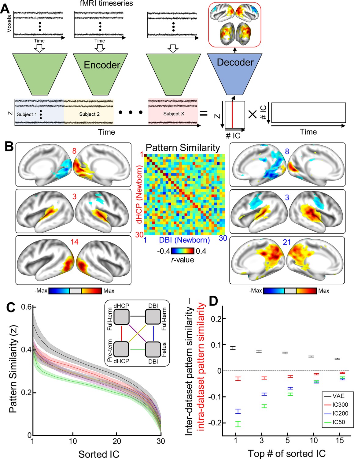
Mapping resting-state functional brain networks of fetuses and neonates using variational autoencoder (VAE).
(A) Illustration describing how to map functional brain networks using the VAE. (B) Example of neonatal cortical networks estimated from the Developing Human Connectome Project (dHCP) dataset (left) or the Developing Brain Institute (DBI) dataset (right). The order of estimated independent latent variables is sorted by their absolute pattern similarity across different datasets (center). Each map is thresholded at the level of <15% of maximal absolute value. (C) Pattern similarities across different datasets and/or different age groups (coded as lines with different colors; right panel) are plotted. Shades and line stand for the standard deviation and mean similarity across 100 IC results with different initializations. (D) The difference between inter-dataset pattern similarity (neonate in DBI vs. dHCP) and intra-dataset pattern similarity (neonate vs. preemie in dHCP). The similarity was measured by averaging top 1–15 of sorted IC. Error bar stands for the standard deviation.
Figure 7—figure supplement 1
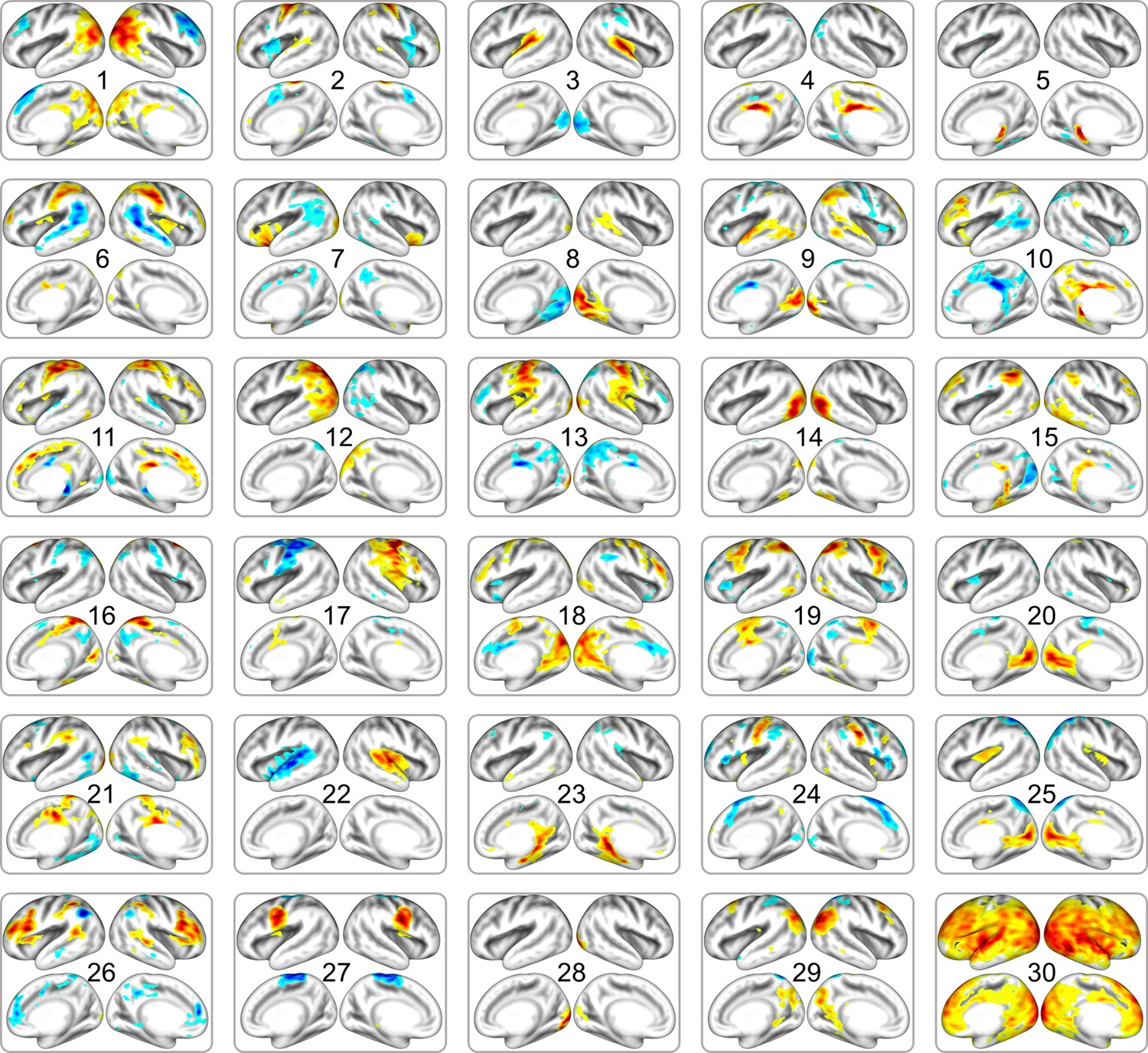
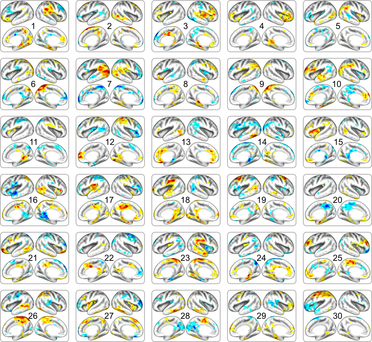
Full list of neonatal cortical networks estimated from dHCP dataset.
The order of estimated independent latent variables is sorted by their absolute scale of pattern similarity to DBI dataset. Each map is thresholded at the level of < 15% of maximal absolute value.
Figure 7—figure supplement 2
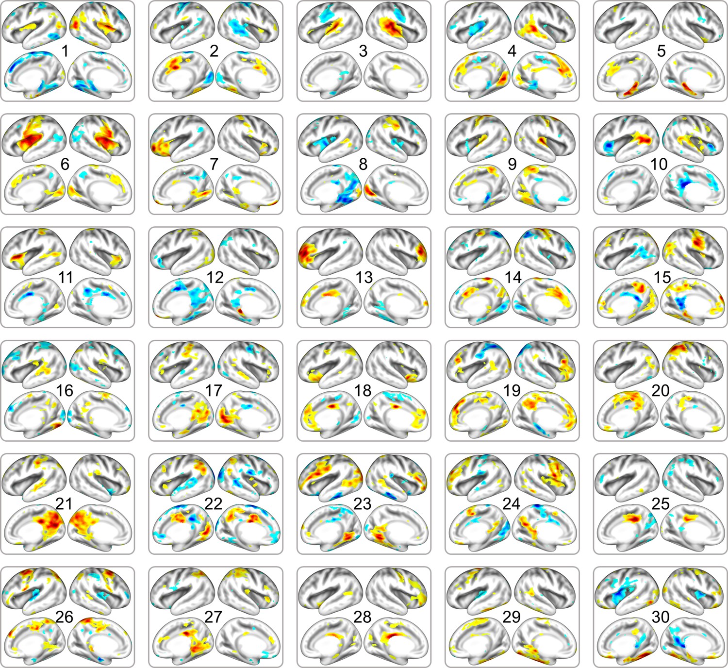
Full list of neonatal cortical networks estimated from DBI dataset.
The order of estimated independent latent variables is sorted by their absolute scale of pattern similarity to dHCP dataset. Each map is thresholded at the level of < 15% of maximal absolute value.
Figure 7—figure supplement 3

Full list of cortical networks of preterm babies estimated from dHCP dataset.
The order of estimated independent latent variables is sorted by their absolute scale of pattern similarity to fetal group of DBI dataset. Each map is thresholded at the level of < 15% of maximal absolute value.
Figure 7—figure supplement 4
Full list of fetal cortical networks estimated from DBI dataset.
The order of estimated independent latent variables is sorted by their absolute scale of pattern similarity to DBI dataset. Each map is thresholded at the level of < 15% of maximal absolute value.
Figure 7—figure supplement 5
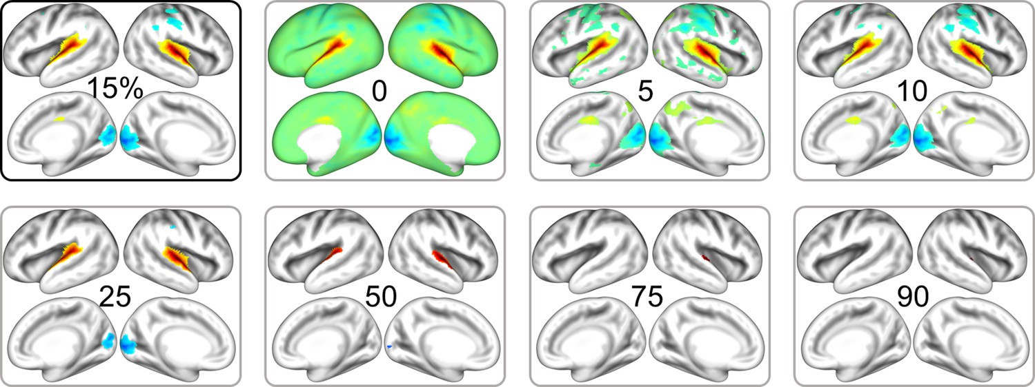
Cortical pattern of IC3 in the neonatal dHCP dataset.
Cortical maps are thresholded at varying level of maximal absolute value.
Figure 8 with 2 supplements
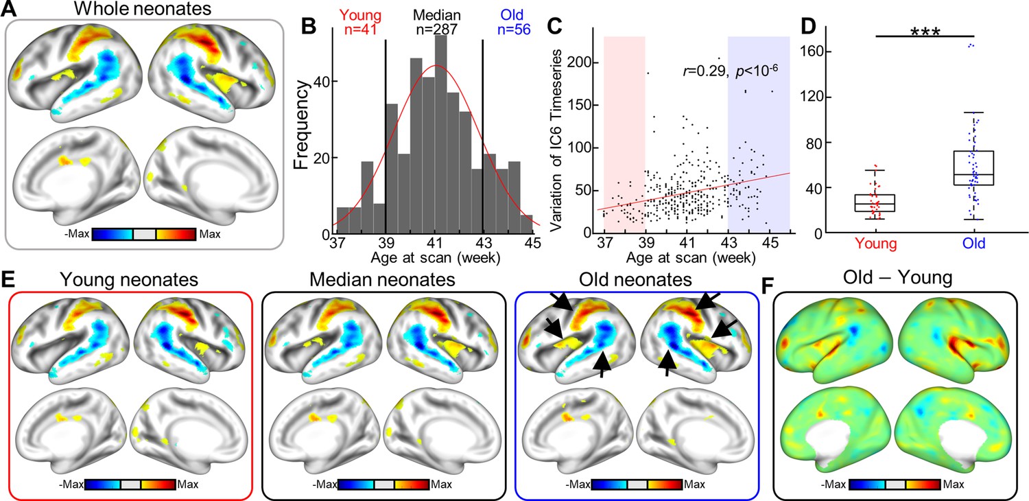
Between-group differences in resting-state functional brain networks using variational autoencoder (VAE).
(A) The cortical network represents the sixth independent component (IC6) derived from all neonates of the Developing Human Connectome Project (dHCP). (B) The distribution of age at scan for the neonate cohort (n = 384). Based on the age distribution, the cohort was divided into three groups; young, median, and old groups. (C) Scatterplot between age at scan (x-axis) and IC6 timeseries variance. Each dot represents a subject; n = 384. (D) Variance boxplot in young (postmenstrual age [PMA] at scan 39 wk) and old groups (PMA at scan 43 wk) of the dHCP dataset. ***p<10–8. (E) Cortical networks in different age groups using dual-regression method. Inset arrows point to brain regions having different activation levels in older group compared to younger group. (F) Difference between two age groups; subtraction between groups is done at the latent space, followed by projection to the cortical surface.
Figure 8—figure supplement 1
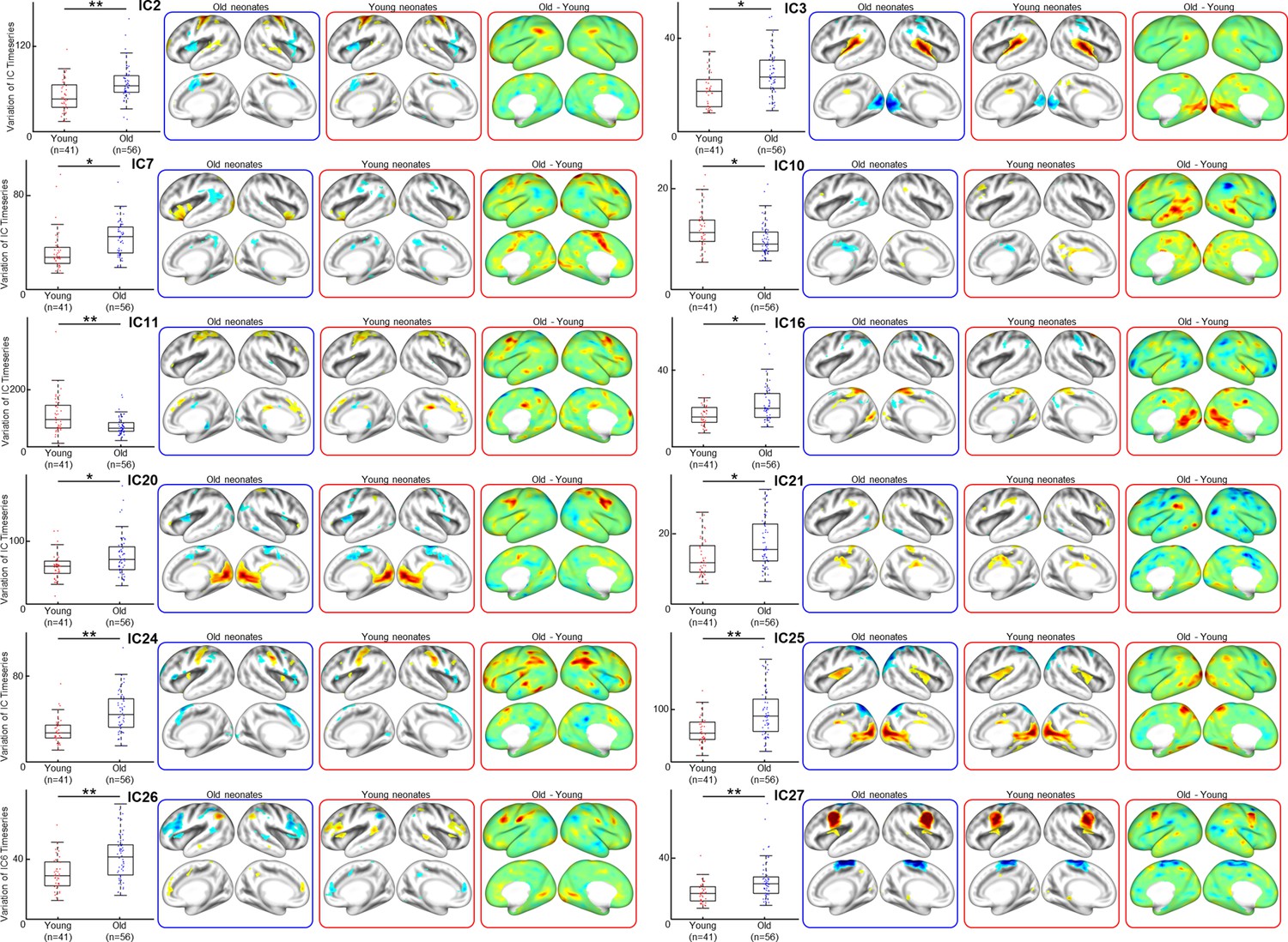
Differences in resting-state functional brain networks (FBN) between young and old neonates.
Visualization of distinct FBNs showing age-related difference. From left to right: variance between young (PMA at scan 39 weeks)- and old group (PMA at scan 43 weeks) of the dHCP dataset, the cortical network representing different age groups, and difference between two age groups.
Figure 8—figure supplement 2
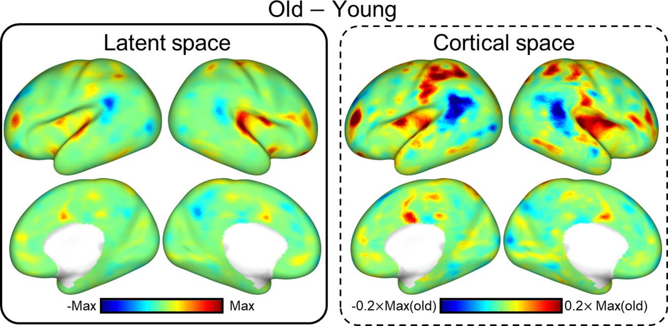
Group-wise difference in resting-state functional brain networks using VAE.
Difference between two age groups. subtraction between groups is done at the latent surface, followed by the projection to the cortical surface (left) or at the cortical space (right).
Tables
Table 1
Comparison of age prediction performance in Developing Human Connectome Project (dHCP) dataset using different latent representations.
RMSE: root mean squared error; MAE: mean absolute error; R2: explained variance; VAE: variational autoencoder; ICA: independent component analysis. Red highlight indicates the best performance among different latent representation methods.
| Representationmethod | RMSE(mean ± SD) | MAE | R2 | Correlation |
|---|---|---|---|---|
| VAE (N = 256) | ||||
| Cortical parcel (N = 360) | 2.35 ± 0.08*** | 1.85 ± 0.07*** | 0.65 ± 0.01*** | 0.80 ± 0.02*** |
| IC50 | 2.88 ± 0.15*** | 2.28 ± 0.12*** | 0.55 ± 0.02*** | 0.73 ± 0.03*** |
| IC100 | 2.67 ± 0.11*** | 2.12 ± 0.09*** | 0.59 ± 0.02*** | 0.76 ± 0.03*** |
| IC200 | 2.31 ± 0.09*** | 1.83 ± 0.07*** | 0.65 ± 0.01*** | 0.80 ± 0.02*** |
| IC300 | 2.43 ± 0.09*** | 1.94 ± 0.07*** | 0.63 ± 0.01*** | 0.79 ± 0.02*** |
| Melodic ICA (N = 256) | 2.23 ± 0.08*** | 1.76 ± 0.07*** | 0.67 ± 0.01*** | 0.81 ± 0.02*** |
| ***: Bonferroni-corrected p<10–4; compared to VAE. | ||||
Table 2
Comparison of age prediction performance in Developing Brain Institute (DBI) dataset using different latent representations.
RMSE: root mean squared error; MAE: mean absolute error; R2: explained variance; VAE: variational autoencoder; ICA: independent component analysis. Red highlight indicates the best performance among different latent representation methods.
| Representationmethod | RMSE(mean ± SD) | MAE | R2 | Correlation |
|---|---|---|---|---|
| VAE (N = 256) | ||||
| Cortical parcel (N = 360) | 4.55 ± 0.27*** | 3.64 ± 0.22*** | 0.58 ± 0.01*** | 0.73 ± 0.02*** |
| IC50 | 5.80 ± 0.52*** | 4.65 ± 0.43*** | 0.48 ± 0.02*** | 0.65 ± 0.04*** |
| IC100 | 5.74 ± 0.33*** | 3.78 ± 0.28*** | 0.57 ± 0.02*** | 0.73 ± 0.04*** |
| IC200 | 5.05 ± 0.36*** | 3.97 ± 0.29*** | 0.54 ± 0.02*** | 0.70 ± 0.03*** |
| IC300 | 4.82 ± 0.33*** | 3.79 ± 0.27*** | 0.57 ± 0.02*** | 0.72 ± 0.03*** |
| Melodic ICA (N = 256) | 4.24 ± 0.32*** | 3.33 ± 0.27*** | 0.62 ± 0.01*** | 0.76 ± 0.03*** |
| ***: Bonferroni-corrected p<10–4; compared to VAE. | ||||
Table 3
Cross-center generalizability of age prediction performance under different latent representations.
RMSE: root mean squared error; MAE: mean absolute error; VAE: variational autoencoder; ICA: independent component analysis. Red highlight indicates the best performance among different latent representation methods.
| Representationmethod | RMSE | MAE | vs. VAE (MAE) |
|---|---|---|---|
| VAE (N = 256) | |||
| Cortical parcel (N = 360) | 12.82 ± 15.38 | 12.06 ± 15.35 | p<10–6 |
| IC50 | 5.67 ± 0.54 | 4.46 ± 0.54 | p<10–6 |
| IC100 | 5.58 ± 0.92 | 4.46 ± 0.85 | p<10–6 |
| IC200 | 5.72 ± 0.89 | 4.75 ± 0.83 | p<10–6 |
| IC300 | 5.68 ± 0.98 | 4.71 ± 0.93 | p<10–6 |
| Melodic ICA (N = 256) | 5.78 ± 1.62 | 4.72 ± 1.60 | p<10–6 |
Additional files
-
MDAR checklist
- https://cdn.elifesciences.org/articles/80878/elife-80878-mdarchecklist1-v2.pdf
-
Supplementary file 1
Supplementary tables.
(a) Preprocessing steps for the DBI and dHCP datasets. (b) Age prediction performance in separate age groups of DBI dataset using different latent representations.
- https://cdn.elifesciences.org/articles/80878/elife-80878-supp1-v2.docx
Download links
A two-part list of links to download the article, or parts of the article, in various formats.
Downloads (link to download the article as PDF)
Open citations (links to open the citations from this article in various online reference manager services)
Cite this article (links to download the citations from this article in formats compatible with various reference manager tools)
Toward a more informative representation of the fetal–neonatal brain connectome using variational autoencoder
eLife 12:e80878.
https://doi.org/10.7554/eLife.80878


