Flexible specificity of memory in Drosophila depends on a comparison between choices
- HHMI Janelia Research Campus, United States
- The Solomon H. Snyder Department of Neuroscience, Johns Hopkins University School of Medicine, United States
- Aix-Marseille Univ, Université de Toulon, CNRS, CPT (UMR 7332), Turing Centre for Living Systems, France
Figures
Figure 1 with 1 supplement
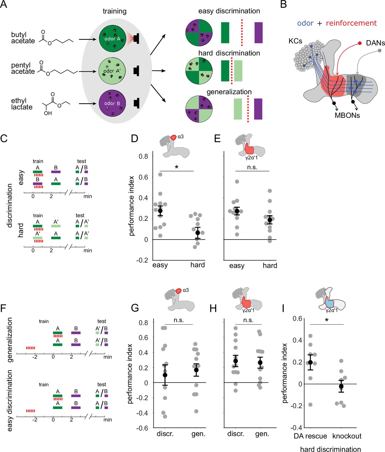
A single set of changed synapses can result in generalization or discrimination.
(A) Left: Chemical structures of the three odors used in the study, the similar odors butyl acetate (BA) and pentyl acetate (PA) and the dissimilar odor ethyl lactate (EL). Middle: During training the similar odors are interchangeably used as the odors that are paired (A) or unpaired (A’) with optogenetic reinforcement (LED). Right: Trained flies are then given one of three different choices between odors in opposing arena quadrants. These choices represent the three kinds of tasks used here to study memory specificity. Performance index measures the bias in the distribution of flies across the different quadrants (see Methods). The circles depict fly population behavior in our arenas and the vertical bars depict stimulus choices. The dashed, red line depicts the discrimination boundary in each choice. This boundary shifts relative to the light-green stimulus, depending on the options. (B) Mushroom body learning schematic. KCs activated by an odor (blue) form synapses on MBONs in two compartments (red and gray shading). Reinforcement stimulates the DAN projecting to one compartment (red) leading to synaptic depression. (C) Behavior protocols for discrimination tasks at two levels of difficulty. Colored bars represent odor delivery periods, red dashes indicate LED stimulation for optogenetic reinforcement. A represents the paired odor, A’ the similar odor and B the dissimilar odor. (D) Significantly lower performance on the hard discrimination task with reinforcement to α3 (p=0.007, n=12). Flies received 10 cycles of training and were tested for memory 24 hours later. CsChrimson-mVenus driven in DAN PPL1-α3 by MB630B-Gal4. (E) No significant difference in performance on easy versus hard discrimination with reinforcement to γ2α’1 (p=0.08, n=12 reciprocal experiments). Flies received three cycles of training and were tested for memory immediately after. CsChrimson-mVenus driven in DAN PPL1 γ2α’1 by MB296B-Gal4. (F) Behavior protocol for generalization. Scores here are compared to a control protocol where light stimulation is not paired with odor presentation in time. (G) No significant difference in performance on generalization and easy discrimination with reinforcement to α3 (p=0.84, n=12). Flies received 10 cycles of training and were tested 24 hr later. (H) No significant difference in performance on generalization and easy discrimination with reinforcement to γ2α’1 (p=0.89, n=12 unpaired control performance scores). Flies received three cycles of training and were tested immediately after. (I) Rescue of the dopamine biosynthesis pathway in DAN PPL1-γ2α’1 is sufficient for performance on the hard discrimination task (p=0.04, n=8). Black circles and error bars are mean and SEM. Statistical comparisons made with an independent sample Wilcoxon rank sum test.
Figure 1—figure supplement 1
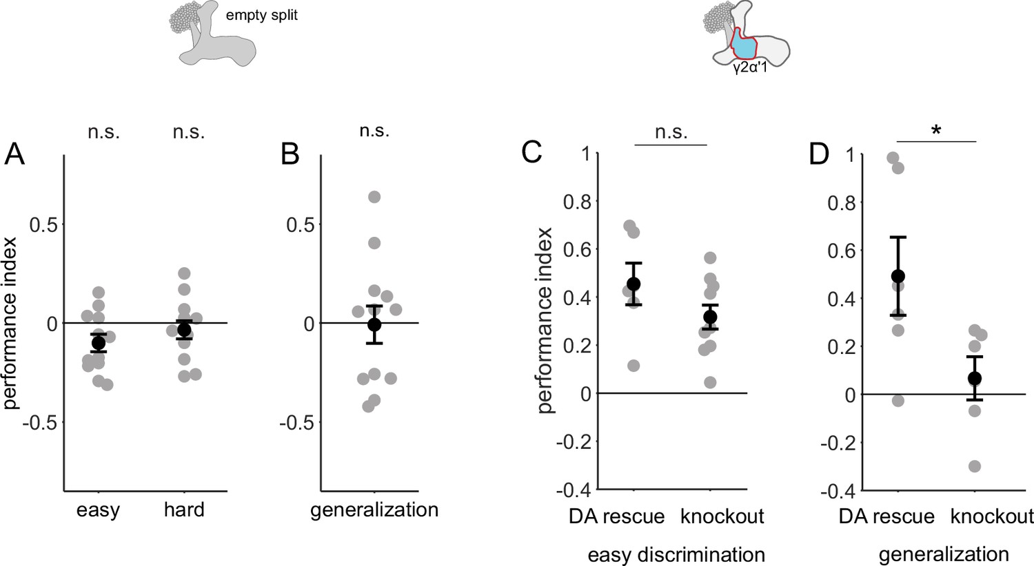
Control behavior experiments.
(A and B) Flies with Chrimson driven by an empty split-Gal4 driver, i.e. with no Chrimson expression did not learn any of the tasks. Performance indices not significantly different from 0 (n=12, p=0.052, 0.38 and 0.91 and for easy, hard discrimination and generalization; single-sample, Wilcoxon signed rank test). (C) Flies with no expression of dopamine in their nervous systems (knockout) are capable of performing the easy discrimination task as well as flies with dopamine rescued in DAN PPL1-γ2α’1 (rescue n=6, knockout n=12, p=0.22, Wilcoxon rank sum test). (D) Flies with dopamine expression rescued in DAN PPL1-γ2α’1 alone are capable of generalization, while flies with dopamine knockout are not (n=6 for rescue and knockout, p=0.041, Wilcoxon rank sum test).
Figure 2 with 1 supplement
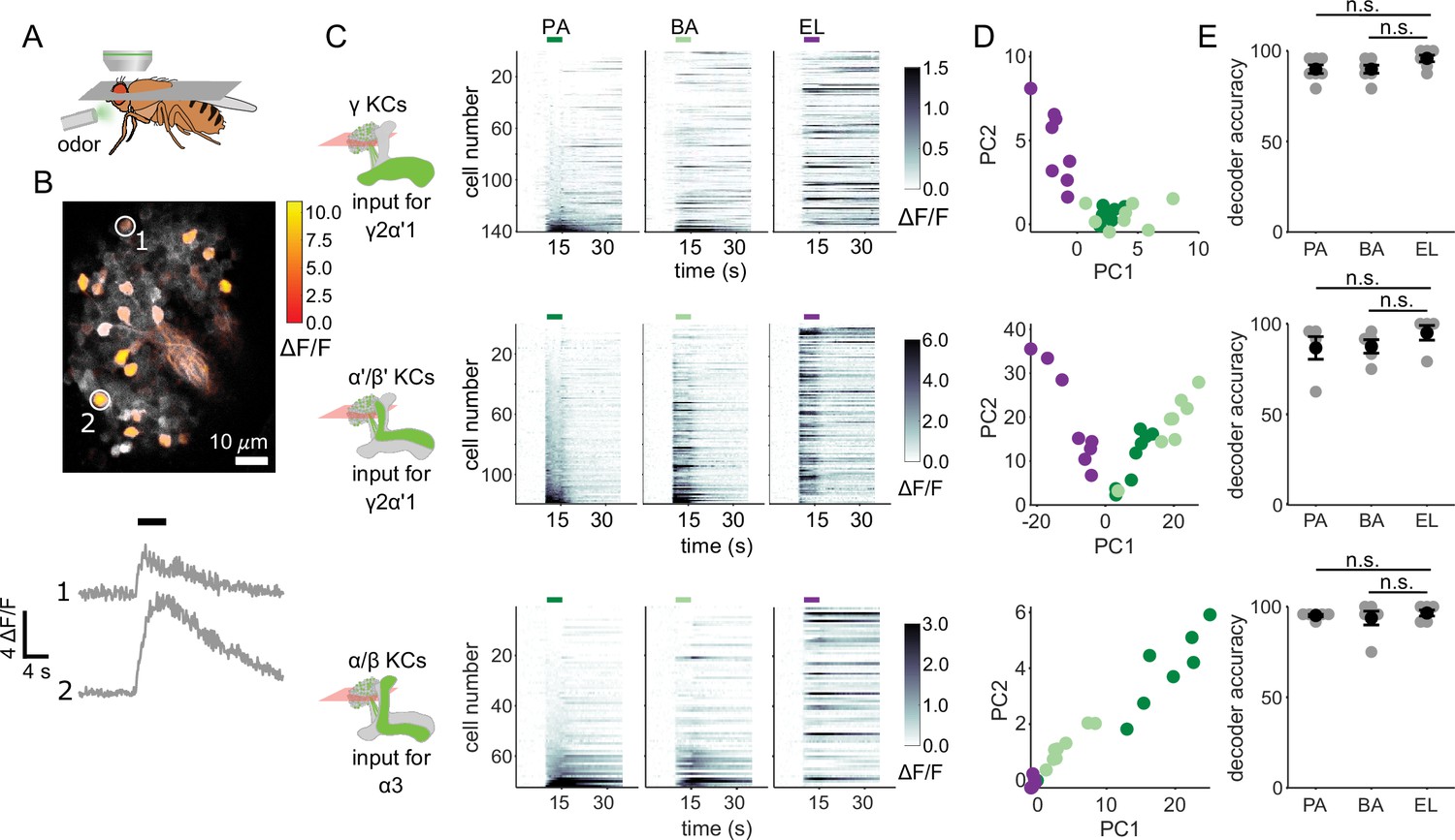
KC responses to single odor pulses contain enough information to discriminate similar odors.
(A) Schematic of in vivo imaging preparation. (B) Example single-trial odor response patterns in α/β KCs. ΔF/F responses (color bar) are shown overlaid on baseline fluorescence (grayscale). Numbered circles indicate cells for which ΔF/F traces are plotted below. Black bar indicates odor delivery. (C) ΔF/F responses of different KC subtypes to the three odors used in this study. Rows show responses of individual KCs, averaged across trials, sorted by responses to PA. GCaMP6f was driven in γ KCs by d5HT1b-Gal4, in α’/β’ KCs by c305a-Gal4 and in α/β KCs by c739-Gal4. Colored bars above plots indicate the odor delivery period. (D) Odor response patterns for the same example flies as in C, projected onto the first two principal component axes to show relative distances between representations for the different odors. (E) Decoder prediction accuracies, plotted across flies. Each gray circle is the accuracy of the decoder for one fly for a given odor, averaged across all trials. Black circles and error bars are means and SEM. For γ KCs (top), decoder accuracies for PA (n=7 flies, p=0.06) and BA (p=0.08) were not significantly different from EL accuracy. This was also true for α’/β’ KCs (middle, n=5 flies, p=0.13 for the PA-EL comparison and p=0.13 for BA-EL) and α/β KCs (bottom, n=6 flies, p=0.63 for PA-EL and p=0.73 for BA-EL). All statistical testing was done with a paired-sample, Wilcoxon signed rank test with a Bonferroni-Holm correction for multiple comparisons. (C,D) In this figure, each shade of green denotes one of the two similar odor chemicals. But in subsequent figures, the darker shade represents the odor paired with reinforcement and the lighter shade, the unpaired, similar odor. In the reciprocal design we use, each of the odor chemicals is the paired odor in half the experimental repeats.
Figure 2—figure supplement 1
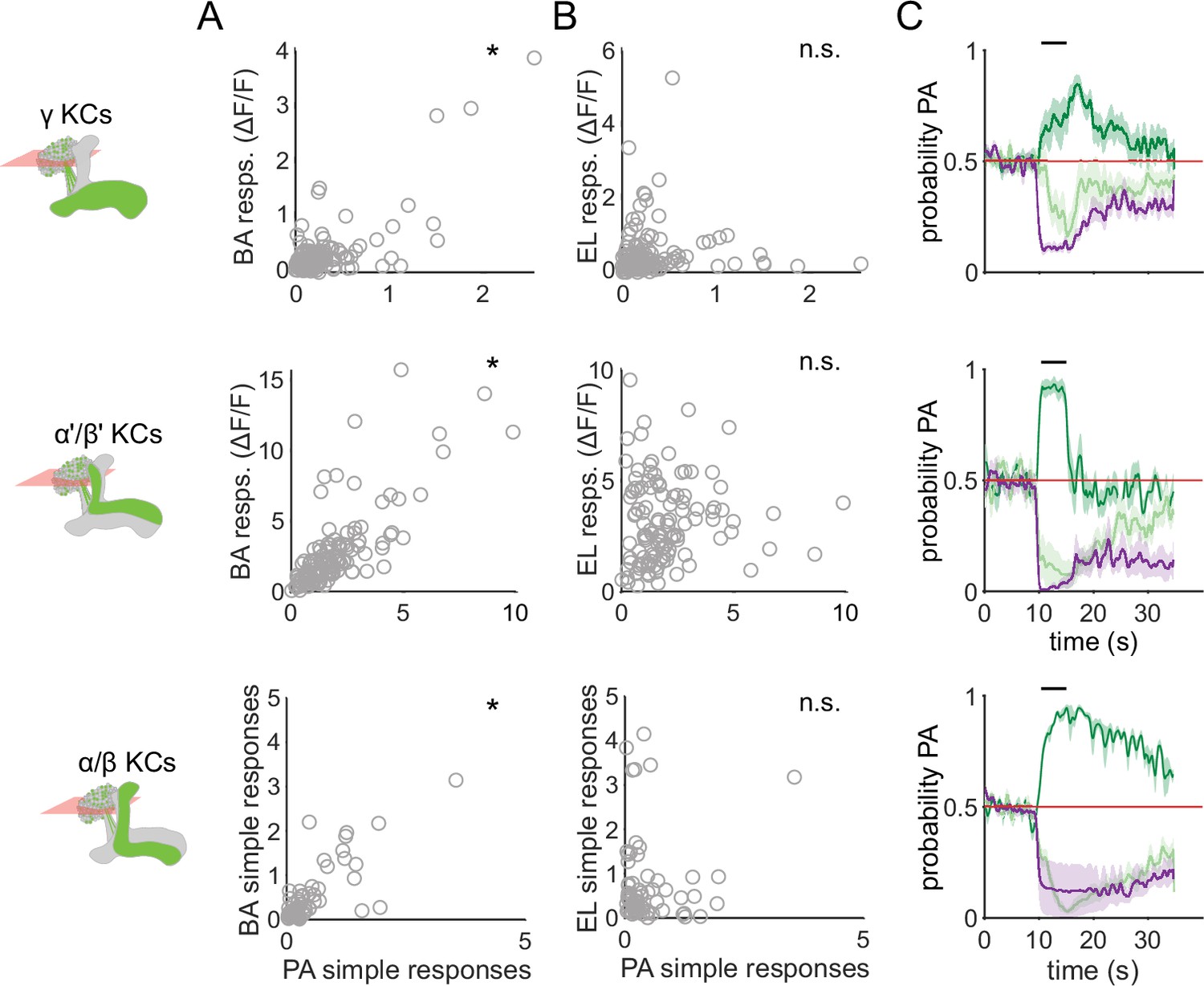
Similar odors have similar KC response patterns.
(A) Scatter plots showing the similarity of the mean odor response of individual KCs to the two similar odors PA and BA. Correlations were significant across all three KC subtypes (γ KCs: Pearson’s correlation coefficient, r=0.74, p<0.001; α’/β’ KCs: r=0.76, p<0.001; α/β KCs: r=0.63, p<0.001). (B) Scatter plots as in A, but for dissimilar odors PA and EL. No significant correlations in this case (γ KCs: r=0.044, p=0.60; α’/β’ KCs: r=0.06, p=0.55; α/β KCs: r=–0.04, p=0.77). (C) Decoder-predicted probability that the odor delivered was PA, plotted against time. Prediction for trials on which PA was delivered are plotted in dark green, BA – light green and EL – purple. The red line indicates the positive prediction threshold. The black bar at the top indicates odor delivery period. Solid lines are mean, and shading indicates SEM. Probabilities are plotted for the same example fly as in Figure 2C for each KC type.
Figure 3
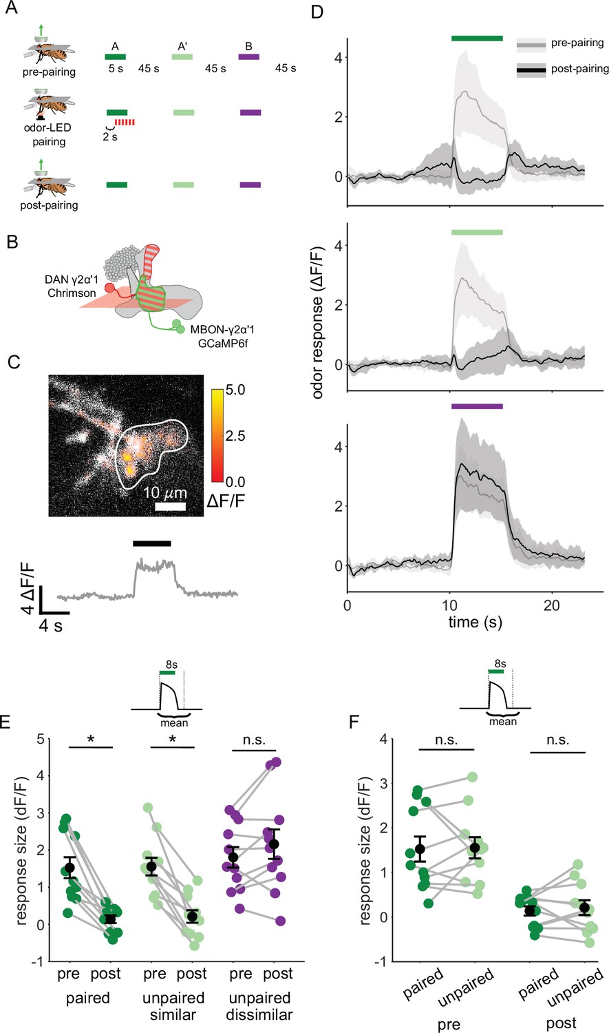
Plasticity in MBON γ2α’1 is not sufficiently odor specific for hard discrimination.
(A) Stimulus protocol for on-rig, in vivo training. Plasticity in MBON γ2α’1 was assessed by imaging pre- and post-pairing with optogenetic reinforcement via DAN PPL1-γ2α’1. There was no imaging during the pairing itself. Colored bars represent 5 s odor delivery (dark green: odor A paired; light green: odor A’ unpaired similar; purple: odor B unpaired dissimilar). PA and BA were used as the paired odor for every alternate fly. (B) Schematic of experimental design. Expression of GCaMP6f in MBON-γ2α’1 driven by MB077B-Gal4 and Chrimson88-tdTomato in DAN PPL1-γ2α’1 by 82C10-LexA. Imaging plane in the γ lobe as indicated. (C) Example MBON-γ2α’1 single-trial odor response. ΔF/F responses (color bar) are shown overlaid on baseline fluorescence (grayscale). White ROI indicates neuropil region for which a single-trial ΔF/F trace is plotted below. Black bar indicates odor delivery. (D) MBON γ2α’1 ΔF/F response traces pre- (grey) and post- (black) pairing (mean +- SEM, n=11 flies). Bars indicate 5 s odor delivery period; colors correspond to odor identities in a. (E) Response sizes pre- and post-pairing show a reduction for both paired (dark green, p=0.001), and similar unpaired (light green, p=0.001) odors but not the dissimilar odor (purple, p=0.18). Response amplitude calculated as mean ΔF/F over an 8 s window starting at odor onset (inset). Connected circles indicate data from individual flies. (F) Data as in E, re-plotted to compare responses to the paired odor with responses to the unpaired, similar odor before and after training. Response sizes were not significantly different pre- (p=0.77) or post-pairing (p=0.77). Statistical comparisons made with the paired sample Wilcoxon signed rank test, with a Bonferroni Holm correction for multiple comparisons.
Figure 4 with 4 supplements
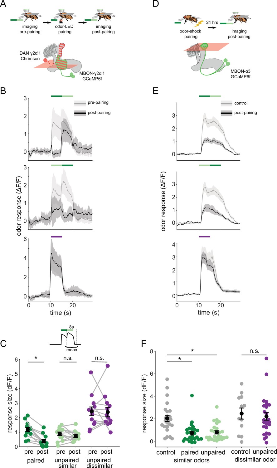
Odor transitions enable discrimination by MBON-γ2α’1 but not MBON-α3.
(A) Schematic of experimental design to assess plasticity in MBON-γ2α’1. Protocol was identical to Figure 3A, except odor transitions were used as pre- and post-pairing test stimuli to mimic odor boundaries from the behavioral arena. See Figure 4—figure supplement 2A for the detailed protocol. (B) MBON-γ2α’1 ΔF/F response time courses pre- (gray) and post- (black) pairing to different odor transitions (mean +- SEM, n=13 flies). Colored bars indicate timing of odor delivery, dark green: paired odor, light green: unpaired, similar odor, purple: dissimilar odor. Schematic of the corresponding fly movement in the behavior arena at left. (C) Response sizes in MBON-γ2α’1 pre- and post-pairing for the second odor in the transition. Responses calculated as mean over an 8 s window starting at the onset of the second odor (inset). Responses when the paired odor is second are significantly reduced after pairing (dark green n=13 flies, p<0.001). By contrast there is no significant reduction when the unpaired similar odor comes second (light green p=0.376). The dissimilar odor control showed no significant change (purple, p=1). Connected circles indicate data from individual flies. (D) Schematic of experimental design for MBON-α3. Flies were trained by pairing odor with shock in a conditioning apparatus and odor responses were imaged 24 hr later. Plasticity was assessed by comparing responses against those from a control group of flies exposed to odor and shock but separated by 7 min. See Figure 4—figure supplement 2B for the detailed protocol. GCaMP6f was driven in MBON-α3 by MB082C-Gal4 (bottom). (E) MBON-α3 ΔF/F response traces as in B. Light gray traces are from control shock-exposed flies (n=12 flies), dark gray traces are from odor-shock paired flies (pooled n=14 PA-paired and n=12 BA-paired flies). Averaged control traces were pooled across trials where either PA or BA was the second odor in a transition. (F) Response sizes in MBON-α3 in control (gray) and trained flies (colored) for the second odor in the transition (computed as in C). Responses are significantly reduced in trained flies both when the paired odor is second (dark green, n=14 PA-paired and n=12 BA-paired flies pooled, p<0.001) and when the unpaired similar odor is second (light green, p<0.001). Responses to the dissimilar odor were not significantly different (purple, p=0.48). Plotted control responses were pooled across trials where PA or BA was the second odor in a transition. (C,F) Statistical comparisons for MBON-γ2α’1 made with the paired sample, Wilcoxon signed-rank test. For MBON-α3, where responses were compared across different flies, we used the independent samples Wilcoxon’s rank-sum test. p-values were Bonferroni-Holm corrected for multiple comparisons.
Figure 4—figure supplement 1
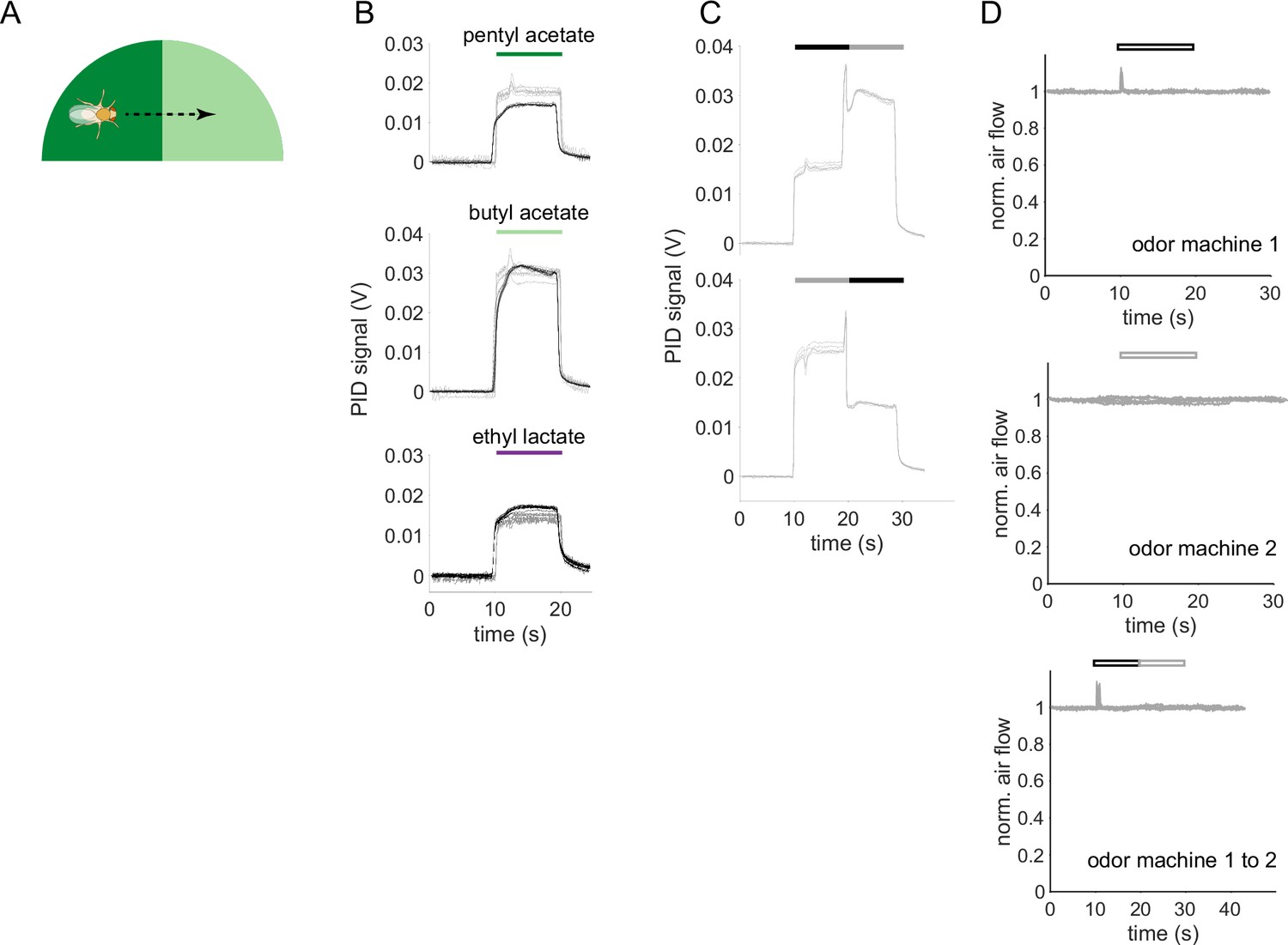
Time courses of odor delivery and air flow for odor pulses and odor transitions.
(A) Schematic showing a fly crossing a boundary between the paired and unpaired odor quadrants in the behavior arena. As the fly crosses the boundary, it experiences odors as a transition in time. (B) Photo-ionization detector (PID) signals for the odor stimuli used in this study. Single odor pulses from odor machine 1 shown in black (traces for five repeats overlaid) and pulses from odor machine 2 in gray. Note that at a given concentration in air, each odor-chemical can generate different ionization signal amplitudes. (C) PID traces for odor transitions PA to BA (top) and BA to PA (bottom). Throughout this study, the first odor pulse was always delivered by odor machine 1 and the second pulse by machine 2. (D) Hot-wire anemometer measurements of change in air velocity relative to steady-state flow. Top two panels are single stimulus pulses from each odor machine, bottom is for a transition stimulus. Hollow bars indicate that these measurements were taken without odorants in the airflow to avoid chemical interactions with the anemometer. Steady state flow rate as measured with a floating-ball flowmeter was 400 mL/min.
Figure 4—figure supplement 2
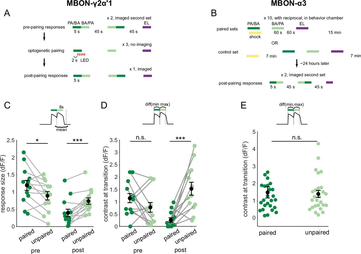
Contrast around odor transitions is high for MBON-γ2α’1 but not MBON-α3.
(A,B) Detailed schematics for training protocols used in Figure 4. (A) For MBON-γ2α’1, we imaged pre- and post-pairing responses to 5 s pulses of the two similar odors presented as transitions, and the dissimilar odor presented singly. Each pairing trial consisted of a single 5 s odor stimulus paired with 5 s of LED flashes, followed by 5 s presentations of the similar unpaired odor and the dissimilar odor, with 45 s in between each odor presentation. Pairing was repeated three times with 45 s between pairing trials. Each of the similar odors was paired with LED reinforcement for every alternate imaged fly as part of a reciprocal experiment design. (B) For MBON-α3, we only imaged post-pairing responses, 24 hr after odor-shock reinforcement. This is because learning is only expressed hours after reinforcement in this compartment. A pairing trial consisted of a single, 60 s odor presentation paired with shock, followed by 60 s presentations of the unpaired similar and dissimilar odors, with 60 s in between each odor presentation. Pairing was repeated 10 times, with 15 min between pairing trials. PA and BA were used as the paired odor alternate sets of flies as odor reciprocals. We could not measure the odor responses of flies before learning. So, we measured un-paired odor responses in flies that were exposed to shock and odor stimuli of equal durations, except with a 7-min interval between shock and the first odor stimulus in mock-pairing trials. These were the shock-exposed controls. (C) Same data as Figure 4C, quantifying responses to the second odor pulse, but re-plotted to compare responses to the paired odor with responses to the unpaired, similar odor before and after training. Pre-pairing, the responses to the paired odor were slightly but significantly higher (p=0.02), but post-pairing, responses to the unpaired similar odor were higher (p=0.004). (D) Contrast scores at the different odor transitions for MBON-γ2α’1 responses. Labels indicate the odor coming second in the transition. Contrast calculated as the difference between the maximum ΔF/F value during the second pulse and the minimum during the first pulse (inset). Pre-pairing, contrast was not different for the two kinds of transitions (p=0.19). Post-pairing contrast was higher for the transition to the unpaired, similar odor (p=0.001). Connected circles indicate data from individual flies. Statistical comparisons made using the paired sample Wilcoxon signed rank test with a Bonferroni Holm correction for multiple comparisons. (E) Contrast scores as D, for MBON-α3 responses in arena-trained flies. Contrast scores were not significantly different for the two directions of the transition (n=14 PA-paired and 12 BA-paired flies, pooled, p=0.86). Statistical comparison made with independent sample Wilcoxon’s rank-sum test, with Bonferroni-Holm corrections for multiple comparisons.
Figure 4—figure supplement 3
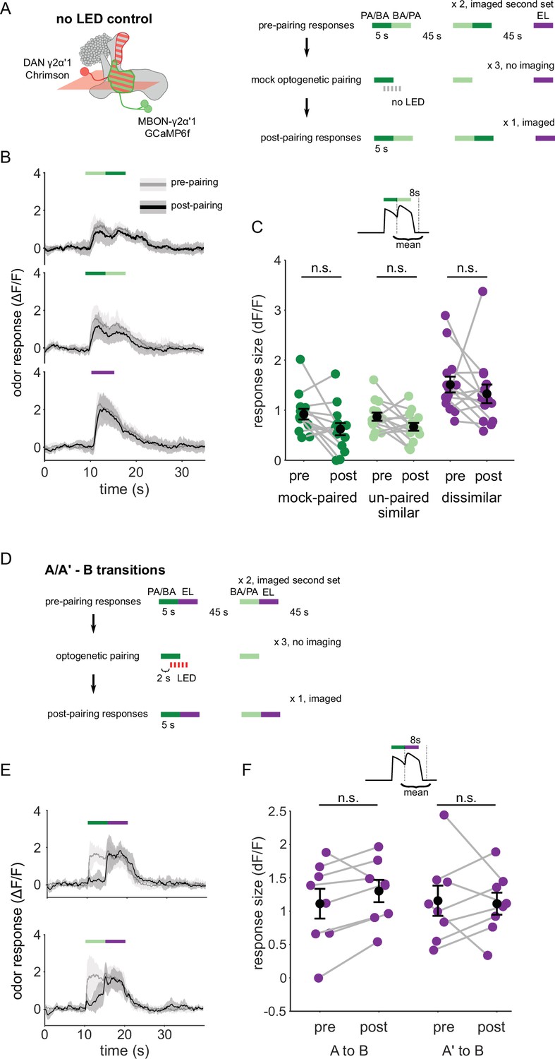
Observations from no-LED control training and odor transitions to the dissimilar odor.
(A) Protocol schematic. Same as in Figure 4—figure supplement 2A, except with no LED flashes in the training trials. (B) MBON-γ2α’1 ΔF/F response time courses to different odor transitions pre- (gray) and post- (black) no-LED control training (mean +- SEM, n=14 flies). Colored bars indicate timing of odor delivery, dark green: paired odor, light green: unpaired similar odor, purple: dissimilar odor. (C) Response sizes in MBON-γ2α’1 for the second odor in the transition with no-LED control training protocol. Response amplitude calculated as mean over an 8 s window starting at the onset of the second odor (inset). Responses are not significantly reduced for any stimulus (n=14 flies; paired odor: p=0.06; unpaired, similar odor p=0.17; dissimilar odor p=0.19). (D) Protocol schematic. Same as in Figure 4—figure supplement 2A, except with transitions from odors A or A’ to the dissimilar odor B. (E) MBON-γ2α’1 ΔF/F response time courses as in B, except for transitions from the paired odor or the similar, unpaired odor to the dissimilar odor. (F) Response sizes computed as in C, during the second, dissimilar odor pulse in each kind of transition stimulus plotted in E (n=8 flies, pared p=0.148, unpaired p=0.945).
Figure 4—figure supplement 4

PPL1-α3 split-LexA lines drive expression poorly.
(A) Maximum intensity z-projection image of GFP expression under MB630B split-Gal4 that was used to drive Chrimson in PPL1-α3 DANs for the behavior experiments in Figure 1. (B) Expression images for two split-LexA lines corresponding to MB630B.
Figure 5 with 1 supplement
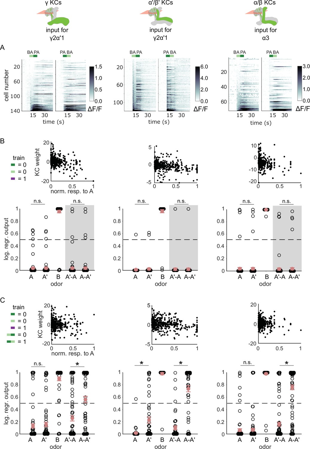
KC responses to odor transitions are not sufficient for hard discrimination.
(A) ΔF/F responses of different KC subtypes to odor transitions. Rows show responses of individual KCs, averaged across trials, sorted by responses to BA-PA. GCaMP6f was driven in γ KCs by d5HT1b-Gal4 (left), in α’/β’ KCs by c305a-Gal4 (middle) and in α/β KCs by c739-Gal4 (right). The odor delivery periods are indicated by colored bars at the top. (B) We fitted KC weights with logistic regression to give high or low outputs to odors consistent with measured MBON outputs (synaptic weight plots, black circles are individual fitted weights, pooled across flies). Individual logistic regression model outputs for held out test data for all types of odor stimuli are plotted in black. The gray background indicates that odor transition data was not part of the training set (n=96 models for γ, n=80 for α’/β’ and n=96 for α/β KCs, respectively), red circles and error bars are mean +/-SEM. The dashed, gray line at 0.5 indicates the logistic regression output threshold. Mean model outputs were below the decision threshold for A and A’ and were not significantly different (p=1 for γ, p=1 for α’/β’ and p=1 for α/β KCs, respectively), as was the case for A’-A and A-A’ (p=1 for γ, p=0.95 for α’/β’ and p=1 for α/β KCs, respectively). (C) Fitted weights and outputs for logistic regression models as in B, except that these were trained on single pulse as well as odor transitions. Average model outputs for A and A’ were below the decision threshold and were significantly different only for one KC sub-type (p=0.026 for γ, p<0.001 for α’/β’ and p=0.062 for α/β KCs, respectively). Mean outputs for A’-A were below the decision threshold, but outputs for A-A’ were above it and significantly different for all KC subtypes (p<0.001 for γ, p<0.001 for α’/β’ and p<0.001 for α/β KCs, respectively). All statistical comparisons were made with the Wilcoxon signed-rank test with a Bonferroni-Holm correction for multiple comparisons.
Figure 5—figure supplement 1
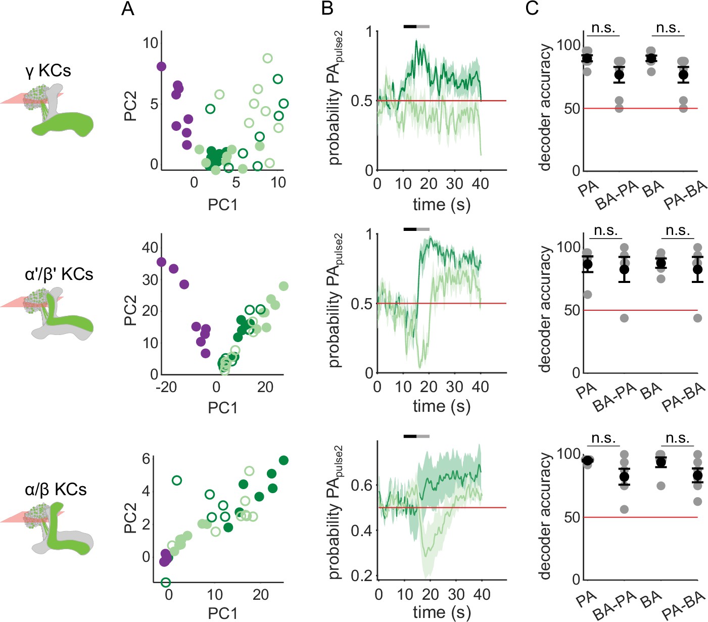
KC response patterns are similar for both isolated odor pulses and transitions.
(A) KC population odor responses for the same example flies as in Figure 2C, projected onto the first two principal component axes to show relative distances between representations for the different odors delivered as single pulses (filled circles) or as the second pulse in a transition (empty circles). (B) Decoder-predicted probability that the second odor in a transition was PA, plotted against time. Prediction for trials on which PA was the second pulse are plotted in dark green, and BA – light green. The red line indicates the positive prediction threshold. The black and gray bars at the top indicate the two odor pulse delivery periods. Solid lines are mean, and shading indicates SEM. Probabilities are plotted for the same example fly as in Figure 2C for each KC type. (C) Decoder prediction accuracies for odor transitions, plotted across flies. Each gray circle is the accuracy of the decoder for one fly for a given odor, averaged across all trials. Black circles and error bars are means and SEM. For γ KCs (top), decoder accuracies for PA (n=7 flies, p=0.098) and BA (p=0.047) were not significantly different from when they were delivered second in transitions. This was also true for α’/β’ KCs (middle, n=5 flies, p=0.817 for the PA v/s BA-PA comparison and p=0.94 for BA v/s PA-BA) and α/β KCs (bottom, n=6 flies, p=0.082 for PA v/s BA-PA and p=0.14 for BA v/s PA-BA). All statistical testing was done with a paired-sample, Wilcoxon signed rank test with a Bonferroni-Holm correction for multiple comparisons.
Figure 6 with 2 supplements
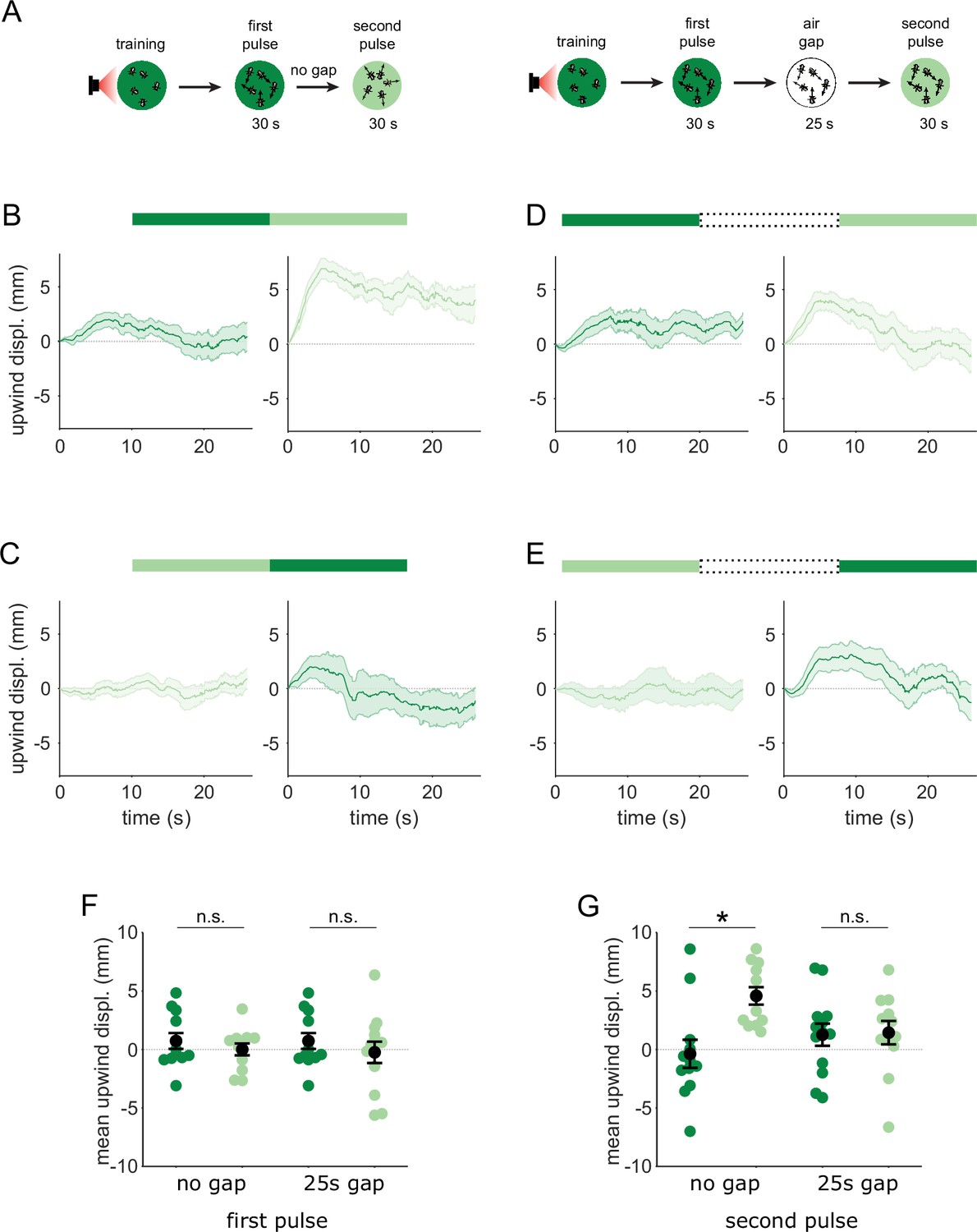
Flies are attracted to the unpaired odor only in transitions.
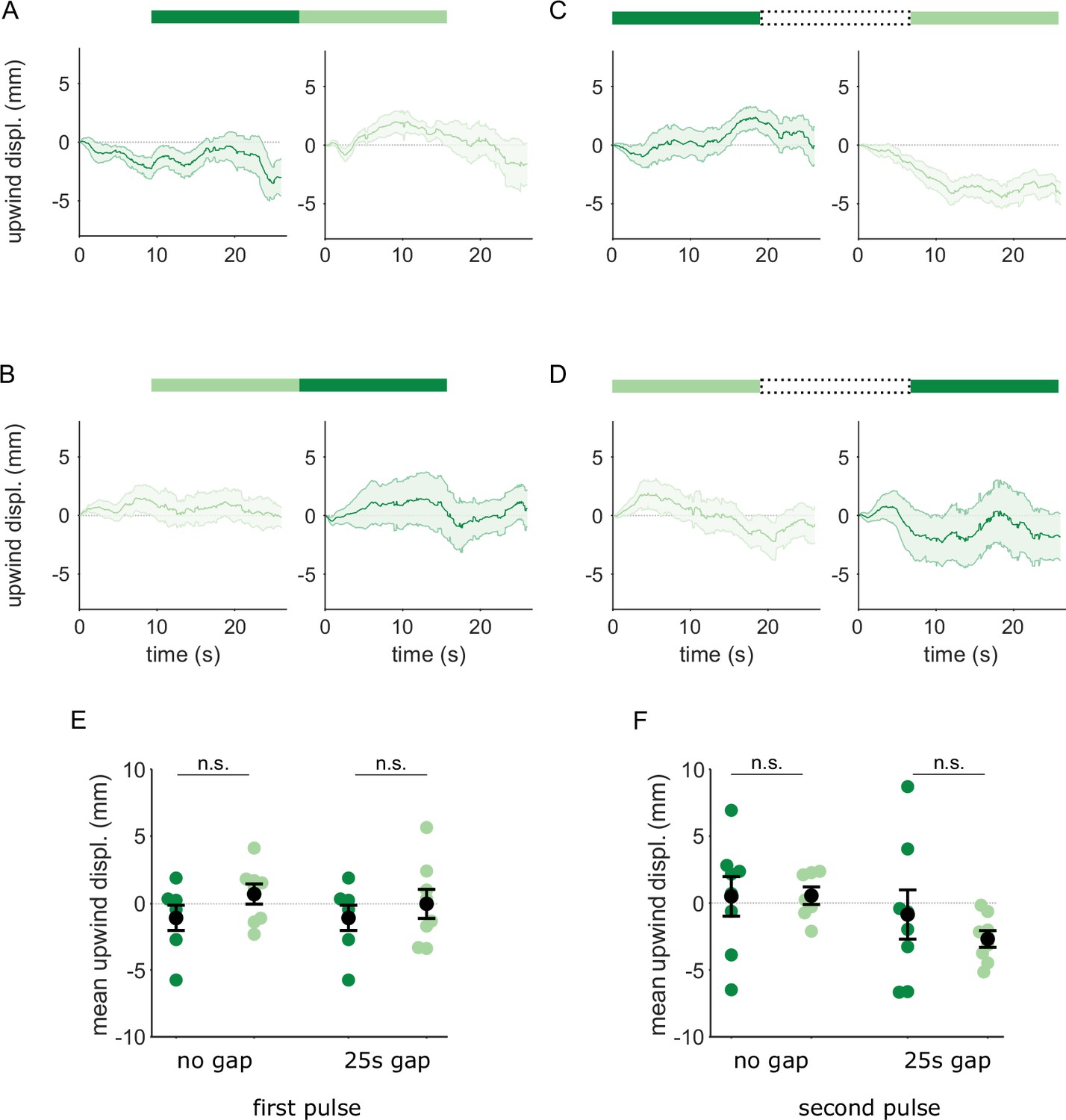
(A) Experimental strategy for measuring behavioral responses to odor transitions. Flies were trained by pairing one of the similar odors with optogenetic activation of DAN PPL1-γ2α’1. They were then tested with 30 s odor pulses presented either as direct transitions (left) or interrupted by a 25 s air period (right). Schematics illustrate A-A’ transitions but both sequences were tested, as indicated by the bars on top of panels B-E. (B) Upwind displacement during the first and second pulses of an A-A’ odor transition, as indicated by the green bars up top. This was computed as the increase in each fly’s distance from the arena center over the odor delivery period, then averaged across all flies in an arena (approximately 15 flies per arena). Traces in dark and light green are responses to A and A’ respectively. Plots are mean +/-SEM (n=12 arena runs for all stimulus types). (C) Upwind displacement for the reverse odor transition i.e. A’-A. (D) Upwind displacement for A-gap-A’ interrupted transition. (E) Upwind displacement for the reverse A’-gap-A interrupted transition. (F) Upwind displacement in response to the first odor pulse, averaged across flies in each arena experiment. Mean displacement was not significantly different between unpaired and paired odors for experiments with no gap (n=12, 12 experiments for paired and unpaired odors, p=0.70) and a 25 s gap (n=12, 13, p=0.40). (G) As in F except for responses to the second odor pulse. Displacement was significantly different for transitions with no gap between pulses (n=12, 12 experiments for paired and unpaired odors, p=0.004) but not different when transitions were interrupted by a 25 s gap (n=12, 13, p=0.85). Statistical comparisons in F and G were made with the independent-sample Wilcoxon rank sum test with a Bonferroni-Holm correction for multiple comparisons.
Figure 6—figure supplement 1
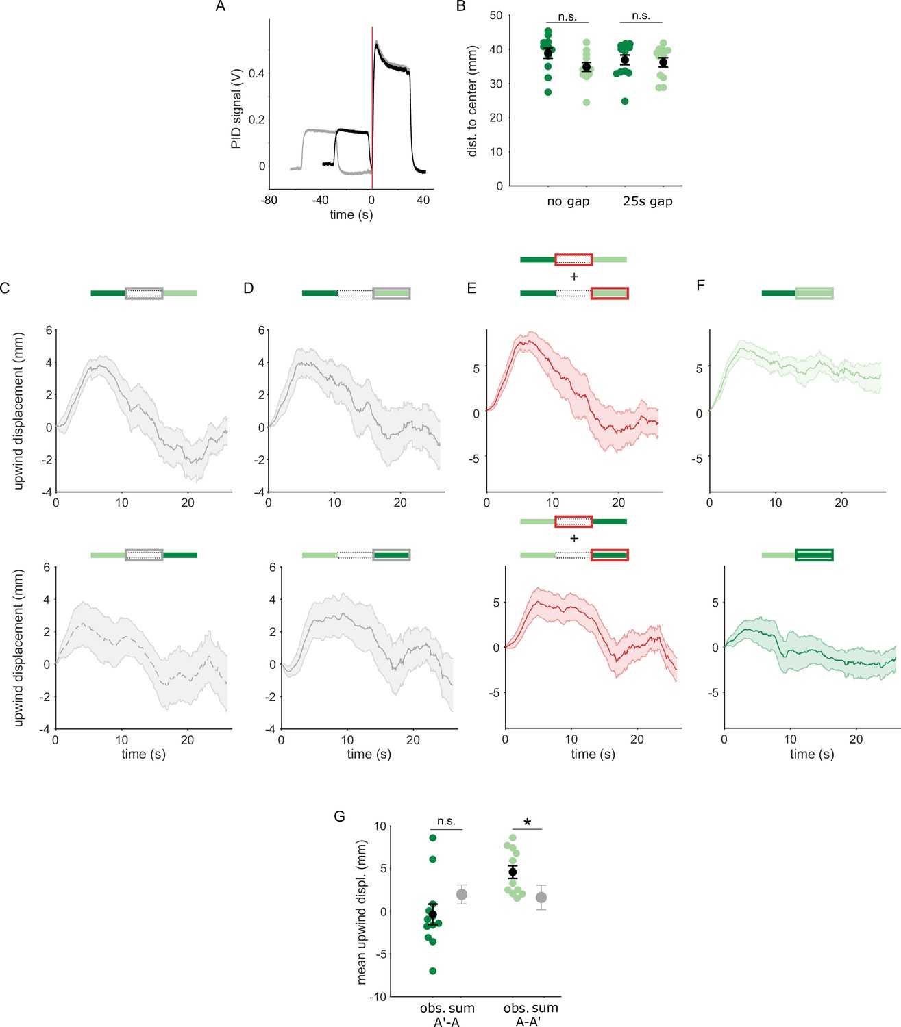
Transition dependent attraction is not a result of linearly summed, single-pulse responses.
(A) PID measurements of odor time courses in the behavioral arena, measured at the central exhaust port. The black trace depicts odor pulses delivered with no gap and the gray trace depicts pulses interrupted by a 25 s air period. The vertical red line indicates the time point identified as the onset of the second odor pulse. (B) Mean distances of flies from the arena center at the onset of the second odor pulse in each experiment. Distances from the center were not significantly different between experiments with the unpaired and paired odor, with a 0 s gap (n=12, 12 resp. p=0.08) or with a 25 s gap (n=12, 13, p=0.39). Statistical comparisons made with the independent samples, Wilcoxon’s rank sum test followed by a Bonferroni-Holm correction for multiple comparisons. (C) The off response trace after the first odor pulse for A-A’ transitions without an air gap (top) and A’-A transitions with an air gap (bottom). (D) The response at the onset of the second odor pulse for A-A’ transitions without an air-gap (top) and A’-A transitions with an air gap (bottom). (E) The linear sum of upwind displacement traces in C and D. This is the null model to compare with responses to an odor transition. (F) Actual displacement during the second odor pulse in unpaired to paired transition stimuli with no air-gap. Traces in C–F are mean +/-SEM. (G) Mean upwind displacement over the duration of the second odor pulse for the two transitions (dark green: A’ to A, light green; A to A’). In gray is the mean and bootstrapped SEM of the linear sum of component responses in C. The measured displacements are significantly greater than the sum when odor A’ is second (n=12, p=0.001) but not when odor A is second (n=12, p=0.09). Displacements were compared with the Wilcoxon’s signed rank test followed by a Bonferroni-Holm correction for multiple comparisons.
Figure 6—figure supplement 2
Flies reinforced via DAN PPL1-α3 do not respond to transitions between A and A’.
Flies were trained by pairing one of the similar odors with optogenetic activation of DAN PPL1-α3. They were then tested with 30 s odor pulses presented either as direct transitions (A,B) or interrupted by a 25 s air period (C,D), as in Figure 6. Transition order indicated by the bars on top of panels A-D. (A) Upwind displacement in the first and second pulses of an A-A’ odor transition. Traces in dark and light green are responses to A and A’ respectively. Plots are mean +/-SEM (n=8 arena runs for all stimulus types). (B) Upwind displacement for the reverse odor transition i.e. A’-A. (C) Upwind displacement for A-gap-A’ interrupted transition. (D) Upwind displacement for the reversed, A’-gap-A interrupted transition. (E) Upwind displacement in response to the first odor pulse, averaged across flies in each arena experiment. Mean displacement was not significantly different between unpaired and paired odors for experiments with no gap (n=8 experiments each for paired and unpaired odors, p=0.28) and a 25 s gap (n=8, p=0.69). (F) As in E except for responses to the second odor pulse. Unlike with DAN PPL1-γ2α’1, displacement was not significantly different for transitions with no gap between pulses (n=8, p=0.78) or when transitions were interrupted by a 25 s gap (n=8, p=0.57). Statistical comparisons in E and F were made with the independent-sample Wilcoxon rank sum test with a Bonferroni-Holm correction for multiple comparisons.
Additional files
Download links
A two-part list of links to download the article, or parts of the article, in various formats.
Downloads (link to download the article as PDF)
Open citations (links to open the citations from this article in various online reference manager services)
Cite this article (links to download the citations from this article in formats compatible with various reference manager tools)
Flexible specificity of memory in Drosophila depends on a comparison between choices
eLife 12:e80923.
https://doi.org/10.7554/eLife.80923


