Patterns of interdivision time correlations reveal hidden cell cycle factors
Figures
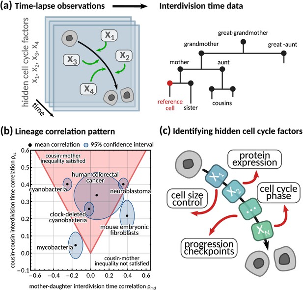
Using interdivision time data on lineage trees to infer the hidden cell cycle factors.
(a) Time lapse observations. Cartoon demonstrating how time-lapse microscopy allows single cells to be tracked temporally as they go through the cell cycle to division. Multiple different factors affect the rate at which cells progress through the cell cycle from birth to subsequent division. Interdivision time data. Example lineage tree structure with possible ‘family relations’ of a cell between which correlations in interdivision time can be calculated. (b) Lineage correlation pattern. Plot of mother-daughter interdivision time correlation against cousin-cousin interdivision time correlation for the six publicly available datasets used in this work (Appendix 1—table 1, Martins et al., 2018; Priestman et al., 2017; Chakrabarti et al., 2018; Kuchen et al., 2020; Mura et al., 2019). The shaded red area indicates the region where the cousin-mother inequality is satisfied. (c) Identifying hidden cell cycle factors. Schematic showing the model motivation and process. We produce a generative model that describes the inheritance of multiple hidden ‘cell cycle factors’ that affect the interdivision time. The model is fitted to lineage tree data of interdivision time, and we analyse the model output to reveal the possible biological factors that affect the interdivision time correlation patterns of cells.
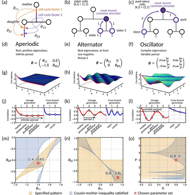
Analysis of the inheritance matrix model identifies three distinct lineage tree correlation patterns.
(a) Diagram illustrating the inheritance matrix model with two cell cycle factors which affect the interdivision time of a cell. Each factor in the mother exerts an influence on a factor in the daughter through the inheritance matrix . (b,c) Schematics showing how the coordinate introduced in ‘The inheritance matrix model reveals three distinct interdivision time correlation patterns’ is determined. This coordinate describes the distance to the most recent common ancestor for chosen pair of cells. Examples shown are (b) sister pairs with , and (c), aunt-niece pairs with . (d-o) Panels demonstrating the three correlation patterns that arise from the inheritance matrix model with two cell cycle factors. (d-f) Example inheritance matrices that produce the desired patterns: (d) aperiodic, (e) alternator and (f) oscillator correlation patterns. (g–i) Three-dimensional plot of the generalised tree correlation function (Equation M3) demonstrating each of the three patterns. On each plot we highlight the lineage generation correlation function ( or ) (red line) and the cross-branch generation correlation function () (blue line). The shading of the 3D plot indicates the correlation coefficient at that point on the surface. (j–l) The lineage and cross-branch generation correlation functions plotted individually, showing the different dynamics for each pattern. (m–o) Region plots showing parameter values where the relevant pattern is obtained (orange) and where the cousin-mother inequality is satisfied (blue) for the matrices given in panels (d-f). White bands on (o) indicate where which results in real eigenvalues and therefore does not produce an oscillator pattern. Within the parameter region that both produces the desired pattern and also satisfied the cousin-mother inequality, we choose a parameter set (red cross) which is used for the corresponding plots in the panels above. In all panels we fix and the noise vector to have covariance equal to the identity matrix.
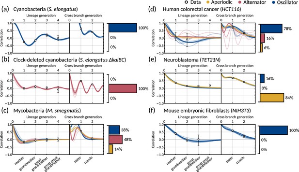
The inheritance matrix model with two cell cycle factors fits interdivision time correlation patterns for a range of cell types.
Posterior correlation functions based on fitting to mother-daughter, grandmother-granddaughter, sister-sister and cousin-cousin correlations for three bacterial (left) and three mammalian (right) datasets: (a) cyanobacteria, (b) clock-deleted cyanobacteria, (c) mycobacteria, (d) human colorectal cancer, (e) neuroblastoma, and (f) mouse embryonic fibroblasts. Pearson correlation coefficients (white circles) and 95% bootstrapped confidence intervals (error bars) obtained through re-sampling with replacement of the original data (10,000 re-samples). Posterior distribution samples were clustered into aperiodic, alternator, and oscillator patterns (bar charts). We show multiple representative samples (solid and shaded lines) drawn from the posterior distribution Appendix 1—figure 2 without clustering. Where correlations appear missing, this is in cases where the lineage trees in the data were not deep enough for the correlations to be calculated. Only lineage and cross branch generations 1 and 2 were used in model fitting. Here all panels assume , but taking produces similar results (Appendix 1—figure 4).
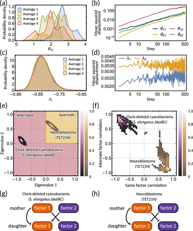
Bayesian inference predicts hidden dynamical correlations between cell cycle factors.
(a) Posterior distribution histograms for depend on the realisations of a Gibbs sampler and do not settle to a stationary distribution. (b) A log-log plot of mean squared displacement for the four variables that make up the inheritance matrix . The mean squared displacement for all four parameters increases linearly, meaning the sampling does not settle in any particular region of parameter space. (c) Sampled posterior distribution histograms for the eigenvalue for each realisation. The histograms are almost identical across the four averages, showing the distribution has converged. (d) Mean squared displacement for the eigenvalues of the inheritance matrix settles to a finite value. Plots (a) - (d) utilise sampling from the inference for the clock-deleted cyanobacteria dataset. (e) Density histogram of the real eigenvalue pairs for clock-deleted cyanobacteria (pink) and neuroblastoma (brown) demonstrating where the eigenvalues lie in the aperiodic (yellow) and alternator (red) regions. (f) Density histogram of same-factor against alternate-factor mother-daughter correlation for clock-deleted cyanobacteria (pink) and neuroblastoma (brown). We take a minimum threshold of 0.3 for the probability density to remove irrelevant samples. (g–h) Influence diagrams for same factor vs alternate factor correlations for (g) clock-deleted cyanobacteria and (h) neuroblastoma.
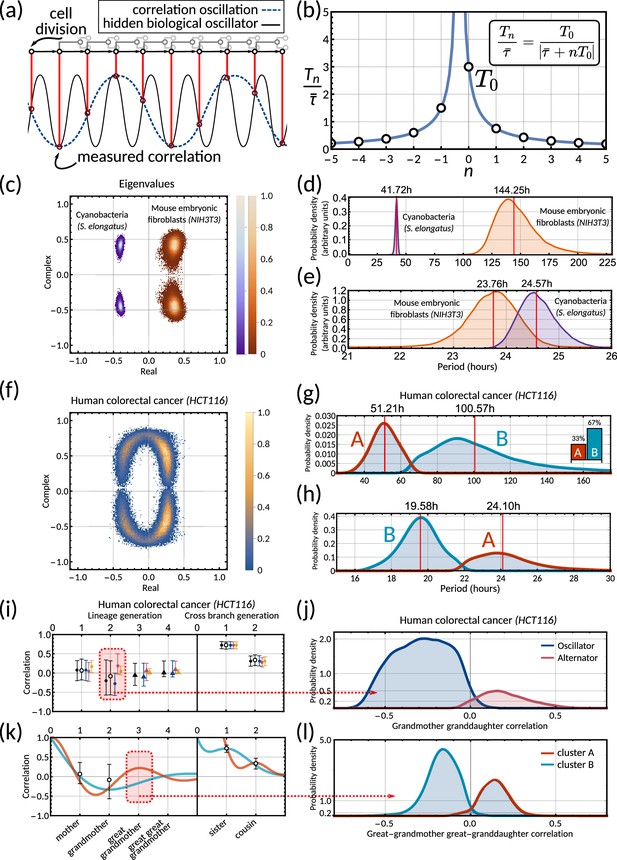
The inheritance matrix reveals the periodicity of hidden biological oscillators underlying the cell cycle.
(a) Schematic showing how sampling a high frequency rhythm at each cell division could result in a lower frequency oscillator being constructed. (b) Possible oscillator periods (Equation 7) indexed by for a correlation oscillation period . (c) Density plot of the complex eigenvalue output from the model sampling for cyanobacteria (purple) and mouse embryonic fibroblasts (orange). (d) Posterior distributions of the correlation oscillation period in cyanobacteria (purple) and mouse embryonic fibroblasts (orange). (e) Posterior distributions of the oscillator period in cyanobacteria (purple) and mouse embryonic fibroblasts (orange). Arbitrary units in (d) and (e) are used to compare histograms, the density values are not normalised in relation to each other in order to display both histograms clearly on the same plot. (f) Density plot of complex eigenvalues for human colorectal cancer. (g) Posterior distributions of the correlation oscillation period in human colorectal cancer (shaded area) and oscillator clusters corresponding to positive (cluster A, orange) and negative real parts (cluster B, blue). The bar chart shows the posterior mass of the clusters. (h) Posterior distributions of the oscillator periods corresponding to (g). (i) Model fit and 95% credible intervals for human colorectal cancer (cf. legend of Figure 3). Red area indicates the grandmother granddaughter correlation explored in (j). (j) Posterior distribution of oscillator vs alternator clusters give grandmother correlations with opposite signs. (k) Lineage and cross-branch correlation functions of oscillator clusters A (orange) and B (blue) in human colorectal cancer. Red area indicates the great-grandmother great-granddaughter correlation explored in (l). (l) Posterior distributions of oscillator clusters A (orange) and B (blue) have great-grandmother correlations of opposite signs.
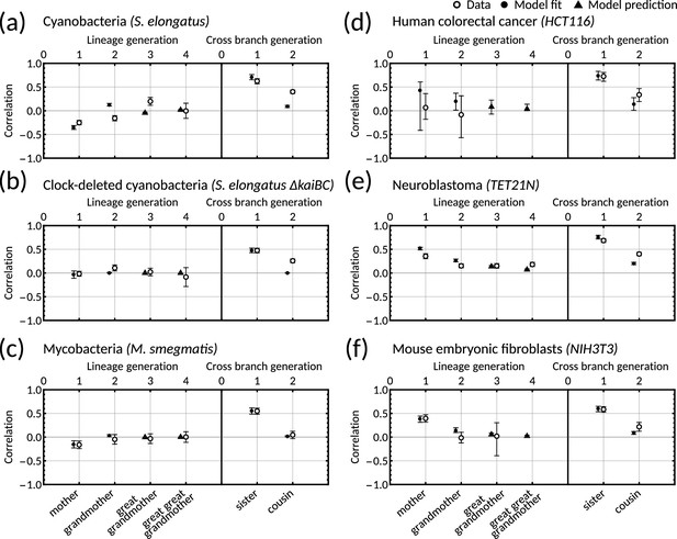
One-dimensional model with simple inheritance rules results in a poor fit for datasets displaying the cousin-mother inequality.
(a–f) Plots showing data (open markers) against model predictions (solid black) for the one-dimensional model Cowan and Staudte, 1986 for (a) cyanobacteria, (b) clock-deleted cyanobacteria, (c) mycobacteria, (d) human colorectal cancer, (e) neuroblastoma and (f) mouse embryonic fibroblasts. We fit the model using the same likelihood function (Equation M10) and methods (Materials and methods - ‘Data analysis and Bayesian inference of the inheritance matrix model‘) as in the main text. Points (black) give the median model output for each correlation and error bars give the 95% bootstrapped confidence intervals from 10,000 re-samplings with replacement. Circular points show the model fitted correlations (mother-daughter, grandmother-granddaughter, sister-sister and cousin-cousin) whereas triangular points demonstrate model predictions. For this fitting we used 100,000 samples (in contrast to 10 million used in the main text).
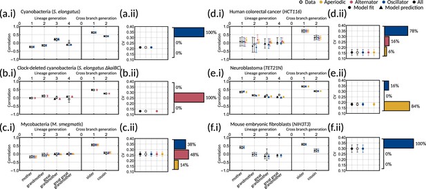
Bayesian inference demonstrates that multiple correlation patterns can explain the experimental data.
(a-f.i) Plots of model fits and predictions (solid markers) against the data (open markers) for the family pair correlation coefficients for (a) cyanobacteria, (b) clock-deleted cyanobacteria, (c) mycobacteria, (d) human colorectal cancer, (e) neuroblastoma and (f) mouse embryonic fibroblasts. Colours of the solid markers represent the fits and predictions for parameter samples clustered by correlation pattern. Inset for each panel is a bar chart giving the distribution of the three patterns for each dataset. (a-f.ii) Plots of model output against the data for the interdivision time covariance. In this figure, the error bars for the data (unfilled black points) are calculated via bootstrapping of 10,000 samples with replacement to give the 95% confidence interval. For the model, error bars represent the 95% credible interval, computed by taking the 2.5th and 97.5th percentile of the sampled values. For all plots, circles indicate fitted correlations and triangles show predicted correlations. We can see that the model fit is good for all datasets as the error bars overlap with that of the data, and this is reflected in the low AIC given in Appendix 1—table 1.

The log-likelihood converges during the parameter inference.
(a) Trace of the log-likelihood from four initialisations of the inference on the clock-deleted cyanobacteria dataset (different colours). (b) Histogram of the posterior distribution of the log-likelihood for the inference samples on the clock-deleted cyanobacteria dataset. The histogram for each average aligns demonstrating convergence of the log-likelihood.
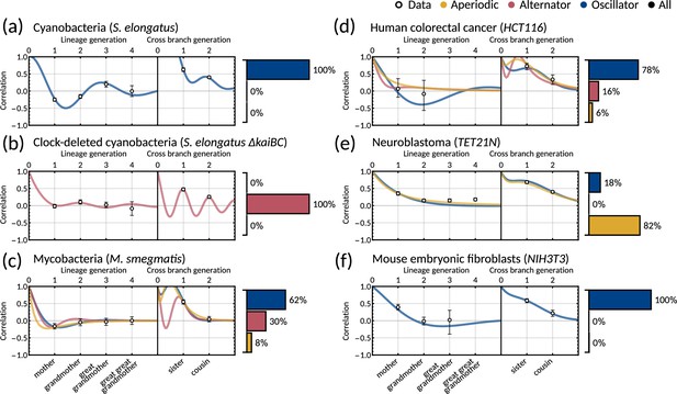
Two-dimensional inheritance matrix model gives a good fit for
Same panels as in Figure 3 but with and showing only one sample. We show the calculated family correlations with 95% bootstrapped confidence intervals (open markers) and a single sample of the model fit for (a) cyanobacteria, (b) clock-deleted cyanobacteria, (c) mycobacteria, (d) human colorectal cancer, (e) neuroblastoma and (f). Posterior parameter sets are clustered by correlation patterns (bar charts.) For this fitting we used 100,000 samples (in contrast to 10 million used in the main text). We see a similar fit and pattern distributions for all cell types except for mycobacteria (c), which here displays a dominant oscillator pattern.
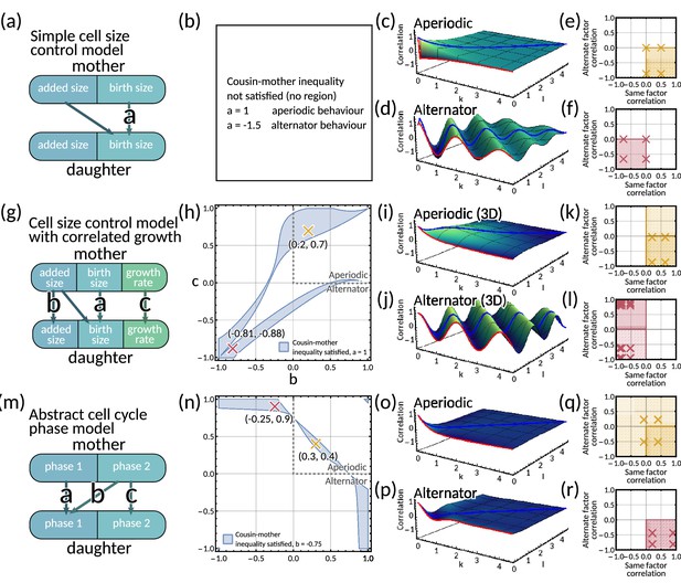
Mapping mechanistic models to the inheritance matrix model framework.
(a–f) Simple cell size control model. (a) Model schematic. (b) The cousin-mother inequality cannot be satisfied for any choice of parameter . (c–d) Generalised tree correlation function plots (c) for and (d) resulting in aperiodic and an alternator pattern respectively. (e–f) Same vs alternate factor mother-daughter correlation plots for (e) and (f). In panels (b–f) we fix . (g–l) Cell size control model with correlated growth rate. (g) Model schematic. (h) Region plot with fixed parameter showing the parameter space that satisfies the cousin-mother inequality (blue). Example parameter choices are also plotted for an aperiodic (yellow) and an alternator (red) pattern. (i–j) Generalised tree correlation function plots for (i) and (j) resulting in aperiodic and an alternator pattern respectively. (k,l) Same vs alternate factor mother-daughter correlation plots for (k) and (l). In panels (h–l) we fix . (m–r) Two cell cycle phase model (m) Model schematic. (n) Region plot with fixed parameter showing the parameter space that satisfies the cousin-mother inequality (blue). Example parameter choices are also plotted for an aperiodic (yellow) and an alternator (red) pattern. (o–p) Generalised tree correlation function plots (o) for and (p) resulting in aperiodic and an alternator pattern respectively. (q–r) Same vs alternate factor mother-daughter correlation plots for (q) and (r). In panels (n–r) we fix .
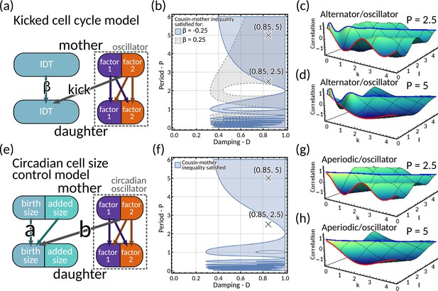
Models of circadian-clock-driven correlation patterns (a–d) Kicked cell cycle model.
(a) Model schematic. The mother to daughter IDT inheritance is given by where is the size control parameter. The ‘kick’ to the cell cycle us produced by a two-dimensional complex eigenvalued inheritance matrix model system with oscillator behaviour. (b) Region plot for (blue) and (grey), demonstrating the region for this model where the cousin inequality is satisfied. Here we fix the variances of the noise terms and all equal to 0.1. (c–d) Plot of the generalised tree correlation function for (c) and (d) . In both these plots we take , meaning the model has a mixture of alternator and oscillator behaviours. The cousin inequality is satisfied for both these parameter choices. (e–h) Circadian cell size control model (e) Model schematic. The parameter gives how the daughter’s birth size depends on the mother’s birth size; and gives the coupling of the circadian oscillator to the size control. (f) Region plot demonstrating where the cousin inequality is satisfied. We fix . Correlations between noise terms are fixed equal to 0 and we set for . (g–h) Plots of the generalised tree correlation function for the same fixed parameters specified in panel (f), with (g) , and (h) . As we fix , these plots show a combination of aperiodic and oscillator behaviour. We note that for , the cousin inequality is not satisfied. This demonstrate that oscillatory behaviour is not a necessary condition for the cousin inequality to be satisfied.
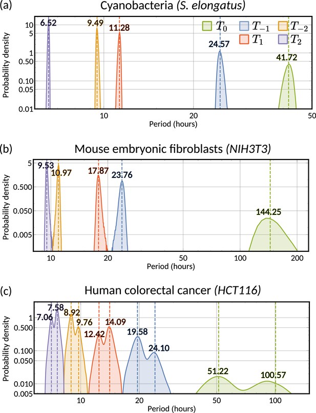
A range of oscillator periods can explain oscillatory interdivision time patterns.
Histogram of the posteriors of the possible periods underlying the lineage correlation function for (a) cyanobacteria, (b) mouse embryonic fibroblasts and (c) human colorectal cancer, calculated using Equation 7. Numerical values give medians of the posterior distributions for each . For (c) human colorectal cancer, we take the median period of each cluster where the clusters are allocated through the sign of the real part of the eigenvalue (see Figure 5f). For all panels the correlation oscillation period is given in green and the oscillator periods in different colours. The period analysed in ‘The inheritance matrix model predicts the hidden dynamical correlations of cell cycle factors’ corresponds to the histograms of (blue).
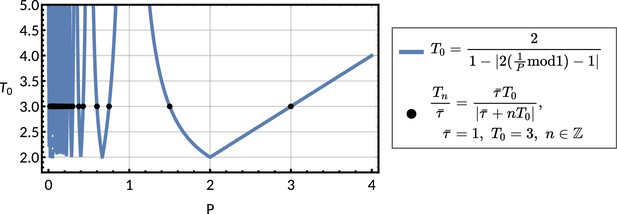
Observed period against chosen period parameter for a forced oscillator pattern.
Plot of the function for against the observed lineage correlation function period given in Equation M9 (blue line), for an oscillator pattern given in ‘The inheritance matrix model reveals three distinct interdivision time correlation patterns’. We see that for . For chosen with and various we see how the parameters that produce the corresponding s are directly equal to the possible we can derive from the chosen (black points), using Equation 7.
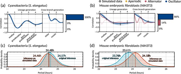
Validation of the Bayesian inference method using simulated data.
Model fits and distribution of patterns for data simulated using the maximum posterior parameter set (Appendix 1—table 2) for (a) cyanobacteria, and (b) mouse embryonic fibroblasts. To simulate interdivision time lineage trees, we take the maximum posterior parameter sets from the original inference on the two datasets. These trees are simulated using Equation 2a in MATLAB using custom scripts which utilise ‘Random trees’ branching process (Kaj and Gaigalas, 2022). For each dataset, we first simulate a complete tree of 11 generations (2047 cells) and take the last 1000 cells to sample stationary initial conditions. For the final simulated data, we simulated a number of smaller trees of 6 generations (63 cells each) to better represent live imaging experiments. We divide the number of cells in the original dataset by 63 and simulate this number of trees, with each tree having initial condition sampled from the last 1000 cells of the original large tree. We then randomly sample 85% of the simulated cells without replacement to imitate loss of cells from imaging mid experiment. The calculation of the family interdivision time correlation coefficients and the parameter inference was done in the same way as with the original datasets as outlined in Materials and methods - ‘Data analysis and Bayesian inference of theinheritance matrix model’. Pearson correlation coefficients (white dots) and 95% bootstrapped confidence intervals (error bars) were obtained through re-sampling with replacement (10,000 samples) of the simulated data. Posterior samples were clustered into aperiodic, alternator, and oscillator patterns (bar charts). We show several representative samples (solid and shaded lines) of the model fit drawn from the posterior distribution. We assume . (c–d) Histograms of the inferred oscillator period for the original inference (blue) and inference on the simulated data (orange) for cyanobacteria (c) and mouse embryonic fibroblasts (d), demonstrating significant overlap of the oscillator period of the simulated parameter set (black dashed line) and the posterior distribution from Bayesian inference. Note that the posterior distributions of the real (red) and simulated datasets (blue) also overlap. Dashed lines give the median period of these posterior distributions for original inference (blue) and inference on simulated data (orange). Maximum posterior parameters used in the simulations are given in Appendix 1—table 2.
Tables
Lineage tree statistics obtained from each dataset used in this work.
Mean interdivision time, tree variance, CVs and all correlation coefficients ± standard deviation of the bootstrap distributions from 10,000 re-samplings with replacement. Statistics were calculated on all available cells that could be put in the required family pair (Materials and methods - ‘Data analysis and Bayesian inference of the inheritance matrix model’). Shaded datasets exhibit the cousin-mother inequality.
| Cell type | Mean (hours) | Variance (hours2) | CV | 1D AiC | 2D AiC | ref. | ||||
|---|---|---|---|---|---|---|---|---|---|---|
| Cyanobacteria (S. elongatus) | 15.47±3.27 | 10.67±0.36 | 0.21±0.004 | −0.25±0.024 | −0.16±0.028 | 0.63±0.028 | 0.40±0.019 | 408.13 | 14.01 | Martins et al., 2018 |
| Clock deleted cyanobacteria (S. elongatus ΔkaiBC) | 14.43±1.89 | 3.57±0.15 | 0.13±0.003 | −0.02±0.027 | 0.12±0.032 | 0.48±0.025 | 0.26±0.021 | 172.47 | 14.00 | Martins et al., 2018 |
| Mycobacteria (M. smegmatis) | 2.52±0.65 | 0.42±0.03 | 0.26±0.010 | −0.16±0.041 | −0.05±0.051 | 0.55±0.033 | 0.05±0.040 | 8.69 | 14.01 | Priestman et al., 2017 |
| Human colorectal cancer (HCT116) | 16.39±2.55 | 6.49±1.10 | 0.15±0.012 | 0.07±0.141 | −0.08±0.227 | 0.73±0.047 | 0.34±0.070 | 22.20 | 14.23 | Chakrabarti et al., 2018 |
| Neuroblastoma (TET21N) | 17.12±3.13 | 9.79±0.68 | 0.18±0.006 | 0.35±0.027 | 0.15±0.022 | 0.69±0.021 | 0.40±0.018 | 196.79 | 14.00 | Kuchen et al., 2020 |
| Mouse embryonic fibroblasts (NIH3T3) | 20.40±6.09 | 37.03±4.31 | 0.30±0.015 | 0.39±0.040 | −0.01±0.057 | 0.59±0.029 | 0.22±0.047 | 21.64 | 14.01 | Mura et al., 2019 |
Maximum posterior matrices from the original inference, used to simulate interdivision time trees used for analysis in Appendix 1 - Section A8 Appendix 1—figure 9.
| Matrix | Cyanobacteria(S.elongatus) | Mouse embryonicfibroblasts (NIH3T3) |
|---|---|---|
Comparison of different variance estimators.
Mean and 95% confidence intervals calculated from bootstrap distributions of 10,000 re-samplings with replacement for each dataset used in this work. The estimators are obtained as follows: bare variance is computed using all available cells that could be put in the required family pair (Materials and methods - ‘Data analysis and Bayesian inference of theinheritance matrix model’). The lineage variance is calculated through the weighted variance with weights following arguments similar to Priestman et al., 2017; Nozoe et al., 2017. Here is the number of divisions in the lineage that came before cell and is the total number of trees in the whole dataset. The censored variance is calculated after pruning trees such that each tree contains lineages of the same length as in Kuchen et al., 2020; Sandler et al., 2015.
| Cell type | Bare variance (hours2) | Lineage variance (hours2) | Censored variance (hours2) |
|---|---|---|---|
| Cyanobacteria (S. elongatus) | 10.674 [9.966, 11.396] | 11.543 [10.420, 12.776] | 10.612 [9.850, 11.391] |
| Clock deleted cyanobacteria (S. elongatus ∆kaiBC ) | 3.573 [3.288, 3.865] | 4.015 [3.529, 4.512] | 3.485 [3.176, 3.805] |
| Mycobacteria (M. smegmatis) | 0.427 [0.366, 0.494] | 0.601 [0.490, 0.716] | 0.609 [0.492, 0.738] |
| Human colorectal cancer (HCT116) | 6.489 [4.540, 8.809] | 7.357 [4.898, 10.262] | 6.741 [4.695, 9.124] |
| Neuroblastoma (TET21N) | 9.794 [8.539, 11.213] | 13.986 [10.735, 17.775] | 10.502 [8.554, 12.621] |
| Mouse embryonic fibroblasts (NIH3T3) | 37.032 [29.260, 46.162] | 46.378 [34.494, 60.090] | 39.418 [29.947, 50.219] |


