Translational rapid ultraviolet-excited sectioning tomography for whole-organ multicolor imaging with real-time molecular staining
- Translational and Advanced Bioimaging Laboratory, Department of Chemical and Biological Engineering, The Hong Kong University of Science and Technology, China
Figures
Figure 1 with 9 supplements
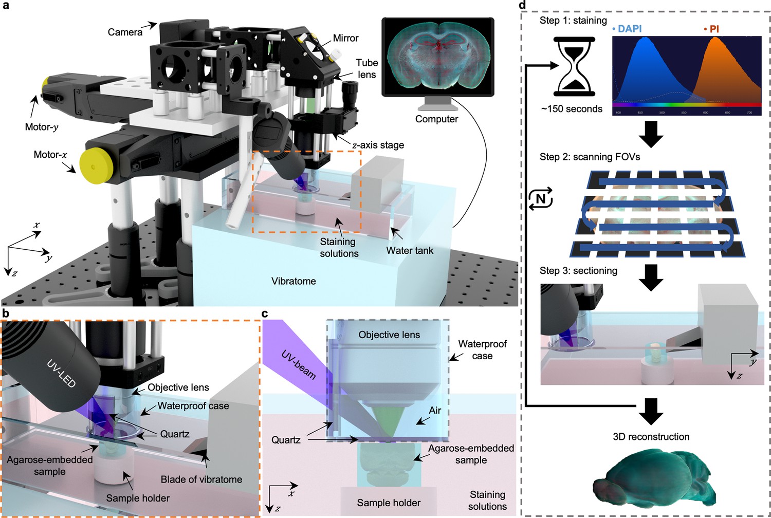
Overview of 3D whole-organ imaging by TRUST.
(a) Schematic of the TRUST system. Light from UV-LED is obliquely projected onto the surface of an agarose-/gelatin-embedded sample (e.g., a mouse brain), which is placed on top of a sample holder inside a water tank of a vibratome filled with staining solutions. The generated fluorescence and autofluorescence signals are collected by an objective lens, refocused by an infinitely corrected tube lens, and finally detected by a color complementary metal-oxide-semiconductor camera. (b), Close-up of the region marked by orange dashed box in a, showing the components immersed in the staining solutions. (c), Viewing b from the x-z plane. A waterproof case containing two pieces of quartz keeps most of the space under the objective lens filled with air. (d), Workflow of the whole imaging process, including (1) chemical staining for ~150 s, (2) widefield imaging with raster-scanning and stitching in parallel, and (3) shaving off the imaged layer with the vibratome to expose a layer underneath. The three steps will be repeated until the entire organ has been imaged. All procedures are automated with lab-built hardware and control programs.
Figure 1—figure supplement 1
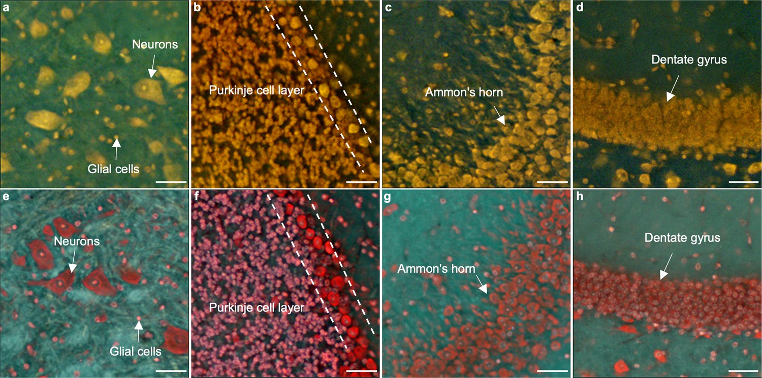
Comparison of single labeling (PI) and double labeling (DAPI and PI).
(a–d) TRUST images of a fixed mouse brain stained by PI. (e–h) TRUST images of similar regions from another mouse brain stained by DAPI and PI. White arrows and dashed lines indicate several typical structures of the brain, such as the Purkinje cell layer or dentate gyrus. Scale bars: 50 µm.
Figure 1—figure supplement 2
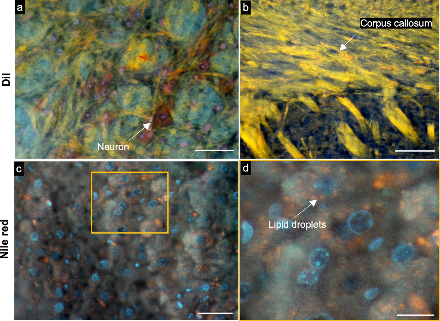
TRUST images of brain and liver tissues stained with Dil and Nile red.
(a), TRUST image acquired with a 10× / 0.3 NA objective lens of mouse brain tissue which is simultaneously stained by DAPI, PI, and Dil with the concentration of 5 µg/ml. (b) TRUST image acquired with a 10× / 0.3 NA objective lens of mouse brain tissue which is stained with Dil only. (c) TRUST image acquired with a 20× / 0.4 NA objective lens of mouse liver tissue which is stained with both DAPI and Nile red with the concentration of 5 µg/ml. (d), Close-up image of the yellow solid region marked in c. Scale bars: 50 µm (a,c), 100 µm (b), and 20 µm (d).
Figure 1—figure supplement 3

The schematic of the customized 2-axis adjustable angular platform under the vibratome.
A hemispherical steel body serves as the fulcrum and four adjustable screws allow pitching and rolling adjustment of the aluminum supporting plate.
Figure 1—figure supplement 4
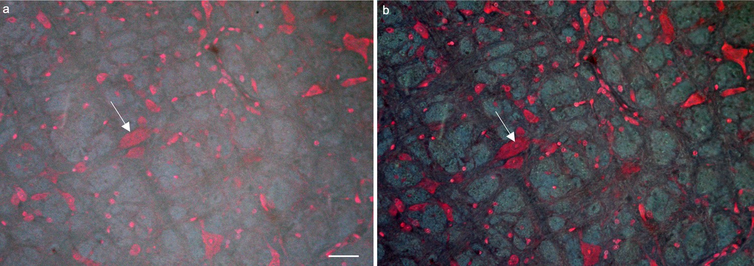
High imaging contrast enabled by a waterproof case.
(a) TRUST image of a mouse brain without installing a waterproof case. (b) TRUST image of the same region in a with a waterproof case. The image contrast of b (e.g., the cell marked by the white arrow) is better than that of a. Scale bars: 50 µm.
Figure 1—figure supplement 5
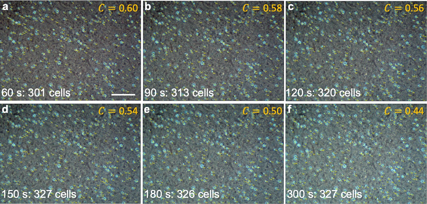
Estimation of staining time by cell counting.
(a–f) Cell counting of the same region in fixed liver tissue at 60 s, 90 s, 120 s, 150 s, 180 s, and 300 s, after the tissue layer has been exposed to the staining solutions (DAPI: 5 µg/ml). The staining time is estimated to be ~150 s, as the number of cells is almost the same after this time point. The image contrast is provided for each time point. Scale bar: 100 µm (a–f).
Figure 1—figure supplement 6
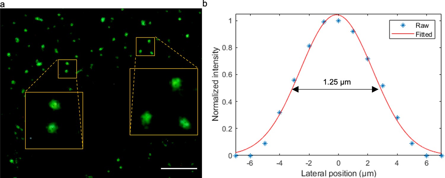
Experimental characterization of TRUST’s lateral resolution.
(a) Imaging results of green-fluorescent beads (G200, Thermo Fisher Scientific Inc) with an average diameter of 0.2 µm. (b) Averaged spatial light intensity distributions of 10 beads in a were plotted with blue asterisks, and the corresponding Gaussian fitted curve was plotted with a solid red line. Defined by the full-width at half maximum of the fitted curve, the lateral resolution of the TRUST system with a 10× / 0.25 NA objective lens is ~1.25 µm. Scale bar: 20 µm.
Figure 1—figure supplement 7
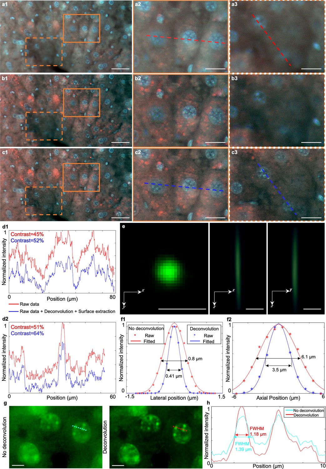
Image quality comparison of TRUST images with deconvolution and surface extraction.
(a1), Single frame from a z stack images acquired by TRUST with a 20× / 0.4 NA objective lens at an interval of 2 µm. (a2), (a3) Two close-up images of the solid and dashed regions marked in a1, respectively. (b1), Reconstructed image of a1 with 10 iterations of a Lucy–Richardson algorithm Dey et al., 2006 conducted by an open-source ImageJ Schneider et al., 2012 plugin, DeconvolutionLab2 Sage et al., 2017. (b2), (b3) Two close-up images of the solid and dashed regions marked in b1, respectively. (c1), Reconstructed image of b1 after applying focal stacking to extend the depth-of-field performed by another ImageJ plugin based on a complex wavelet approach Forster et al., 2004. (c2), (c3) Two close-up images of the solid and dashed regions marked in c1, respectively. (d1), Intensity profiles of the red dashed and blue dashed lines from a2 and c2. (d2), Intensity profiles of the red dashed and blue dashed lines from a3 and c3. (e) Orthogonal and cross-sectional views of the point spread function of the TRUST system with a 20× / 0.4 NA objective lens measured with green-fluorescent beads with an average diameter of 0.2 µm. The scanning step size along the axial direction is 1 µm. (f1), Comparison of the lateral resolution of the TRUST system with/without deconvolution which is defined by the full width at half maximum of the fitted curve. (f2), Comparison of the axial resolution of the TRUST system with/without deconvolution. Near two times resolution improvement has been obtained in both lateral and axial directions. (g) Two zoomed-in regions from the green channel of TRUST images for mouse kidney tissue stained by 5 µg/ml DAPI show that deconvolution enables resolution and contrast to be improved. (h), Line profiles of cyan and red dashed lines region marked in g show that the FWHM of the nuclei is smaller (more resolved) with deconvolution than without. Scale bars: 50 µm (a1,b1,c1), 20 µm (a2,a3,b2,b3,c2,c3), 2 µm (e), and 5 µm (g).
Figure 1—figure supplement 8
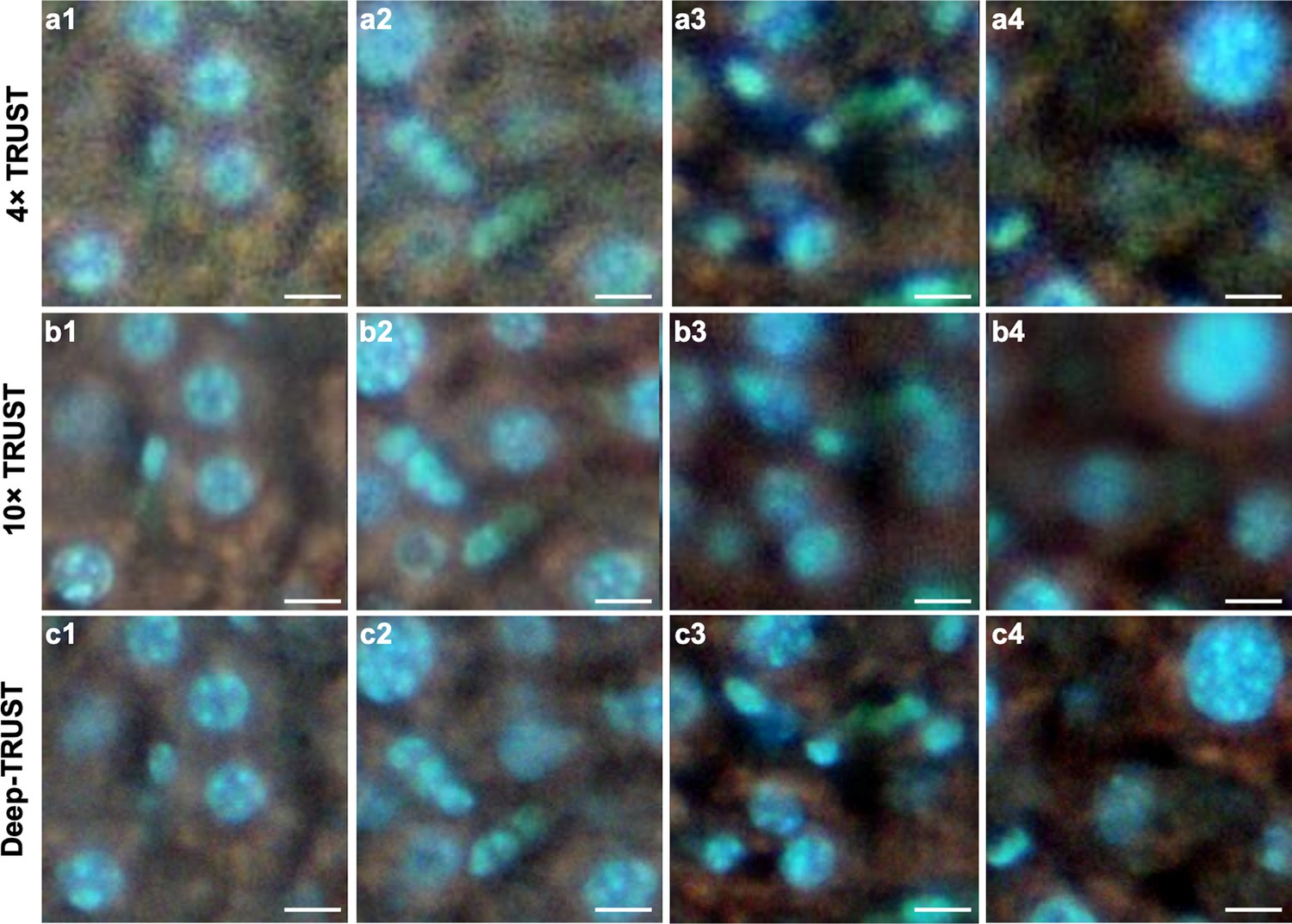
Comparison of imaging results from 4×TRUST, 10×TRUST, and Deep-TRUST.
(a1–a4) TRUST images acquired with a 4× / 0.1 NA objective lens. (b1–b4) TRUST images acquired with a 10× / 0.3 NA objective lens. (c1–c4) Output images from the ESRGAN Wang, 2019 neural network trained with another group of paired 4×and 10×TRUST images. Scale bars: 10 µm.
Figure 1—video 1
Recycling of sectioned slices with a pump.
Figure 2 with 7 supplements
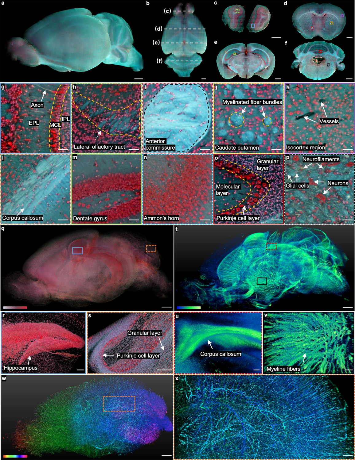
Whole mouse brain imaging with TRUST.
(a, b), Side and top views of the reconstructed 3D model of a fixed mouse brain, respectively. (c–f) Four coronal sections with positions indicated in b by the white dashed lines. (g), (h), Close-up images of the blue solid and green dashed regions marked in c. (i–k), Close-up images of the red dotted, yellow dashed, and purple solid regions marked in d. (l–n), Close-up images of the orange dotted, green solid, and blue dashed regions marked in e.( o), (p), Close-up images of the red solid and black dashed regions marked in f. (q), The cell nuclei in the mouse brain extracted from the red channel in a. (r), ( s), Close-up images of the blue solid and orange dashed regions marked in q. (t), 3D structure of the nerve tracts or fibers extracted from the green channel of the autofluorescence signal in a. (u), (v), Close-up images of the red dashed and black solid regions marked in t. (w), Vessel network extracted from another mouse brain and rendered with different colors corresponding to different coronal layers. (x), Close-up image of the orange dashed region marked in w. MCL: mitral cell layer; IPL: inner plexiform layer; EPL: external plexiform layer. Scale bars: 1 mm (a–f, q,t,w), 200 µm (x), 100 µm (r–v), and 50 µm (g–p).
Figure 2—figure supplement 1
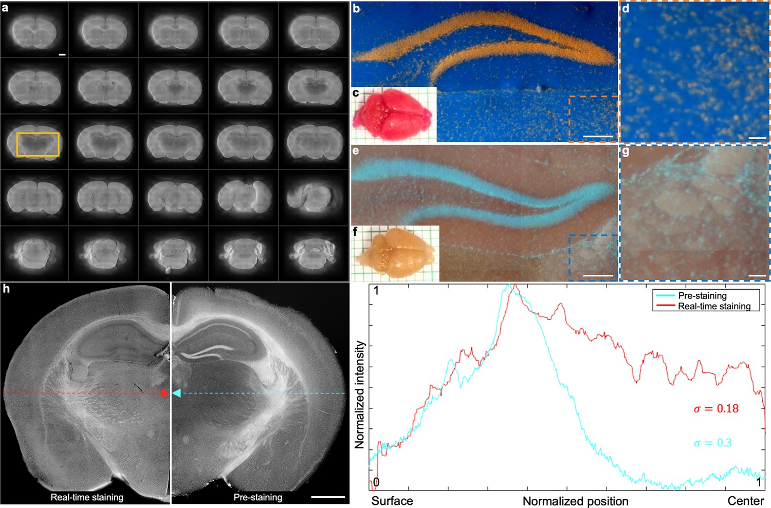
Potential side effects of conventional chemical staining protocol Seiriki et al., 2019.
(a) Multiple grayscale sections of the brain in f which show that the inner areas in the brain (marked with the yellow solid box) appear to be darker than the peripheral areas due to the nature of passive diffusion. (b) Hippocampus region of the brain in c which has been fully stained by PI. (d) A close-up image of the orange dashed region marked in b. (e) Hippocampus region of the brain in f which has been fully stained by Hoechst 33342 and rhodamine. (g) A close-up image of the blue dashed region marked in e. (h), Normalized intensity distribution profiles of the brain section with real-time staining (left half and marked with dashed red arrow) and pre-staining (right half and marked with dashed cyan arrow). Scale bars: 1 mm (a), 500 µm (b,e), 100 µm (d,g), and 1 mm (h).
Figure 2—figure supplement 2
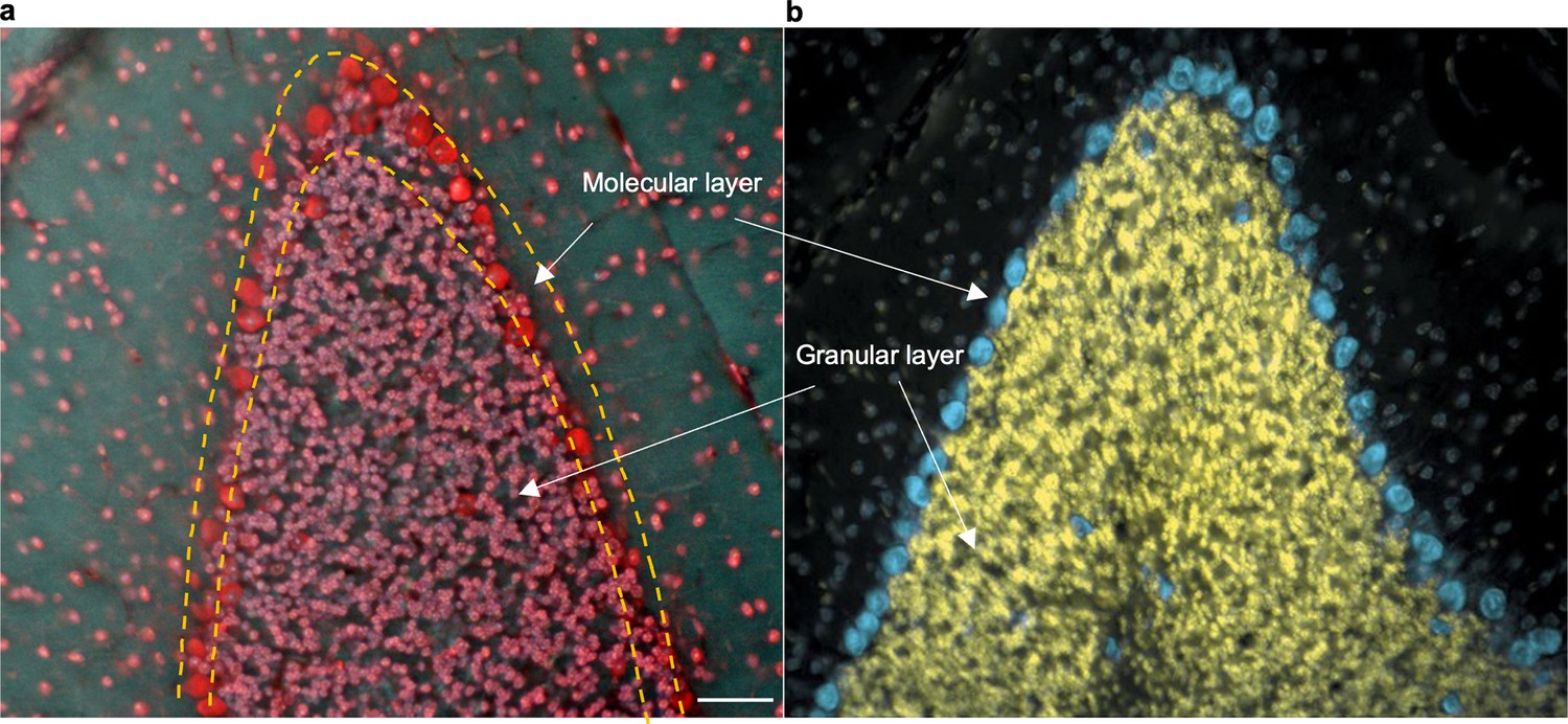
Double labeling (DAPI and PI) can serve as Nissl staining.
(a) A TRUST image of a mouse brain stained with DAPI and PI. (b), A mouse brain section stained with NeuroTrace 435/455 blue-fluorescent Nissl stain (N21479, Thermo Fisher Scientific Inc) and counterstained with nuclear yellow (N21485, Thermo Fisher Scientific Inc) Thermo Fisher Scientific Inc, 2022. Scale bar: 50 µm.
Figure 2—figure supplement 3

Cerebral vascular imaging with the assistance of intravascular perfusion.
(a), One section of the mouse brain in b has been perfused with 3% gelatine and black ink. (c), Close-up image of the blue solid region marked in a.( d), Vessels extracted from c by inverting pixel values and subsequent background subtraction. Scale bars: 500 µm (a) and 50 µm (c,d).
Figure 2—figure supplement 4
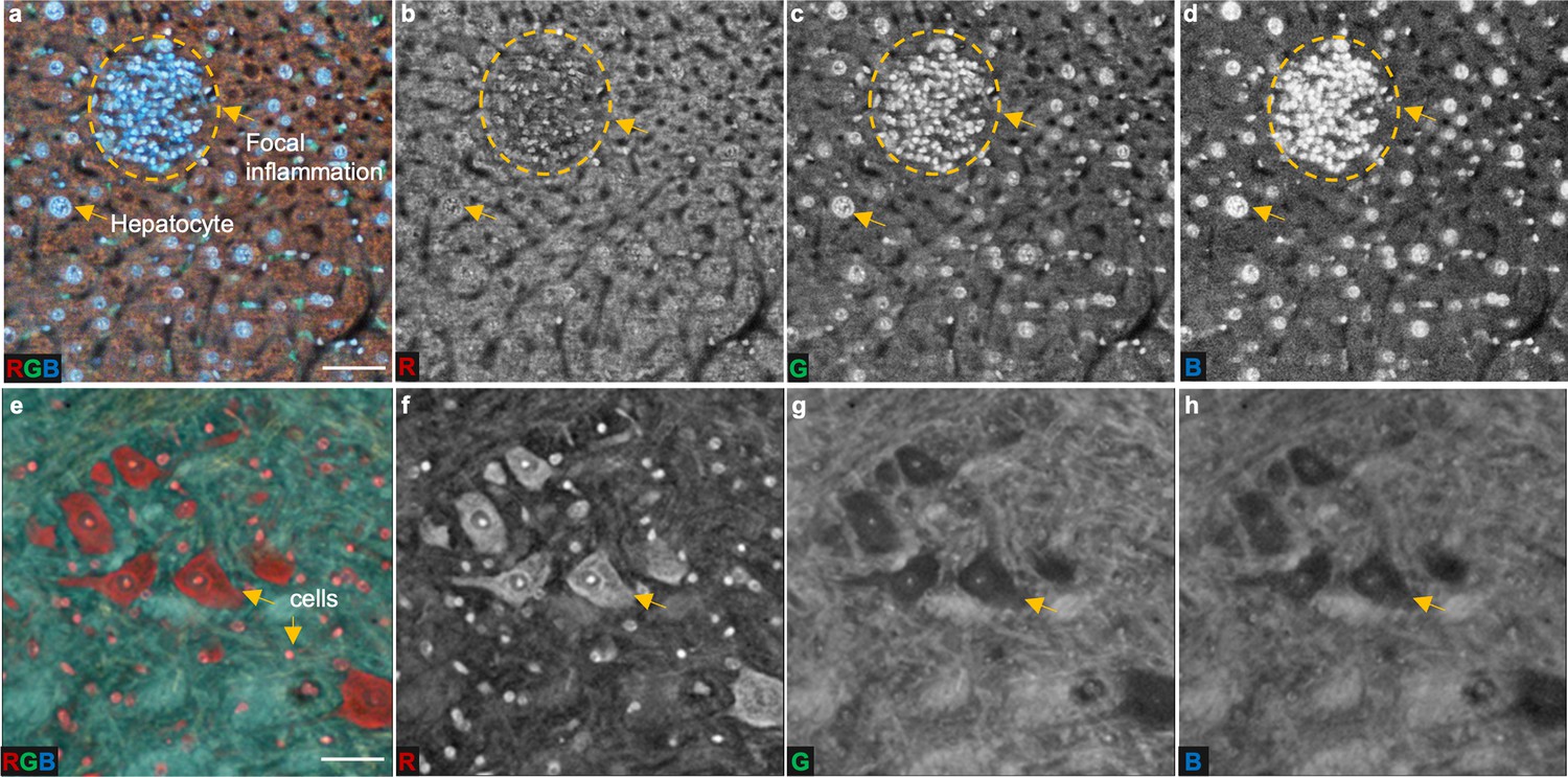
Double labeling (DAPI and PI) provides high molecular contrast from the autofluorescence background.
(a), A TRUST image of a mouse liver. (b–d), Red, green, and blue channels of a, respectively. The imaging contrast of the cell nuclei is low in the red channel since the intensity of cell nuclei labeled by PI is comparable to that of autofluorescence background. High contrast can be realized in the green or blue channels because the intensity of nuclei labeled by DAPI is higher than that of the surrounding tissue. (e), A TRUST image of a mouse brain. (f–h), Red, green, and blue channels of e, respectively. Different from the case in the mouse liver, the intensity of autofluorescence background in the red channel is lower than that of cell nuclei labeled by PI, resulting in high image contrast. However, in the green or blue channels, the nuclei labeled by DAPI cannot be clearly distinguished because the autofluorescence signal from the background is strong. Scale bars: 50 µm.
Figure 2—figure supplement 5
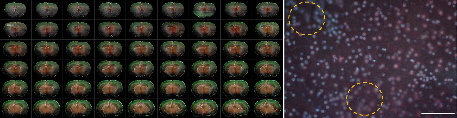
TRUST images of a fresh mouse brain.
(a), Multiple serial coronal sections of a fresh mouse brain imaged by TRUST with real-time staining by Hoechst 33342 at the concentration of 20 µg/ml. (b), One selected field of view shows out-of-focus areas of the sectioning surface due to the limited sectioning ability, as marked with yellow dashed circles. Scale bar: 100 µm.
Figure 2—video 1
3D rendering of a whole mouse brain.
Figure 2—video 2
3D rendering of the vessel network in a mouse brain.
Figure 3 with 10 supplements
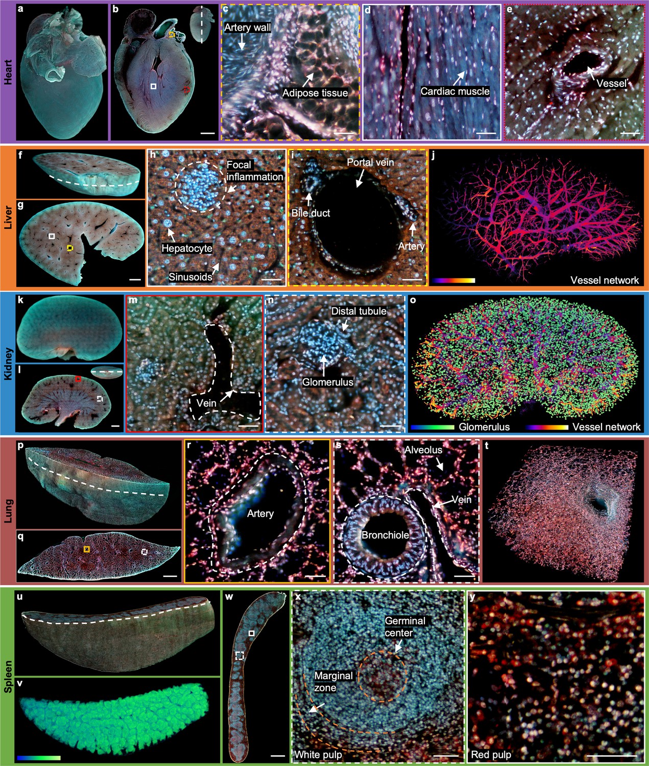
2D/3D image gallery of other organs in mice with TRUST.
(a), Reconstructed 3D model of the whole mouse heart. (b), One section of the heart with the position indicated by the white dashed line at the top right-hand corner. (c–e), Three close-up images of the orange dashed, white solid, and red dotted regions marked in b. (f), One block of a fixed mouse liver. (g), One section of the liver with the position indicated by the curved white dashed line marked in f. (h), (i), Close-up images of the white solid and yellow dashed regions marked in g. (j), Vessel network extracted based on negative contrast and rendered with pseudo color. (k), Reconstructed 3D model of a whole mouse kidney. (l), One section in the middle of the kidney with the position indicated by the white dashed line at the top right-hand corner. (m), (n), Close-up images of the red solid and white dashed regions marked in l. (o), Vessel network and glomeruli extracted from the whole kidney and rendered with pseudo color. (p), Part of a mouse lung imaged with TRUST. The curved white dashed line indicates the position of the section in q.( r), (s), Close-up images of the orange solid and white dashed regions marked in q. (t), A small zoomed-in region in p.( u), Rendered 3D model of a mouse spleen, and the curved white dashed line indicates the position of the section in w. (v), White pulp regions extracted from u through the blue channel and rendered with pseudo color. (x), (y), Close-up images of the white dashed and white solid regions marked in w. Scale bars: 1 mm (b,g,l,q,w) and 50 µm (c–e, h), (i), (m), (n), (r), (s), (x), (y).
Figure 3—figure supplement 1
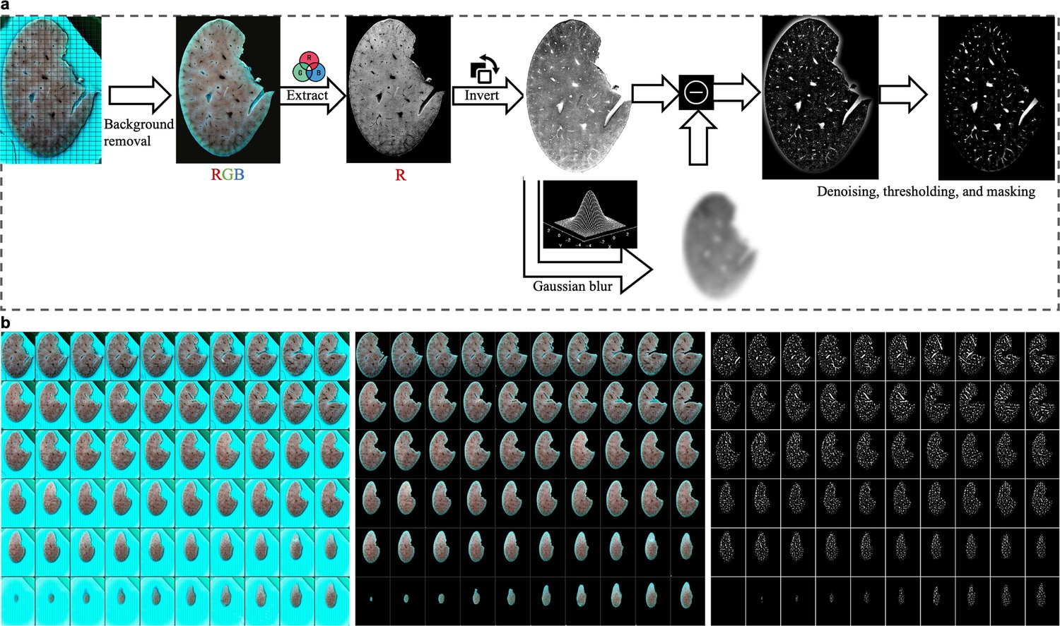
Extraction of the vascular network.
(a) Steps of image processing: background removal; extraction of the red channel; inverting the pixel value; subtracting low-frequency background to highlight the vessel structures; denoising with a median filter, thresholding, and masking. More specifically, background removal can be realized by manual masking to achieve high accuracy. The generated masks can also be utilized at the final masking step. (b), Demonstration of image processing results, taking mouse liver tissue as an example. Left: raw images; middle: images with background removal; right: final results with vessels extracted.
Figure 3—figure supplement 2
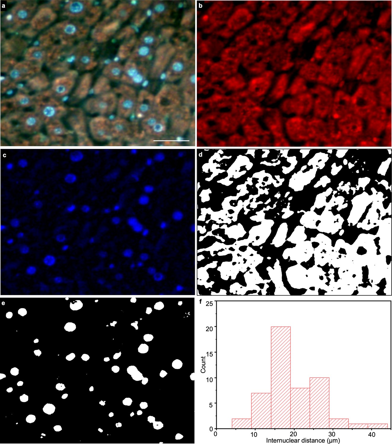
Nucleus and cytoplasm extraction from a TRUST image.
(a), One region of a mouse liver stained by DAPI & PI, which is imaged by TRUST with a 10× / 0.25 NA objective lens. (b,c) Red and blue channels of a, respectively. (d,e) Binary images generated from b and c, respectively. The nuclear/cytoplasmic ratio can be calculated as the number of white pixels in e divided by the number of white pixels in d, which is ~0.1. (f) Internuclear distance histogram generated from e based on the shortest adjacent distance to a neighboring cell nucleus. The center positions of the cell nuclei in e were determined with tools in ImageJ. Scale bar: 50 µm.
Figure 3—figure supplement 3

A mouse liver block imaged by TRUST with 10 µm z-sampling intervals.
(a), One section of a mouse liver imaged with TRUST. (b), 3D model of the liver block by stacking multiple imaged sections. Both sinusoids (orange) and cell nuclei (green) in b were rendered with pseudo color. Sinusoids were extracted with a similar method as shown in Figure 3—figure supplement 1. Cell nuclei were extracted from the blue channel with a simple contrast and threshold adjustment. Scale bars: 50 µm.
Figure 3—figure supplement 4
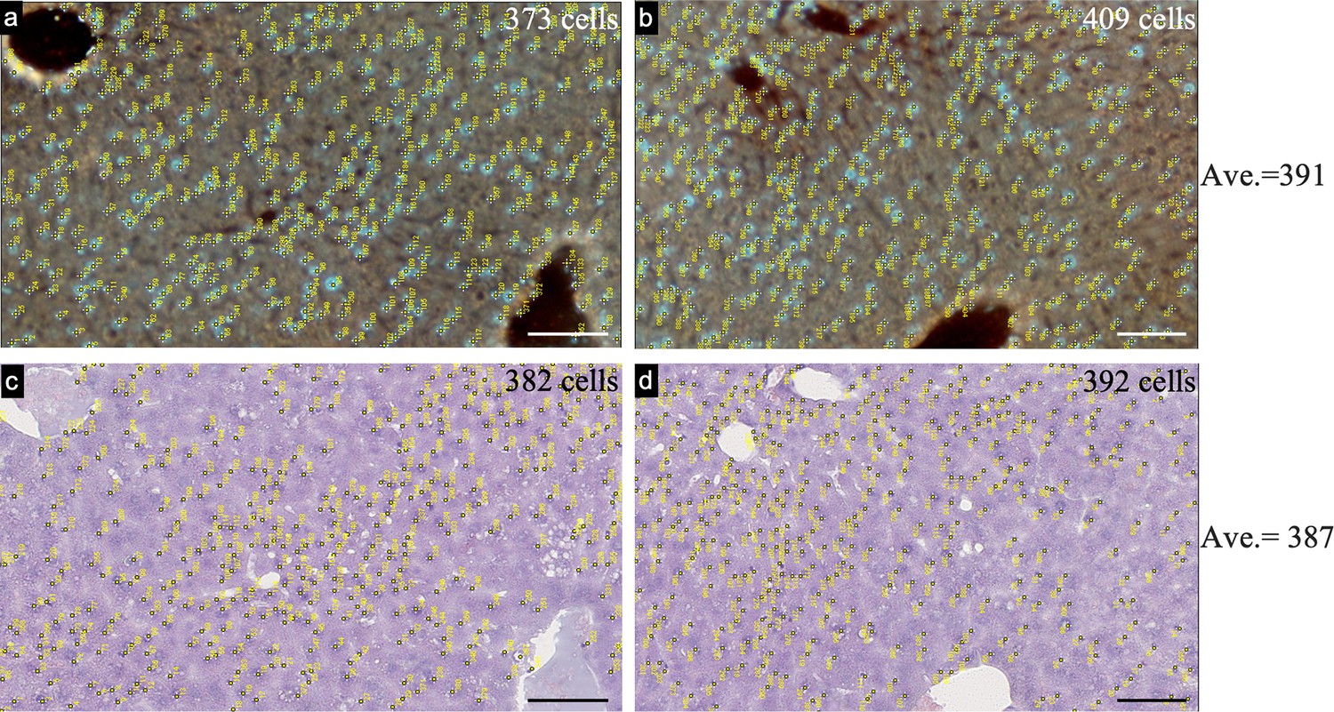
Estimation of the penetration depth of UV light by cell counting.
(a), (b), Two selected regions of the imaged surface layer of a liver block by TRUST. (c), (d), H&E stained images of the corresponding regions in a and b, respectively. The H&E stained surface layer was prepared by sectioning the previously imaged liver block with 10 µm thickness. Similar results of the cell number show that the penetration depth of UV light is around 10 µm. Scale bars: 100 µm.
Figure 3—figure supplement 5
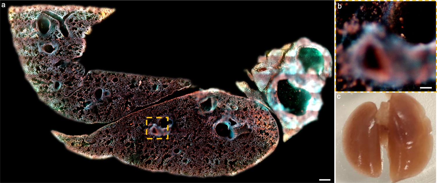
Gelatine perfusion of a mouse lung for high-quality sectioning.
(a), Uneven surface of a mouse lung sectioned by a vibratome without perfusion of gelatine. (b), Close-up image of the orange dashed region marked in a. (c), After perfusing 10% w/v gelatin through the trachea, the mouse lung is fully inflated. Gelatin can provide sufficient inner physical support to achieve high-quality sectioning performance with vibratome as shown in Figure 3—video 4. Scale bars: 1 mm (a) and 50 µm (b).
Figure 3—video 1
3D rendering of a whole mouse heart.
Figure 3—video 2
3D rendering of a whole mouse liver.
Figure 3—video 3
3D rendering of a whole mouse kidney.
Figure 3—video 4
3D rendering of a whole mouse lung.
Figure 3—video 5
3D rendering of a whole mouse spleen.
Figure 4 with 2 supplements
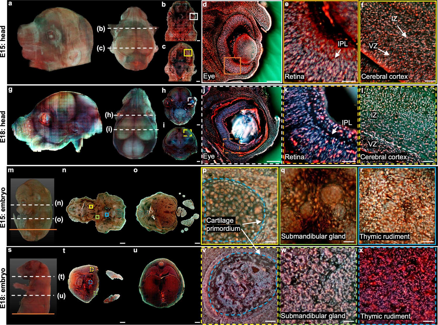
3D imaging of mouse embryos.
(a), Rendered 3D model of the embryo head at E15 viewed from two perspectives. The two white dashed lines indicate the positions of two sections in b,c. (d) Close-up image of the white solid region marked in b. (e) Close-up image of the orange solid region marked in d. (f) Close-up image of the yellow solid region marked in c. (g) Rendered 3D model of the embryo head at E18 viewed from two perspectives. The two white dashed lines indicate the positions of two sections in h,i. (j) Close-up image of the white dashed region marked in h. (k) Close-up image of the orange dashed region marked in j. (l) Close-up image of the yellow dashed region marked in i. (m) Rendered 3D model of a whole mouse embryo at E15. The two white dashed lines indicate the positions of two sections in n,o. (p–r), Close-up images of the yellow, green, and blue solid regions marked in n. (s) Rendered 3D model of a whole mouse embryo at E18. The two white dashed lines indicate the positions of two sections in t,u. (v–x) Close-up images of the yellow, green, and blue dashed regions marked in t. Scale bars: 1 mm (b,c,h,i,n,o,t,u), 500 µm (d,j), and 50 µm (e,f,k,l,p–r,v–x).
Figure 4—figure supplement 1
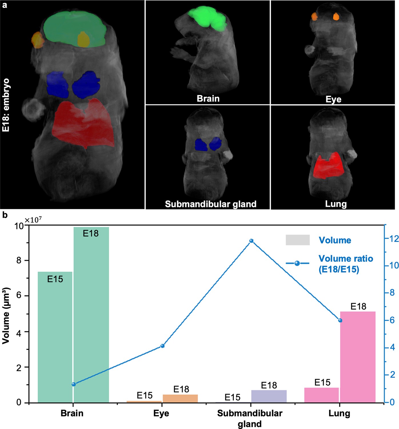
Volume quantification and comparison between embryos at different developmental stages.
(a), Rendered 3D images of the E18 embryo with the brain (green), eyes (orange), submandibular gland (blue), and lung (red) manually segmented and highlighted. (b), Volume ratio quantification of segmented organs and the submandibular gland between the E18 embryo and the E15 embryo.
Figure 4—figure supplement 2
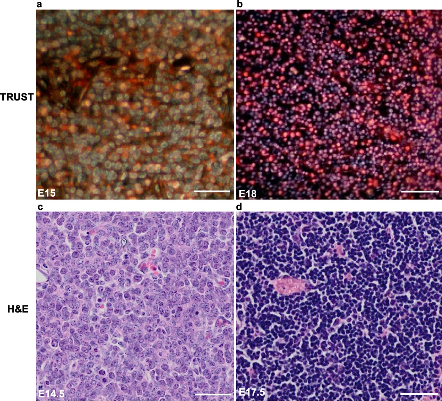
Comparison of TRUST and histological images of the thymic rudiment.
(a,b) TRUST images of the thymic rudiment from the E15 and E18 embryos, respectively. (c,d) Histological images of the thymic rudiment from the E14.5 and E17.5 embryos, respectively Matsumoto et al., 2019. Scale bars: 50 µm.
Figure 5
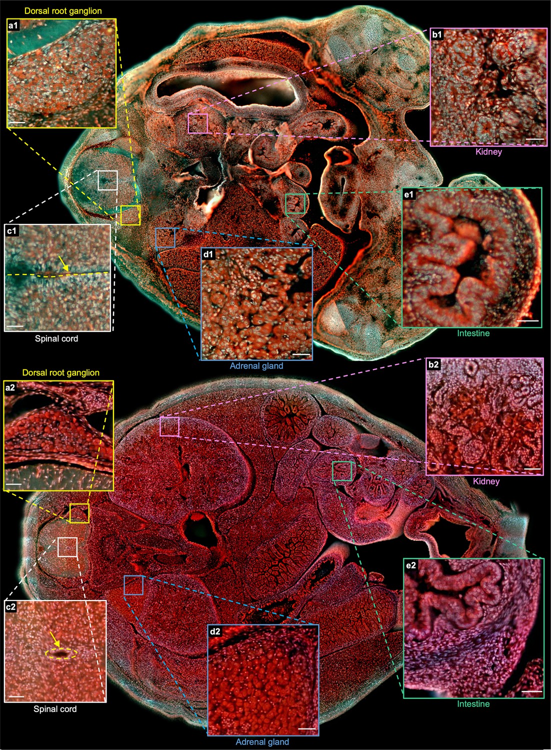
Comparison of two sections from the E15 and E18 embryos.
a1(a2)–e1(e2), Close-up images from the E15(E18) embryo of the dorsal root ganglion, kidney, spinal cord, adrenal gland, and intestine marked with yellow, pink, white, blue, and green solid boxes, respectively. Scale bars: 50 µm.
Additional files
-
MDAR checklist
- https://cdn.elifesciences.org/articles/81015/elife-81015-mdarchecklist1-v2.docx
-
Supplementary file 1
Staining and camera parameters in TRUST, and the comparison of TRUST with other whole-organ imaging modalities.
(a) Parameters of the staining solutions and the white balance. Concentrations of the staining solutions and the rates for adding additional dyes into the water tank to maintain the same concentration of the staining solutions. Note: the control of pumping rate is not necessarily needed and can be different depending on the size of the specimen and volume of the staining solutions in the water tank. The white balance (red/blue) parameters of the color camera (DS-Fi3, Nikon Corp.) in TRUST are also provided as a reference. (b) Comparison of TRUST with other whole-organ imaging modalities. The imaging speed of each modality is calculated based on the reported literature for whole mouse brain imaging, including serial two-photon tomography (STPT) Ragan et al., 2012, microtomy-assisted photoacoustic microscopy (mPAM) Wong et al., 2012, micro-optical sectioning tomography (MOST) Li et al., 2010, fluorescence micro-optical sectioning tomography (fMOST) Gong et al., 2013, light-sheet fluorescence microscopy (LSFM) Matsumoto et al., 2019, and wide-field large-volume tomography (WVT) Gong et al., 2016.
- https://cdn.elifesciences.org/articles/81015/elife-81015-supp1-v2.docx
Download links
A two-part list of links to download the article, or parts of the article, in various formats.
Downloads (link to download the article as PDF)
Open citations (links to open the citations from this article in various online reference manager services)
Cite this article (links to download the citations from this article in formats compatible with various reference manager tools)
Translational rapid ultraviolet-excited sectioning tomography for whole-organ multicolor imaging with real-time molecular staining
eLife 11:e81015.
https://doi.org/10.7554/eLife.81015


