Resource-rational account of sequential effects in human prediction
Figures
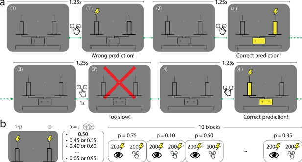
The Bernoulli sequential prediction task.
(a) In each successive trial, the subject is asked to predict which of two rods the lightning will strike. (1) A trial begins. (1’) The subject chooses the right-hand-side rod (bold lines), but the lightning strikes the left one (this feedback is given immediately after the subject makes a choice). (2) 1.25 s after the beginning of the preceding trial, a new trial begins. (2’) The subject chooses the right-hand-side rod, and this time the lightning strikes the rod chosen by the subject (immediate feedback). The rod and the connected battery light up (yellow), indicating success. (3) A new trial begins. (3’) If after 1 s the subject has not made a prediction, a red cross bars the screen and the trial ends. (4) A new trial begins. (4’) The subject chooses the left-hand-side rod, and the lightning strikes the same rod. In all cases, the duration of a trial is 1.25 s. (b) In each block of trials, the location of the lightning strike is a Bernoulli random variable with parameter , the stimulus generative probability. Each subject experiences 10 blocks of trials. The stimulus generative probability for each block is chosen randomly among the 19 multiples of 0.05 ranging from 0.05 to 0.95, with the constraint that if is chosen for a given block, neither nor can be chosen in the subsequent blocks; as a result for any value among these 19 probabilities spanning the range from 0.05 to 0.95, there is one block in which one of the two rods receives the lightning strike with probability . Within each block the first 200 trials consist in passive observation and the 200 following trials are active trials (depicted in panel a).
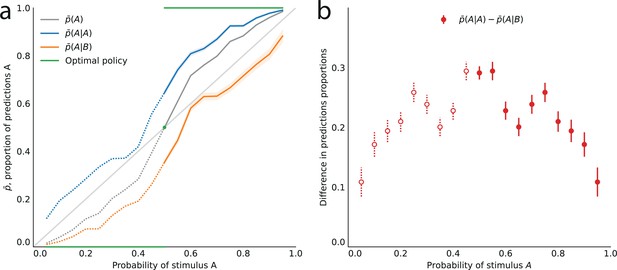
Across all stimulus generative probabilities, subjects are more likely than average to make a prediction equal to the preceding observation.
(a) Proportion of predictions A in subjects’ pooled responses as a function of the stimulus generative probability, conditional on observing an A (blue line) or a B (orange line) on the preceding trial, and unconditional (grey line). The widths of the shaded areas indicate the standard error of the mean (n = 178 to 3603). (b) Difference between the proportion of predictions A conditional on the preceding observation being an A, and the proportion of predictions A conditional on the preceding observation being a B. This difference is positive across all stimulus generative probabilities, that is, observing an A at the preceding trial increases the probability of predicting an A (p-values of Fisher’s exact tests, with Bonferroni-Holm-Šidák correction, are all below 1e-13). Bars are twice the square root of the sum of the two squared standard errors of the means (for each point, total n: 3582 to 3781). The binary nature of the task results in symmetries in this representation of data: in panel (a) the grey line is symmetric about the middle point and the blue and orange lines are reflections of each other, and in panel (b) the data is symmetric about the middle probability, 0.5. For this reason, for values of the stimulus generative probability below 0.5 we show the curves in panel (a) as dotted lines, and the data points in panel (b) as white dots with dotted error bars.
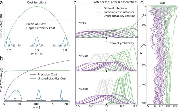
Illustration of the Bernoulli-observer models, with unpredictability and precision costs.
(a) Precision cost (purple) and unpredictability cost (green lines) of a Beta distribution with parameters and , as functions of the mean of the distribution, , and keeping the entropy constant. The precision cost is the negative of the entropy and it is thus constant, regardless of the mean of the distribution. The unpredictability cost is larger when the mean of the distribution is closer to 0.5 (i.e. when unpredictable environments are likely, under the distribution). Insets: Beta distributions with mean 0.2, 0.5, and 0.8, and constant entropy. (b) Costs as functions of the sample size parameter, . A larger sample size implies a higher precision and lower entropy, thus the precision cost increases as a function of the sample size, whereas the unpredictability cost is less sensitive to changes in this parameter. Insets: Beta distributions with mean 0.6 and sample size parameter, , equal to 5, 50, and 200. (c) Posteriors of an optimal observer (gray), a precision-cost observer (purple) and an unpredictability-cost observer (green lines), after the presentation of ten sequences of N = 50, 200, and 400 observations sampled from a Bernoulli distribution of parameter 0.7. The posteriors of the optimal observer narrow as evidence is accumulated, and the different posteriors obtained after different sequences of observations are drawn closer to each other and to the correct probability. The posteriors of the unpredictability-cost observer also narrow and group together, but around a probability larger (less unpredictable) than the correct probability. Precise distributions are costly to the precision-cost observer and thus the posteriors do not narrow after long sequences of observations. Instead, the posteriors fluctuate with the recent history of the stimuli. (d) Expected probability resulting from the inference. The optimal observer (gray) converges towards the correct probability; the unpredictability-cost observer (green) converges towards a biased (larger) probability; and the precision-cost observer (purple lines) does not converge, but instead fluctuates with the history of the stimuli.
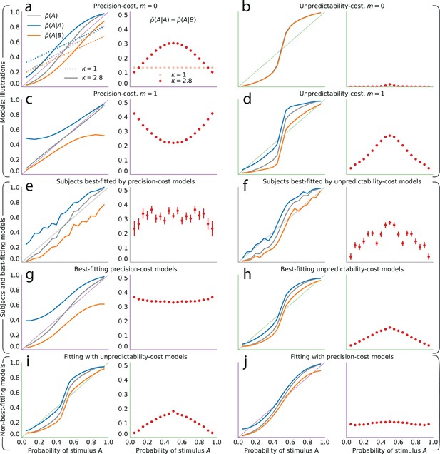
The precision-cost and unpredictability-cost models reproduce the subjects’ attractive sequential effects.
(a–h) Left subpanels: proportion of predictions A as a function of the stimulus generative probability, conditional on observing A (blue line) or B (orange line) on the preceding trial, and unconditional (grey line). Right subpanels: difference between the proportion of predictions A conditional on observing A, and conditional on observing B, . In all panels this difference is positive, indicating an attractive sequential effect (i.e. observing A at the preceding trial increases the probability of predicting A). (a–d) Models with the precision cost (a,c) or the unpredictability cost (b,d), and with a Bernoulli observer (; a,b) or a Markov observer with (c,d). (a) Behavior with the generalized probability-matching response-selection strategy with (solid lines, red dots) and with (dotted lines, light-red dots). (e,f) Pooled responses of the subjects best-fitted by a precision-cost model (e) or by an unpredictability-cost model (f). Right subpanels: bars are twice the square root of the sum of the two squared standard errors of the means (for each point, total n: e: 1393, f: 2189 to 2388). (g,h) Pooled responses of the models that best fit the corresponding subjects in panels (e,f). (i,j) Pooled responses of the unpredictability-cost models (i) and of the precision-cost models (j), fitted to the subjects best-fitted, respectively, by precision-cost models, and by unpredictability-cost models.
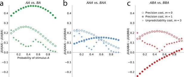
Higher-order sequential effects: the precision-cost model of a Markov observer predicts a repulsive effect of the third-to-last stimulus.
Sequential effect of the second-to-last (a) and third-to-last (b,c) stimuli, in the responses of the precision-cost model of a Bernoulli observer (; white circles), of the precision-cost model of a Markov observer with (filled circles), and of the unpredictability-cost model of a Markov observer with (crosses). (a) Difference between the proportion of prediction A conditional on observing AA, and conditional on observing BA, i.e., , as a function of the stimulus generative probability. With the three models, this difference is positive, indicating an attractive sequential effect of the second-to-last stimulus. (b) Difference between the proportion of prediction A conditional on observing AAA, and conditional on observing BAA, i.e., . The positive difference indicates an attractive sequential effect of the third-to-last stimulus in this case. (c) Difference between the proportion of prediction A conditional on observing ABA, and conditional on observing BBA, i.e., . With the precision-cost model of a Markov observer, the negative difference when the stimulus generative probability is lower than 0.8 indicates a repulsive sequential effect of the third-to-last stimulus in this case, while when the probability is greater than 0.8, and with the predictability-cost model of a Bernoulli observer and with the unpredictability-cost model of a Markov observer, the positive difference indicates an attractive sequential effect of the third-to-last stimulus.
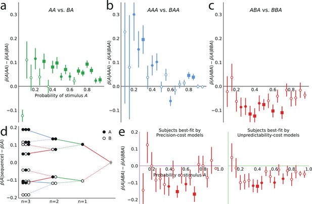
Patterns of attractive and repulsive sequential effects in subjects’ responses.
(a) Difference between the proportion of prediction A conditional on observing the sequence AA, and conditional on observing BA, i.e., , as a function of the stimulus generative probability. This difference is in most cases positive, indicating an attractive sequential effect of the second-to-last stimulus. (b) Difference between the proportion of prediction A conditional on observing AAA, and conditional on observing BAA, i.e., . This difference is positive in most cases, indicating an attractive sequential effect of the third-to-last stimulus. (c) Difference between the proportion of prediction A conditional on observing ABA, and conditional on observing BBA, i.e., . This difference is negative in most cases, indicating a repulsive sequential effect of the third-to-last stimulus. (d) Differences, averaged over all tested stimulus generative probabilities, between the proportion of predictions A conditional on sequences of up to three past observations, minus the unconditional proportion. The proportion conditional on a sequence is an average of the two proportions conditional on the same sequence preceded by another, ‘older’ observation, A or B, resulting in a binary-tree structure in this representation. If this additional past observation is A (respectively, B), we connect the two sequences with a solid line (respectively, a dotted line). In most cases, conditioning on an additional A increases the proportion of predictions A (in comparison to conditioning on an additional B), indicating an attractive sequential effect, except when the additional observation precedes the sequence BA (or its symmetric AB), in which cases repulsive sequential effects are observed (dotted line ‘above’ solid line). (e) Same as (c), with subjects split in two groups: the subjects best-fitted by precision-cost models (left) and the subjects best-fitted by unpredictability-cost models (right). In panels a-c and e, the filled circles indicate that the p-value of the Fisher exact test is below 0.05, and the filled squares indicate that the p-value with Bonferroni-Holm-Šidák correction is below 0.05. Bars are twice the square root of the sum of the two squared standard errors of the means (for each point, total n: a: 178 to 3584, b: 37 to 3394, c: 171 to 1868, e: 63 to 1184). In all panels, the responses of all the subjects are pooled together.
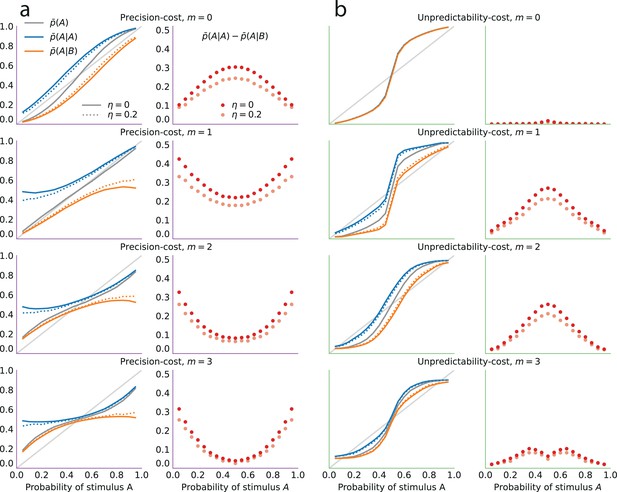
Sequential effects of the most recent stimulus in precision-cost and unpredictability-cost models.
(a) Precision-cost models. (b) Unpredictability-cost models. First row: Bernoulli observers (m = 0). Second to fourth rows: Markov observers (m = 1, 2, and 3). First column (each panel): proportion of predictions A in the models’ responses as a function of the stimulus generative probability, conditional on the preceding observation being A (blue line) or B (orange line), and unconditional (grey line); with repetition propensity (, dotted lines), and without (solid lines). Second column (each panel): difference between the proportion of predictions A conditional on the preceding observation being A, and the same proportion conditional on a B; with repetition propensity (dotted lines), and without (solid lines). A positive difference indicates an attractive sequential effect of the most recent stimulus.
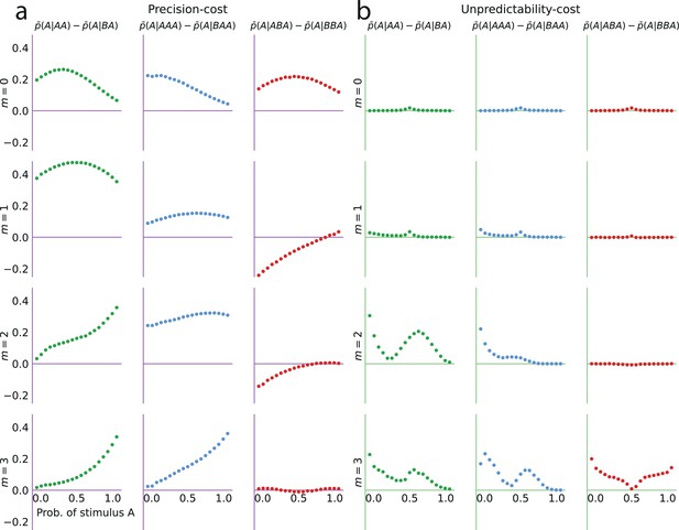
Sequential effects of the second- and third-to-last stimuli in precision-cost and unpredictability-cost models.
(a) Precision-cost models. (b) Unpredictability-cost models. First row: Bernoulli observers (m = 0). Second to fourth rows: Markov observers (m = 1, 2, and 3). First column (each panel): difference between the proportion of predictions A in the model subject’s responses, conditional on the two preceding observations being the sequence AA, and the same proportion conditional on the sequence BA. A positive difference indicates an attractive sequential effect of the second-to-last stimulus. Second column (each panel): difference between the proportion of predictions A in the model subject’s responses, conditional on the three preceding observations being the sequence AAA, and the same proportion conditional on the sequence BAA. Third column (each panel): difference between the proportion of predictions A in the model subject’s responses, conditional on the three preceding observations being the sequence ABA, and the same proportion conditional on the sequence BBA. The precision-cost models of Markov observers are the only models that yield a negative difference, i.e., a repulsive sequential effect of the third-to-last stimulus, in this case.
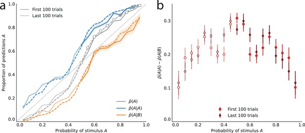
Subjects’ behavior in the first and second halves of the task.
(a) Proportion of predictions A as a function of the stimulus generative probability, conditional on observing A (blue lines) or B (orange lines), and unconditional (grey lines), in the first half of the experiment (solid lines) and in the second half (dashed lines). Filled circles indicate p-values of Fisher’s exact test (of the equality of the proportions in the first and second halves, with Bonferroni-Holm-Šidák correction) below .05. (b) Difference between the proportions of predictions A conditional on an A, and conditional on a B, in the first half of the experiment (red circles), and in the second half (dark-red diamonds). The p-values of Fisher’s exact tests (of equality of the conditional proportions, i.e., ), with Bonferroni-Holm-Šidák correction, are all below 1e-6. Bars indicate the standard error of the mean.
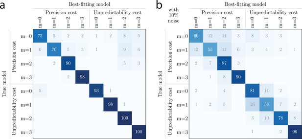
Model-fitting confusion matrix.
(a) For each row models (‘true model’), percentage of simulated datasets of 200 responses that were best fitted by column models (‘best-fitting model’). Example: when fitting data generated by the precision-cost model with , the best-fitting model was the correct model on 98% of the fits, and the precision-cost model with on 2% of the fits. (b) Same as (a), with 10% of responses (randomly chosen in each simulated dataset) replaced by the opposite responses.
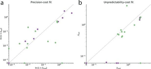
Stability of the cost-weight parameter across medium and extreme values of the stimulus generative probability.
Best-fitting parameters of individual subjects when fitting the data obtained in trials with extreme values of the stimulus generative probability (i.e., or in ), plotted against the best-fitting parameters when fitting the data obtained in trials with medium values of the stimulus generative probability (i.e., or in ), with (a) precision-cost models, and (b) unpredictability-cost models. Purple dots: subjects best-fitted by prediction-cost models. Green dots: subjects best-fitted by unpredictability-cost models. The plots are in log-log scale, except below (a) and (b), where the scale is linear (allowing in particular for the value 0 to be plotted.) For the precision-cost models, we plot the inverse of the characteristic decay time, . The grey line shows the identity function.
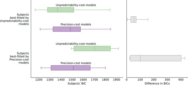
Distribution of subjects’ BICs.
(Left) Box-and-whisker plots showing the 5th and 95th percentiles (whiskers), the first and third quartiles (box), and the median (vertical line) of the BICs (across subjects) of the unpredictability-cost models (green boxes) and of the precision-cost models (purple boxes), fitted on the subjects best-fitted by the unpredictability-cost models (first two rows) and on the subjects best-fitted by the precision-cost models (last two rows). (Right) Box-and-whisker plots (same quantiles) showing the distribution of the difference, for each subject, between the BIC of the best model in the family that does not best fit the subject, and the BIC of the best-fitting model; for the subjects best-fitted by the unpredictability-cost models (top box) and for the subjects best-fitted by the precision-cost models (bottom box). The unpredictability-cost models, when fitted to the responses of the subjects best-fitted by the precision-cost models (bottom box), yield larger differences in the BIC with the best-fitting models, than the precision-cost models when fitted to the responses of the subjects best-fitted by the unpredictability-cost models (top box). This suggests that the precision-cost models are better than the unpredictability-cost models at capturing the responses of the subjects that they do not best fit.
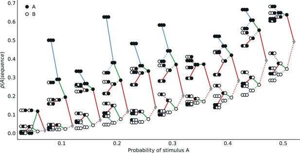
Composition of sequential effects in subjects’ responses.
Proportion of predictions A conditional on sequences of up to three past observations, as a function of the stimulus generative probability. See Figure 6d.
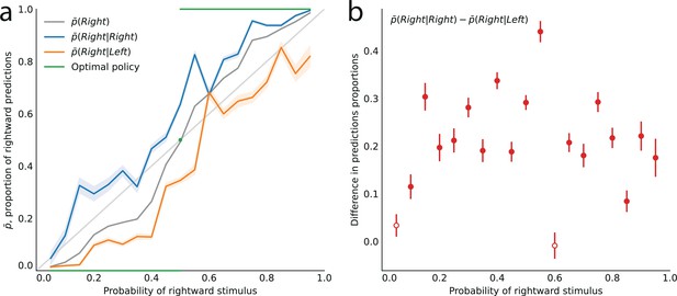
Sequential effects in subjects’ responses.
As Figure 2, but without pooling together the rightward and leftward predictions from different block of trials in which the corresponding stimuli have the same probability. See main text.
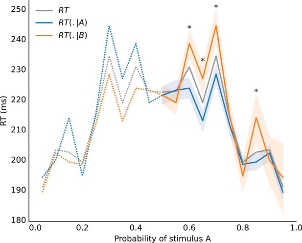
Subjects’ response times.
Average response times conditional on having observed a stimulus A (blue line), a stimulus B (orange line), and unconditional (grey line), as a function of the stimulus generative probability. The stars indicate that the p-values below 0.05 of the -tests of equality between the response times after an A and after a B. The subjects seem slower after observing the less frequent stimulus (e.g., B, when ).
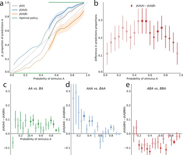
Subjects’ sequential effects — across-subjects analysis.
The statistics used for this figure are obtained by computing first the proportions of predictions A for each subject, and then computing the across-subject averages and standard errors of the mean (instead of pooling together the responses of all the subjects). (a,b) As in Figure 2, with across-subjects statistics. (c,d,e) As in Figure 6a, b and c, with across-subjects statistics. The filled circles indicate that the p-value of the Student’s t-test is below 0.05, and the filled squares indicate that the p-value with Bonferroni-Holm-Šidák correction is below 0.05.


