Granger causality analysis for calcium transients in neuronal networks, challenges and improvements
- Laboratoire de physique de l'École normale supérieure, CNRS, PSL University, France
- Spinal Sensory Signaling team, Sorbonne Université, Paris Brain Institute (Institut du Cerveau, ICM), France
Figures
Figure 1 with 7 supplements
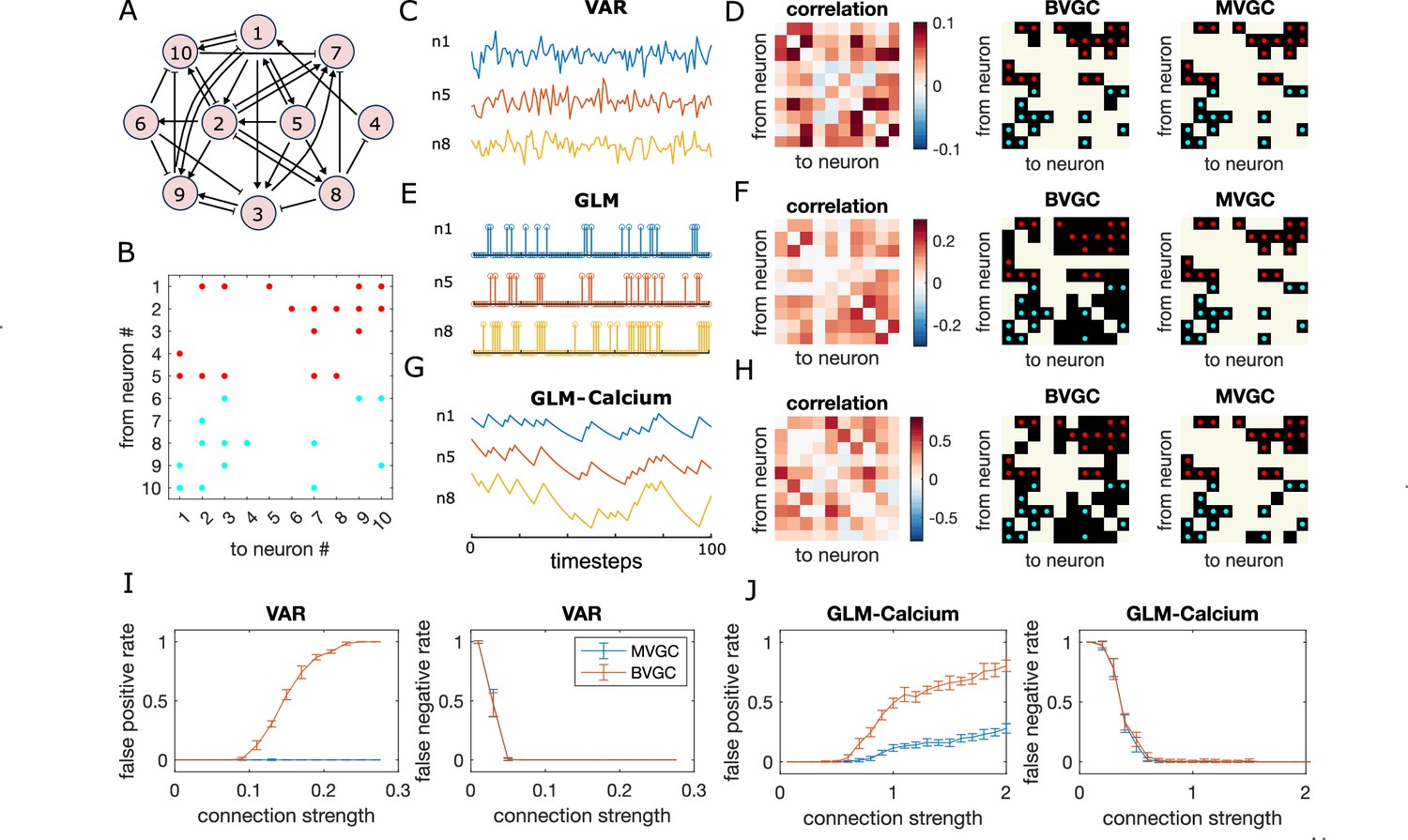
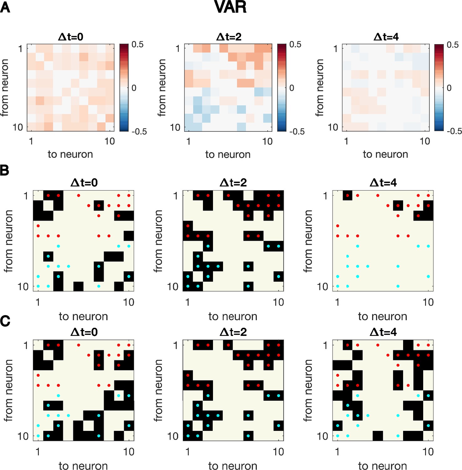
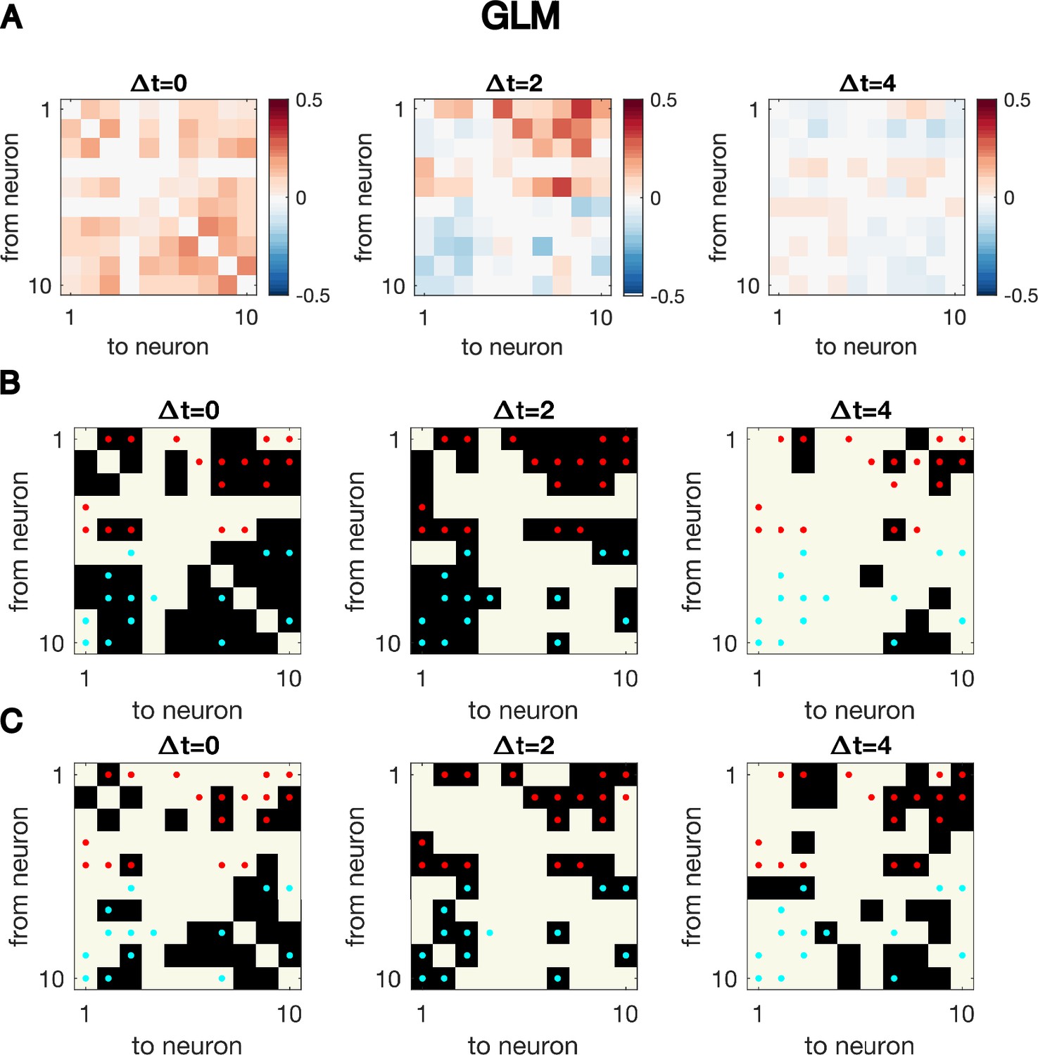
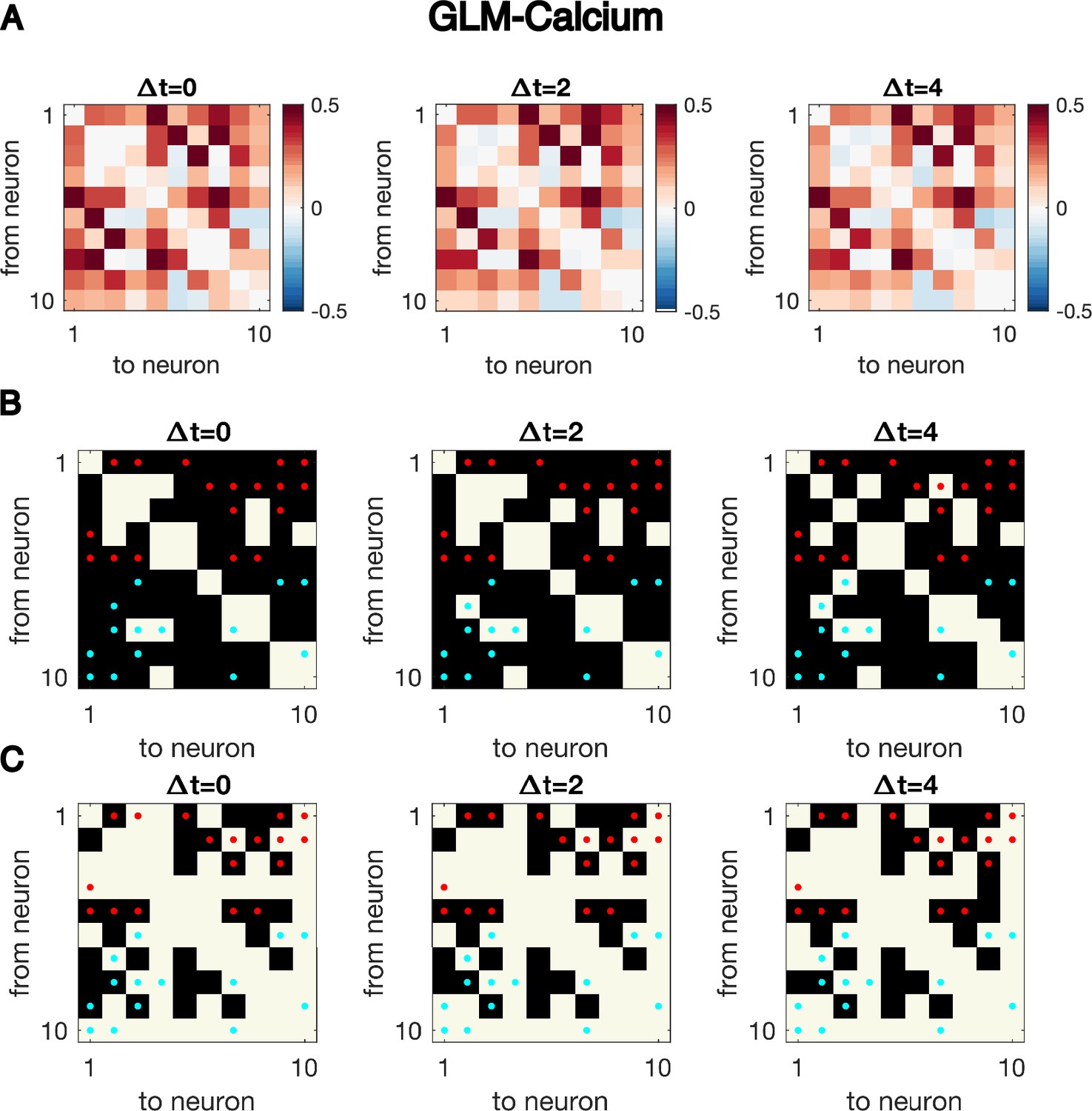
Granger causality (GC) analysis on synthetic data generated from N = 10 interconnected neurons of specific connectivity.
(A) The network diagram and (B) the connectivity matrix of the model. The excitatory links are represented by arrows in (A) and red dots in (B). The inhibitory links are represented by short bars in (A) and blue dots in (B). Time series are generated and analyzed using correlation analysis and GC, using either a vector autoregressive (VAR) process with connection strength (C–D), a generalized linear model (GLM) with connection strength (E–F), and a GLM with calcium filtering as in the experiments (G–H). (D,F,H) Comparison performance of correlation analysis using trajectory simulated with T = 5000 timepointes, bivariate (BVGC) and multivariate (MVGC) GC in predicting the connectivity matrix. True connectivity are indicated with red dots for excitatory links and blue dots for inhibitory links. The error rate of connectivity identification varies as a function of interaction strength for both the VAR dynamics (I) and the GLM-calcium-regressed dynamics (J). The multivariate GC always does better at predicting true connectivities than the bivariate (pairwise) GC and than correlation analysis. Error bars in (I) and (J) are standard deviation across 10 random realizations of the dynamics, each lasting T = 5000 timepoints.
Figure 1—figure supplement 1
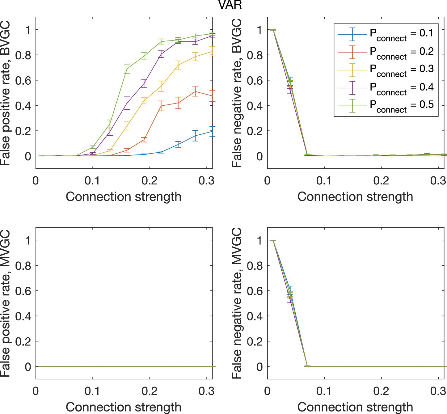
The error rate of connectivity detection as a function of connection strength and the probability of connection , for VAR dynamics on randomly connected networks of 10 neurons.
The error rate of connectivity detection as a function of connection strength and the probability of connection , for VAR dynamics on randomly connected networks of N = 10 neurons. Error bars are standard deviation across 20 random realizations of random networks, each with a single simulated trajectory of T = 5000 time points.
Figure 1—figure supplement 2
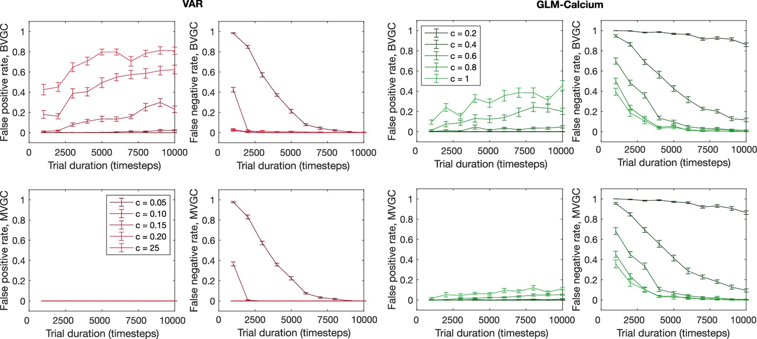
The error rate of connectivity identification as a function of trial duration and connection strength.
The error rate of connectivity identification varies as a function of trial duration and connection strength for VAR and GLM-Calcium dynamics for random networks of N = 10 neurons. Error bars are standard deviation across 10 random realizations of the randomly connected network.
Figure 1—figure supplement 3
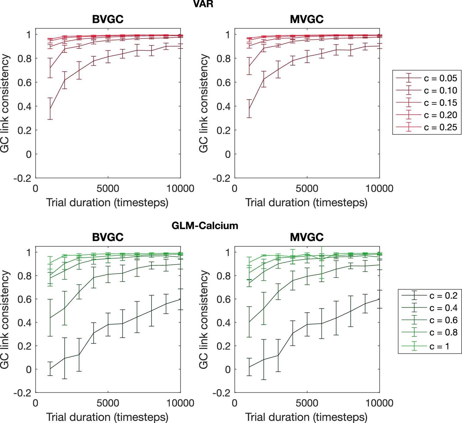
The consistency of GC values as a function of trial duration and connection strength.
The consistency of GC values as a function of trial duration and connection strength for VAR dynamics simulated on random networks of N = 10 neurons. We measure the consistency of GC values using the Pearson’s correlation coefficient between GC values computed from two realizations of synthetic data generated using the same underlying dynamics. The consistency always improves with longer trial duration and stronger connection strength and is in general better for time series generated using VAR dynamics compared to the ones generated using the non-linear non-gaussian GLM-Calcium dynamics. Error bars are standard deviation across 10 random realizations of the network.
Figure 1—figure supplement 4
Cross-correlation analysis for synthetic data generated with VAR dynamics reveals the correct interaction structure at the exact delay time difference.
Cross-correlation analysis for synthetic data generated with VAR dynamics reveals the correct interaction structure at the exact delay time difference. Here, N = 10 neurons are simulated for T = 5000 time points, the same simulated trajectory as the one used to plot Figure 1CD. (A) Cross-correlation matrix at The true underlying dynamics has neuron-neuron interaction for (B) Significant cross-correlations are marked by black squares, while the true underlying network is indicated by red dots. (C) Links with top absolute value of cross-correlations, with the number of total links matching that of the true underlying connectivity.
Figure 1—figure supplement 5
Cross-correlation analysis for synthetic data generated with GLM dynamics over-identifies connections.
Same as Figure 1—figure supplement 4, but for synthetic data generated using GLM dynamics with N = 10 neurons for T = 5000 time points, the exact same simulated dynamics as used to plot Figure 1EF. Even at the true time difference, , the significant cross-correlation over-identifies true connectivity.
Figure 1—figure supplement 6
Cross-correlation analysis for synthetic data generated with the GLM-Calcium dynamics cannot identify the underlying structure of connectivity.
Same as Figure 1—figure supplement 4, but for synthetic data generated using GLM-calcium dynamics with N = 10 neurons for T = 5000 time points, the exact same simulated dynamics as used to plot Figure 1GH. Cross-correlation cannot identify the underlying structure of connectivity.
Figure 1—figure supplement 7
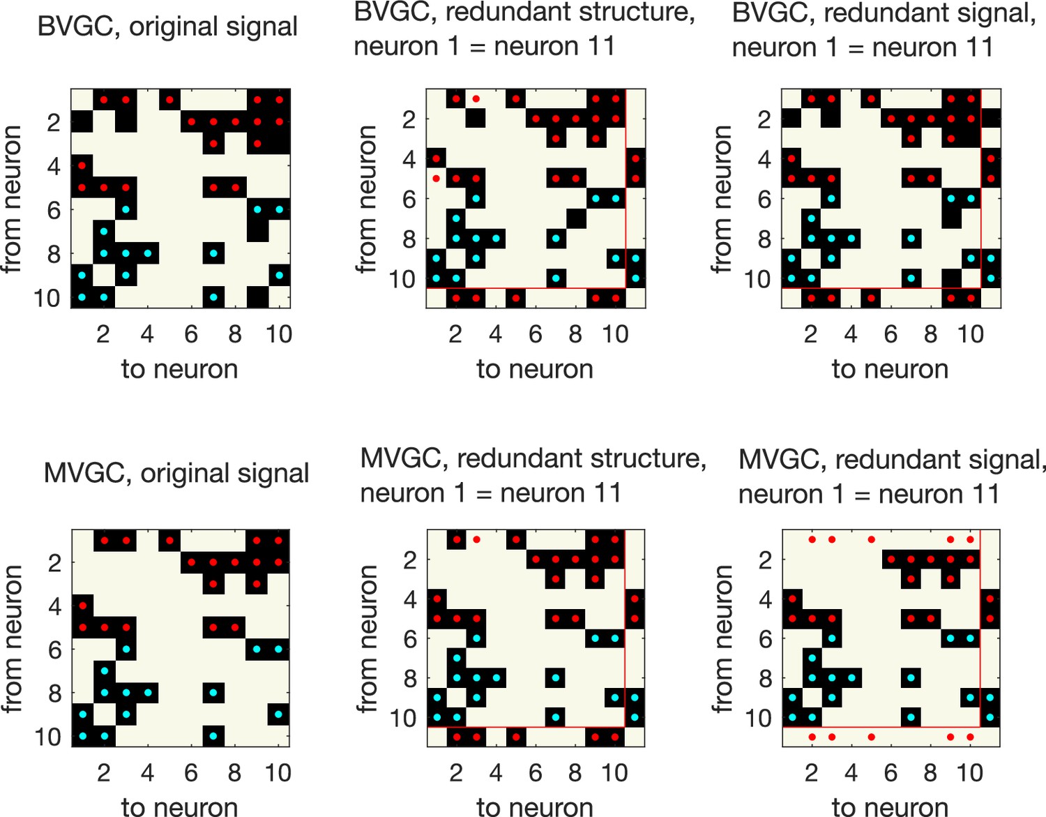
Presence of redundant signals harms the performance of MVGC.
Presence of redundant signals harms the performance of MVGC. GC analysis performed on synthetic data generated using VAR dynamics on the network structure in the main figure, for N = 10 neurons for data points. GC reveals all links for networks with redundant structures, where an ‘artificial’ neuron 11 is created with identical input and output strength as neuron 1 (redundant structure, middle column). However, MVGC fails to identify causal links when the signal from neuron 1 is copied to create another ‘artificial’ neuron 11 (redundant signal, right most column). BVGC is able to identify the underlying true connectivity.
Figure 2 with 2 supplements
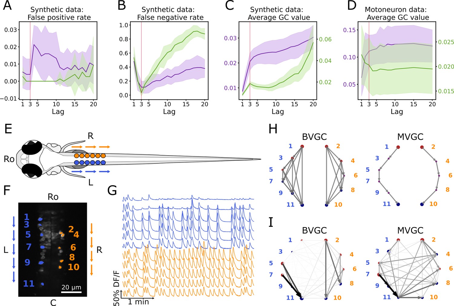
Bivariate and multivariate GC analyses of motoneuron calcium imaging recordings in a zebrafish embryo do not match expected ipsilateral and rostral to caudal information flow.
(A) Effect of the maximum lag on the false positive rate, that is the proportion of spurious positive links over all negative links, on synthetic data (VAR) with a true lag of 3, for BVGC (purple) and MVGC (green). BVGC is more prone to detect spurious links, even at the correct lag. (B) The false negative rate, that is the proportion of missed positive links over all positive links, is very sensitive to the choice of the lag. If the chosen lag is very different compared to the true lag, many links will not be detected. (C,D) Effect of the lag on the average GC values for synthetic (C) and real motoneuron (D) data (N = 11 neurons, De Vico Fallani et al., 2014). Using the average GC value, we choose a lag of 3 for the motoneuron data analysis, corresponding to 750ms. Further supporting evidence for choosing is given by the correlation analysis of GC values using different lags in Figure 1. Error bars in (A), (B) and (C) are standard deviation across 10 random realizations of the simulated dynamics with T = 4000 on the network (N = 10 neurons) specified by Figure1A. Error bars in (D) correspond to the standard deviation of the average GC value across the ten recordings of the motoneuron dataset. (E) Dorsal view of the embryonic zebrafish and positions of the left (L) and right (R) motoneurons targeted in calcium imaging (colored circles). The arrows represent the wave of activity, propagating ipsilaterally from the rostral (Ro) spinal cord to the caudal (C) spinal cord. (F) Mean image of a 30-somite stage embryonic zebrafish Tg(s1020t:Gal4; UAS:GCaMP3), dataset f3t2 in De Vico Fallani et al., 2014, with motoneurons selected for analysis shown in color. (G) Fluorescence signals (proxy for calcium activity) of selected neurons. We observe an oscillating pattern of activation of the left vs right motoneurons. (H) Representation of the motorneuron flow of information as a directed graph as would be ideally defined by bivariate (left) and multivariate (right) GC analyses. (I) Resulting directed networks for bivariate (left) and multivariate (right) GC analyses of fluorescence traces of (G) at maximum lag : we observe different networks than expected, both for BVGC and MVGC. This is consistent with the effect observed in (A), that BVGC detects many spurious links.
Figure 2—figure supplement 1
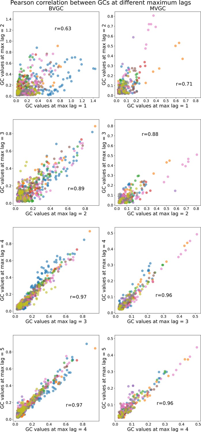
Comparison of Granger causality analysis results at different maximum lags.
Comparison of Granger causality analysis results at different maximum lags. Correlation between the GC values obtained for each pair of neurons using max lag and max lag . All fish (n=9) of the motoneuron data set are used and represented by color (same as in Figure 7). The similarity in Granger causality values, measured by the Pearson correlation coefficient , increases as increases and then stabilizes after maximum lag ( both for BVGC and MVGC between and , as well as between and ), justifying our decision to use . Using a larger maximum lag does not bring more information but brings more complexity, and increases the computation time (especially for MVGC).
Figure 2—figure supplement 2
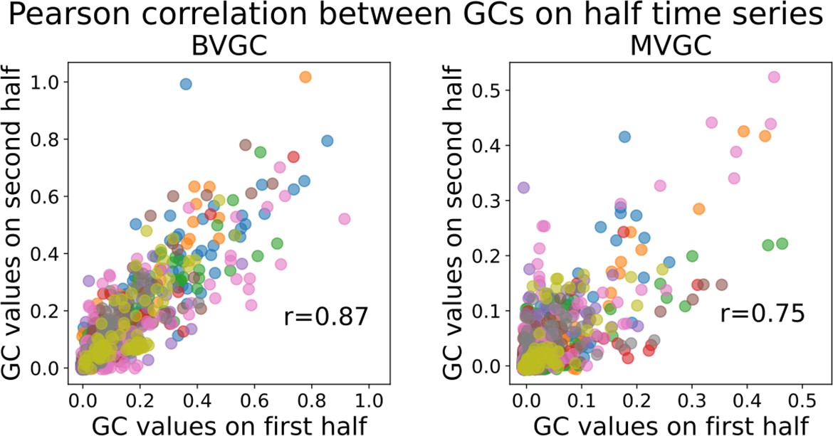
Validation of trial length sufficiency by high correlation of Granger causality values using the first and second halves of the motoneuron data.
Validation of trial length sufficiency by high correlation of Granger causality values using the first and second halves of the motoneuron data. Correlation between the GC values obtained for each pair of neurons using either the first or the second half of the calcium traces. Each color represents a different fish (n=9). The BVGC (left) and MVGC (right) results are similar (Pearson correlation coefficient) suggesting that the length of the whole time series (1000 time steps) is sufficient and appropriate to apply GC analysis (on smoothed , motion artifacts removed). The correlation is particularly for the number of time points and neurons high due to the cyclic pattern of neuronal activity leading to two very similar halves.
Figure 3 with 1 supplement
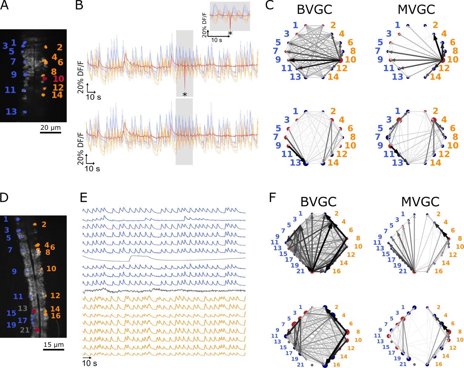
One time-point artifact or one noisy neuron fluorescence trace is sufficient to corrupt the GC algorithm.
(A) Mean image of a 30-somite stage larval zebrafish Tg(s1020t:Gal4; UAS:GCaMP3), dataset f3t1 in De Vico Fallani et al., 2014, with neurons selected for analysis shown in color. (B) Fluorescences traces of neurons of (A). Top: A motion artifact consisting of a drop in fluorescence at a single time point is present (star). Bottom: the motion artifact is corrected as being the mean of the two surrounding time points. (C) Directed graph resulting from the bivariate (left) and multivariate (right) GC analysis, before (top) and after (bottom) motion artifact correction. Before the correction, the neuron with the smallest activity appears to drive many other neurons, perhaps due to its lower SNR. This spurious dominant drive disappears once the motion artifact is corrected, demonstrating that GC is not resilient to artifacts as small as one time point out of one thousand. (D) Mean image of a 30-somite stage larval zebrafish Tg(s1020t:Gal4; UAS:GCaMP3), dataset f5t2 in De Vico Fallani et al., 2014, with neurons selected for analysis shown in color. The fluorescence traces (E) of neurons displayed in red exhibit activity patterns different from the oscillatory pattern expected in motorneurons. GC analysis was run after removal of these neurons. (F) Directed graph resulting from the bivariate (left) and multivariate (right) GC analysis, before (top) and after (bottom) removing neuron 13 and neuron 21.
Figure 3—figure supplement 1
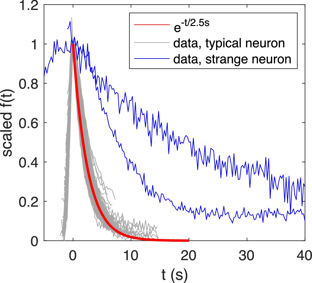
Re-scaled calcium transients exhibits a typical exponential decay with time constant , while atypical transients exhibit a slower decay.
Overlaid and re-scaled calcium signals from the motoneuron experiment (dataset f5t1 from De Vico Fallani et al., 2014) shows the typical decay of calcium transients (overlay of calcium transients from 4 neurons) can be well approximated by an exponential function with time constant , while atypical calcium transients exhibit a slower decay.
Figure 4 with 4 supplements

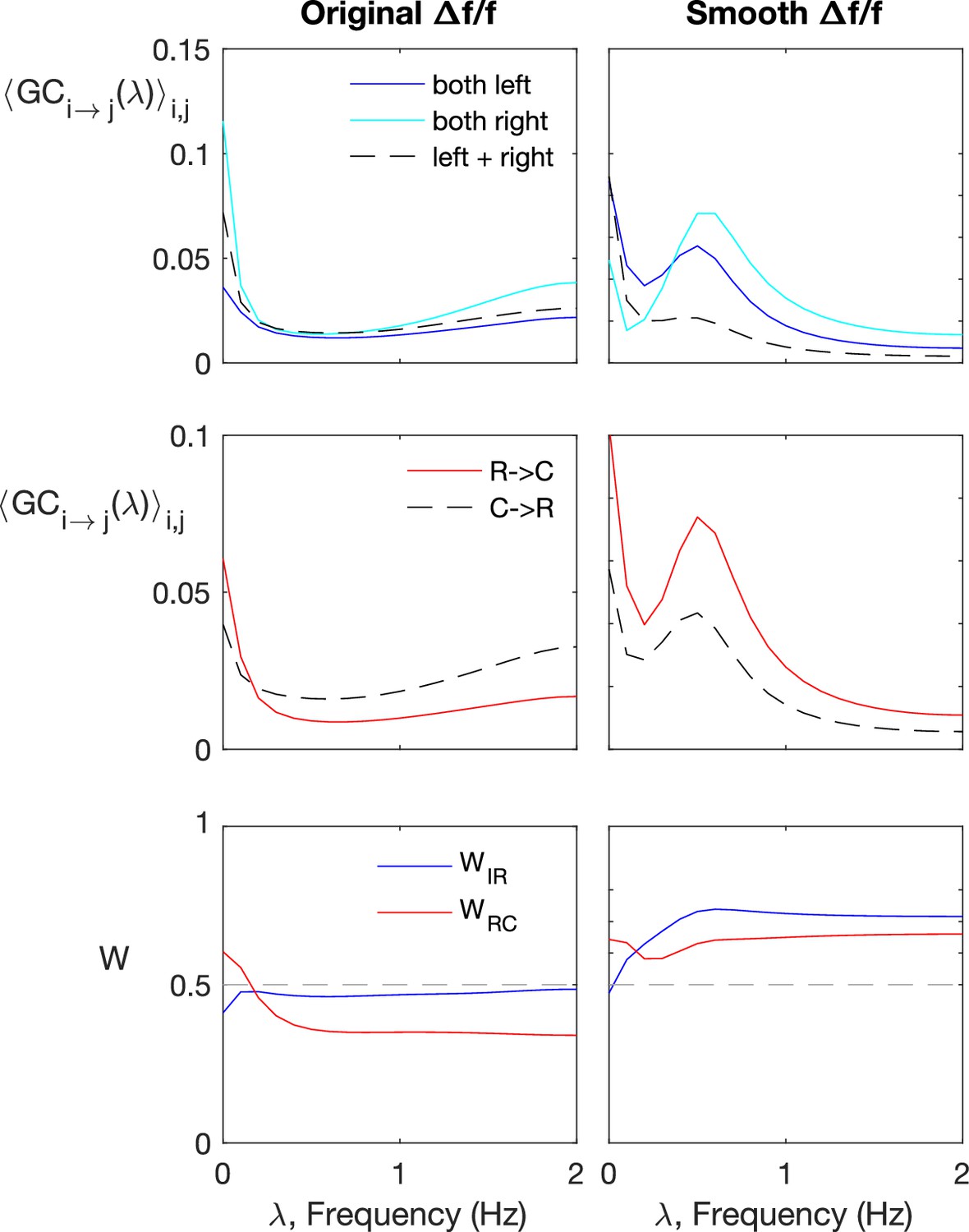
Smoothing the calcium imaging signal can improve the accuracy of GC.
(A) We smooth the noisy calcium imaging signal using total-variational regularization (see Materials and Methods), and plot the example traces of the original and the smoothened neuronal signals, and the residual noise, using the dataset f3t2 (N = 11 neurons) from De Vico Fallani et al., 2014. (B) The Pearson correlation coefficient shows the residual noise is correlated. (C) GC networks constructed using the original noisy calcium signal compared to ones using the smoothed signal for motorneurons. (D) Weight of ipsilateral GC links, , and the weight of rostal-to-cordal links, , for the original calcium signals and smoothened signals. We expect and a null model with no bias for where the links are placed will have . The x-axis is sorted using the value for bivariate GC analysis with the original calcium data. Data points are connected with lines to guide the eye. The bivariate GC results are plotted with purple circles, and the multivariate GC results with green diamonds. GC analysis results using the original noisy fluroscence signals are shown with empty markers, while the results from first smoothed data are shown with filled markers.
Figure 4—figure supplement 1
Cross-correlation of the residual noise after smoothing.
The Pearson correlation coefficient shows that the residual noise carries signals of information flow, after the original calcium signals are smoothen, using the dataset f3t2 from De Vico Fallani et al., 2014 as an example (N = 11 neurons). Top-left panel is identical as Figure 4B.
Figure 4—figure supplement 2
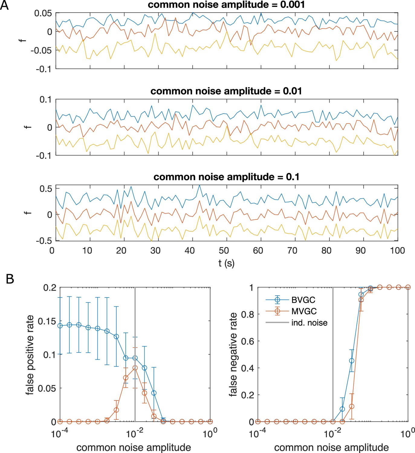
Correlated noise increases the error of Granger causality analysis for synthetic data generated by VAR dynamics.
Correlated noise increases the error of Granger causality analysis, exemplified by synthetic data generated by VAR dynamics and corrupted by a system-wide shared noise for N = 10 neurons and T = 4000 time points, with connection strength c = 0.1265. (A) Example traces for VAR dynamics added with shared noise with increasing strength. (B) The error of GC analysis increases as the amplitude of the shared noise increases. Error bars are standard deviation across 10 random simulated trajectories of the same network, each corrupted by adding a realization of randomly generated noise.
Figure 4—figure supplement 3
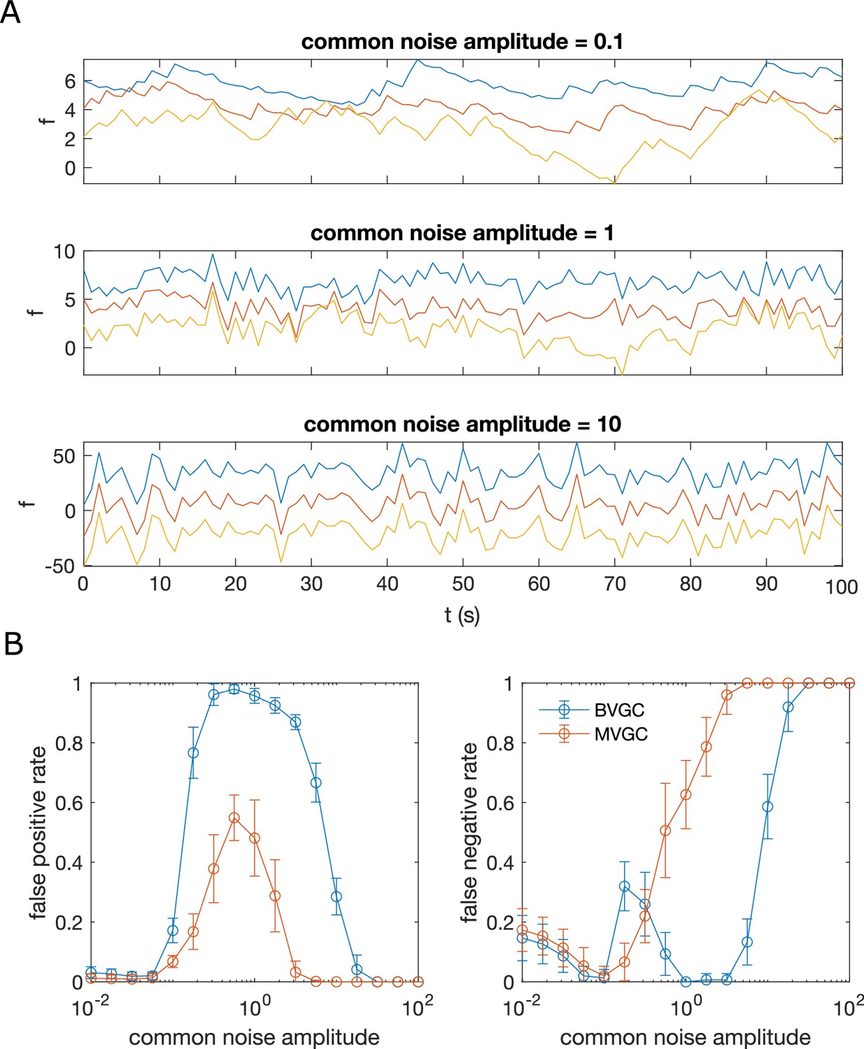
Correlated noise increases the error of Granger causality analysis for synthetic data generated by GLM-calcium dynamics.
Same as Figure 2, but for data generated with GLM-calcium dynamics for N = 10 neurons, a connection strength of c = 1, and for duration T = 4000. Error bars are standard deviation across 10 realizations of simulation.
Figure 4—figure supplement 4
Spectral Granger-causality does not improve information flow detection for the original, not pre-smoothened data.
Spectral Granger-causality (computed using the Barnett and Seth, 2014). Results for motoneurons (dataset f6t1, N = 12 neurons) reveals more structre when applied to smoothened fluorescence data compared to the raw fluorescence signal. The top row shows the ipsilatarel links in solid curves, and contralateral links in dashes. The top row shows the rostral-to-caudal links in solid curves, and caudal-to-rostral links in dashes. The last row shows the weighted ipsilateral ratio and the weighted rostral-to-caudal ratio .
Figure 5
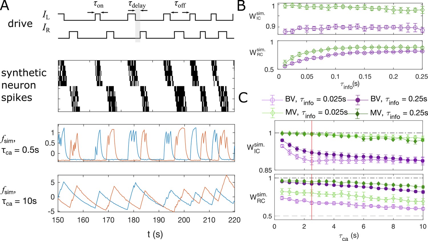
Synthetic data mimicking bursting motoneurons shows the slow timescale of calcium signal decay decreases GC performance.
(A) Example traces of the synthetic data for two chains of five neurons (N = 10 neurons for the whole system). The common stimuli, and , are sampled using the empirically observed on- and off-durations for the neuron bursts ( and ). The time delay of the onset of the right stimulus from the offset of the left stimulus is also sampled using empirical distribution. Each synthetic data is generated for the duration of 1000s. (B) Success of information flow retrieval, measured by the weight of the ipsilateral GC links, , and the weight of rostral-to-caudal links, , as a function of the information propagation time scale , evaluated at the empirical time scales , , and biologically reasonable base spike rate . Results from bivariate GC are plotted in purple, and results from multivariate GC are in green. (C) Success of information flow retrieval for and for synthetic data with different calcium decay time constants. Greater calcium decay constants lead to worse information retrivals. Errorbars represents standard deviations across 10 realizations of synthetic data. The empirical calcium time scale is indicated by the red vertical line. Error bars in panel (B) and (C) are standard deviation across 10 random realizations of the synthetic data.
Figure 6
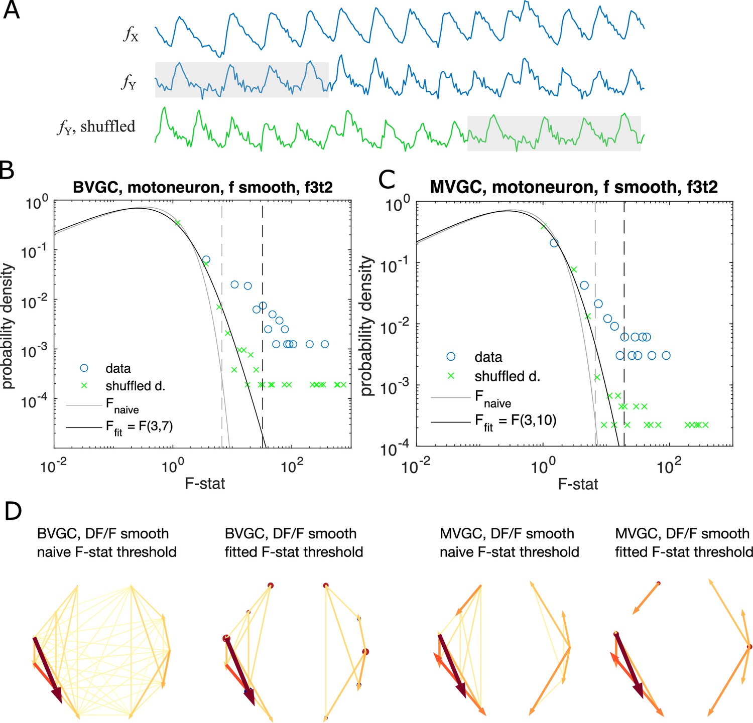
Significance tests for Granger causality on real calcium data require new thresholds, generated using null models.
(A) Schematics for generating null models by randomly shuffling the data. The blue dots and curves correspond to the original data, the effect neuron and the cause neuron ; the green ones are generated by random cyclic shuffling of the original , with gray rectangles indicating matching time points before and after the cyclic shuffle. (B) The probability density of the F-statistics of the bivariate Granger causality for an example experiment (dataset f3t2 from De Vico Fallani et al., 2014 with N = 10 neurons). Blue circles are computed using the smoothed Calcium signals, and the green crosses are computed using the null model generated with cyclic shuffles. The black curve is the F-distribution used in the naive discrimination of GC statistics, and the gray curve is the best fitted F-distribution, fitting an effective number of samples. The gray and the black dashed vertical lines indicate the significance threshold for Granger causality, using the original threshold and the fitted threshold, respectively. (C) Same as (B), for multivariate Granger causality analysis. (D) Comparison between the significant GC network for the experiment f3t2 using the naive vs. fitted F-statistics threshold.
Figure 7
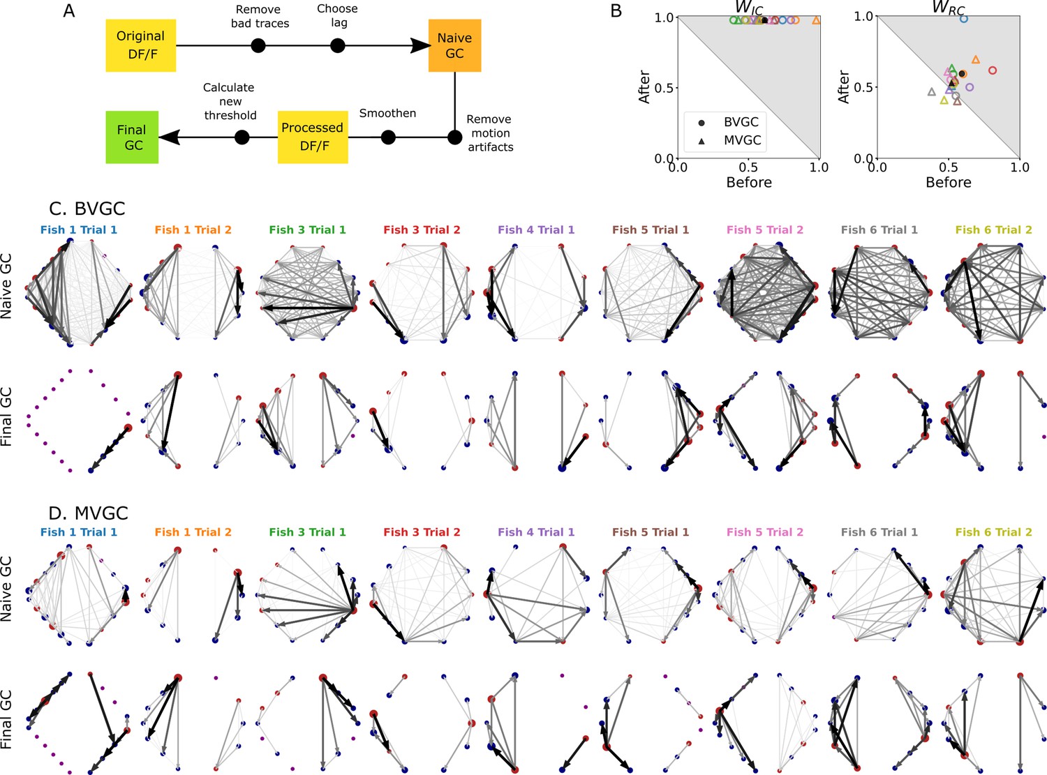
Comparison of GC analysis results with and without processing the calcium transients and adapting the threshold.
(A) Description of the whole pipeline. Before running the GC analysis on the raw calcium transients (), the lag parameter must be chosen. Then, before running the GC analysis again, motion artifacts are corrected, the fluorescence is smoothed and a new threshold is calculated. (B) Comparison of and before and after applying the pipeline to the GC analyses. Points in the upper right triangle gray-shaded area represent the ratios that have increased in the final GC results. Each fish (n=9) is represented by a color, BVGC by circles and MVGC by triangles. Means are shown in black. We find that using our pipeline, strongly increases and we can clear out the spurious contra-lateral links present in the original GC. is not significantly improved: the recording frequency and GCaMP decay are likely too low and slow compared to the speed of rostro-caudal propagation of the information flow. (C) Network results before (top row) and after (bottom row) applying our pipeline for computing bivariate Granger causality (BVGC), for all fish. For consistency in the network representation and better ability to compare, we removed the uncharacteristically behaving neurons of the GC analysis before applying the pipeline. Note that more links are found on the side that was better in focus in the recording. (D) Same as (C) but for the multivariate Granger causality (MVGC).
Figure 8 with 5 supplements
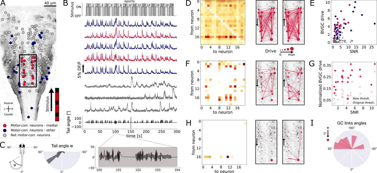
Our Granger causality pipeline revealed revealed right-to-left information flow among motor-correlated hindbrain neurons in larval zebrafish performing optomotor (OMR) responses.
(A) Two-photon laser scanning calcium imaging in vivo was acquired at 5.81Hz in the hindbrain of Tg(elavl3:GCaMP5G) transgenic larvae performing OMR (data from Severi et al., 2018). Forty-one (red and blue) out of 139 neurons from a reference plane of a larval zebrafish hindbrain were motor-correlated and selected for subsequent analysis. Neurons located in the medial area (red, N = 20 neurons) are in the location of the V2a reticulospinal stripe (Kinkhabwala et al., 2011), distinct from other motor-correlated neurons (blue, N = 21). The activity of all other neurons (gray, N = 98 neurons) were not correlated to the motor output. (B) Sampled calcium traces of the three categories of neurons mentioned above were ordered by decreasing signal-to-noise ratio (SNR) from top to bottom. The moving grading (top trace) was presented to the right of the fish from tail to head to induce swimming, depicted as the tail angle (bottom trace, with a zoom over 4s showing two subsequent bouts, positive tail angles correspond to left bends). (C) The distribution of the tail angles for turns (tail angle with ) was biased to the left. (D) GC matrix (left) and map of information flow (right, the arrows indicate the directionality of the GC links) for the naive BVGC on medial motor-correlated neurons. Of the 380 possible pairs, 351 were found to have a significant drive, suggesting that the naive BVGC algorithm is too permissive to false positive links, and justifying an adapted pipeline to remove spurious connections. (E) The neuronal drive, calculated as the sum of the strength of all outgoing GC links for each neuron, was correlated to the SNR of the calcium traces, especially high for medial neurons (, compared to across all 139 neurons). (F) Customization of the threshold and normalization of the GC values reduced the number of significant GC links and revealed numerous commissural links that were both rostrocaudal and caudorostral between medial motor-correlated neurons. (G) The new neuronal drive was less correlated with the SNR (from 0.69 to 0.49 for medial neurons). (H) Due to the high correlation in the selected neurons and the relatively high number of neurons (20), the new MVGC pipeline highlighted only the strongest GC links. (I) The density distribution of the significant GC link angles from the new MVGC analyses revealed a biased right-to-left information flow. The directionality of the information flow is consistent with the presence of the stimulus on the right side of the fish and the fish swimming forward with a bias towards the left (C, right). These results were conserved across planes of the same fish as well as across fish (Figure 4).
Figure 8—figure supplement 1
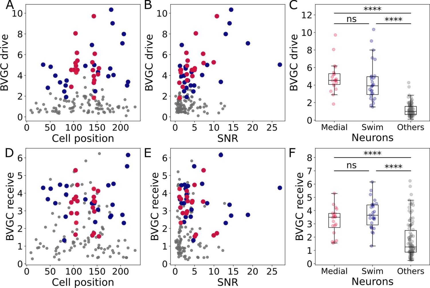
Correlation of the drive and receiving values with the cell position and signal-to-noise ratio, and comparison across neuron groups.
Correlation of the drive and receiving values with the cell position and signal-to-noise ratio, and comparison across neuron groups. (A) The neuronal drive, calculated as the sum of the strength of all outgoing Granger causality (GC) links for each neuron, is not correlated to the neuron position. In data recorded by a two-photon laser scanning microscope, different pixels are scanned across the sample with a very small delay. Panel A shows that the scanning direction and delay do not influence the GC results. (B) The neuronal drive is correlated to the signal-to-noise ratio (SNR) of the calcium traces. It is especially high for medial neurons (in red, compared to across all 139 neurons). After computing the new threshold for significance with a corrected null hypothesis and the normalized GC values, the correlation between the drive and SNR decreased. (C) The neuronal drive is significantly higher for motor-correlated neurons than for other neurons (Mann-Whitney U test; for not significant when , when ). This observation suggests that motor-correlated neurons are important drivers of the network activity. (D) The receiving value of a given neuron is defined as the sum of all its incoming GC links. As for the drive, it is not correlated to the cell position. (E) The receiving value is correlated to the SNR. This correlation is reduced when computing the receiving value using the normalized GC values. (F) The receiving value is significantly higher for motor-correlated than for other neurons. This shows strong information flow between the motor-correlated neurons (Mann-Whitney U test; when , when ).
Figure 8—figure supplement 2
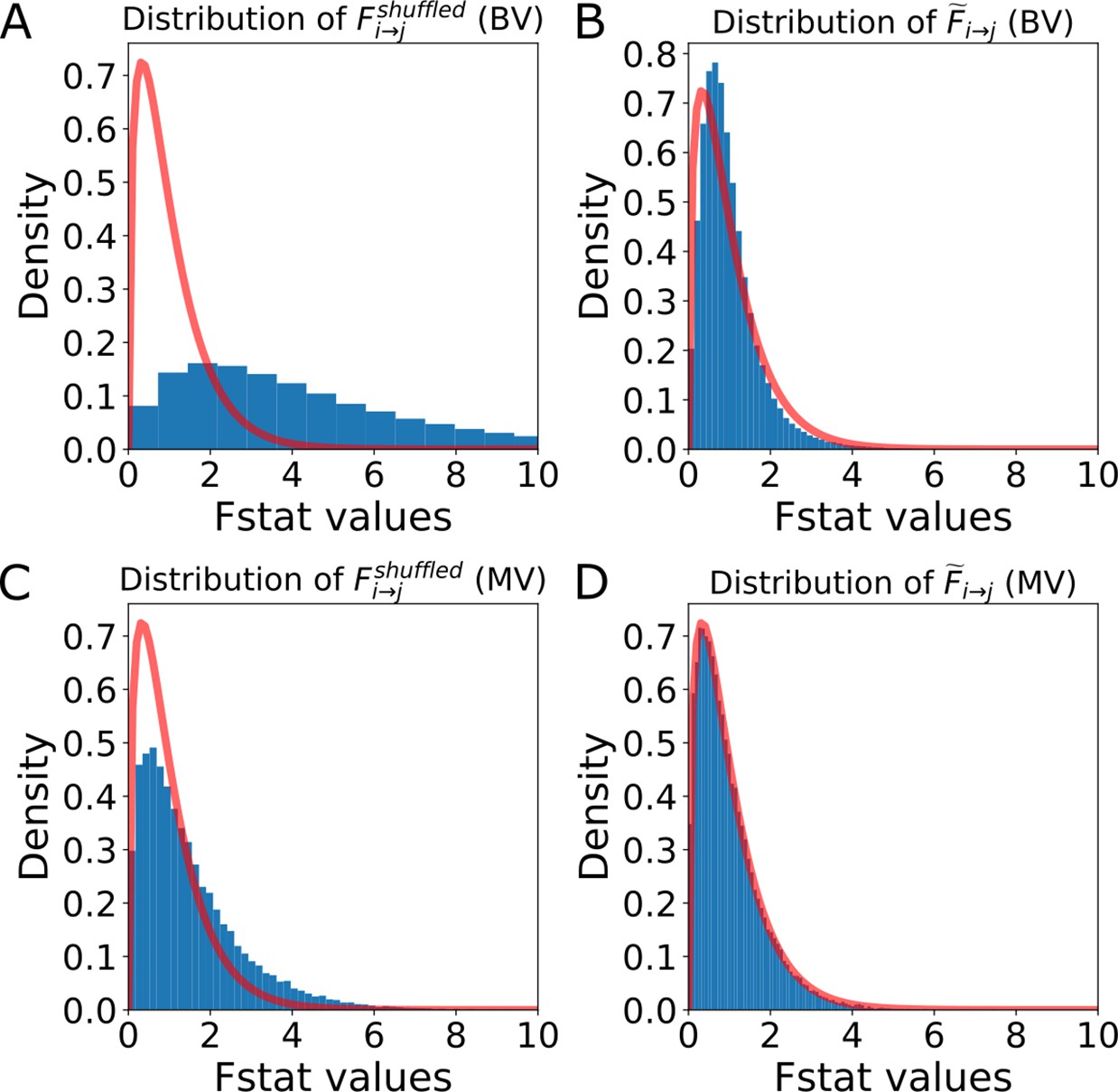
Distribution of the F-statistics of the shuffled data before and after re-scaling.
Distribution of the F-statistics of the shuffled data before and after re-scaling. (A) Original distribution of the BVGC F-statistics of shuffled data, . It has a shifted support that is larger than that of the F-distribution (red curve), meaning that if we use the original F-test based on the F-distribution as a null model, even if there are no Granger-causal links between two neurons, we will classify the link as significant. (B) For each neuron pair, the distribution is well-described by a constant-rescaled F-distribution. Applying an adaptive threshold on can be simplified to applying the original threshold on the normalized, defined by dividing the naive F-statistics with the expectation value of the F-statistics generated by the shuffled data (). (C) Original distribution of the MVGC . (D) The normalized is almost perfectly described by a constant-rescaled F-distribution.
Figure 8—figure supplement 3
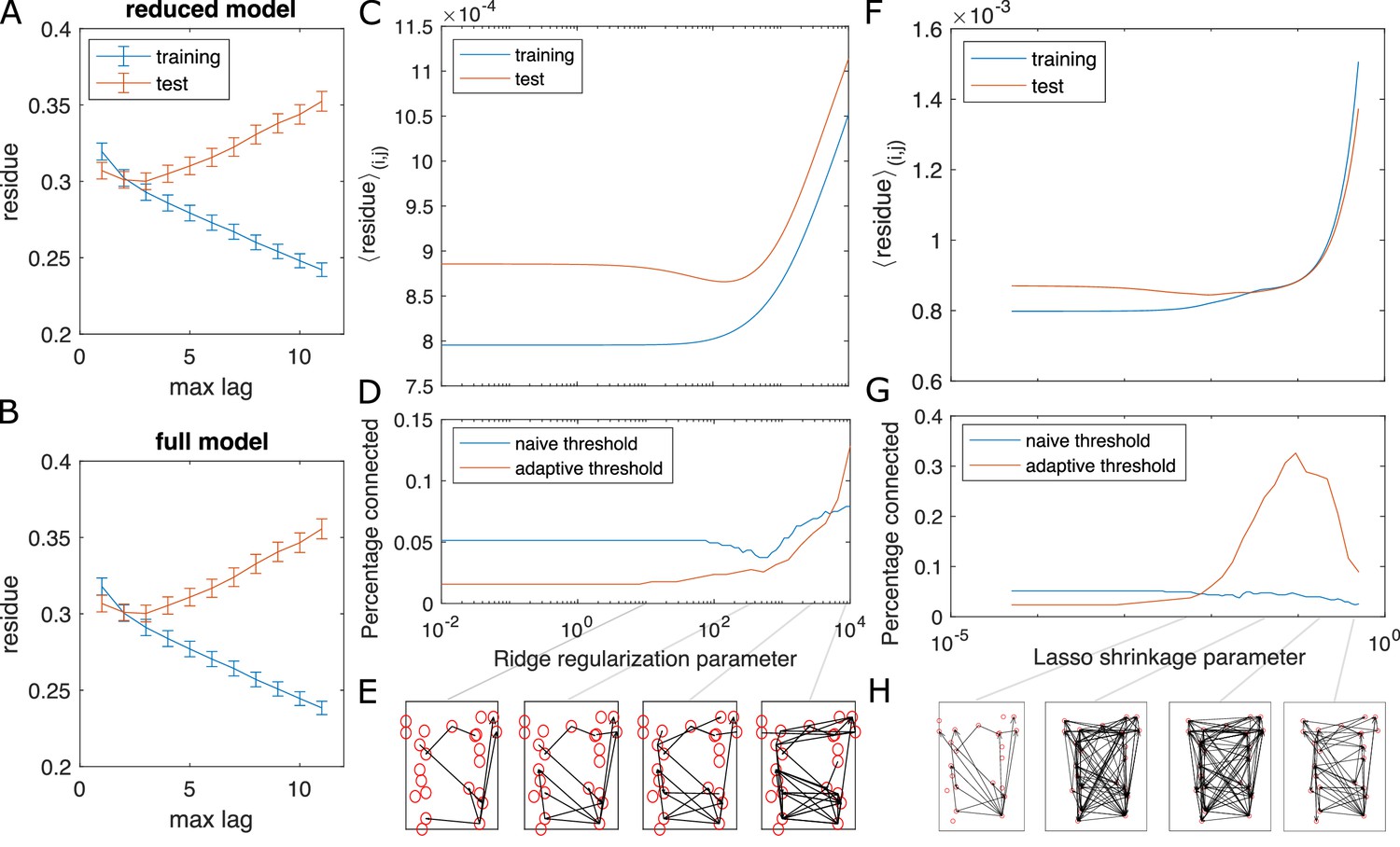
Test for overfitting and information flow from regularized GC on zebrafish hindbrain.
Test for overfitting and information flow from regularized GC on zebrafish hindbrain (N = 23 neurons). (A, B) Residues of the VAR model with different max lags for training (the first 2/3 of the data) and test (last 1/3 of the data) datasets, computed for and averaged across each possible neuron pair (i, j) for neuron j driving neuron i. The overlap between the training and test curves for max lag less than or equal to 3 shows the choice of max lag does not overfit. Error bars are standard error of the mean across all possible pairs of neurons. (C) The training and testing residue using ridge regularization for the full model shows a preferred ridge regularization parameter (D) The percentage of connection after GC analysis shows a decrease at the preferred ridge regularization parameter, if we use the naive threshold. Using adaptive threshold increases the connection. (E) Shows examples of information flow at different ridge regularization parameters, using the adaptive threshold. (F–H) Same as (C–E), using LASSO regularization.
Figure 8—figure supplement 4
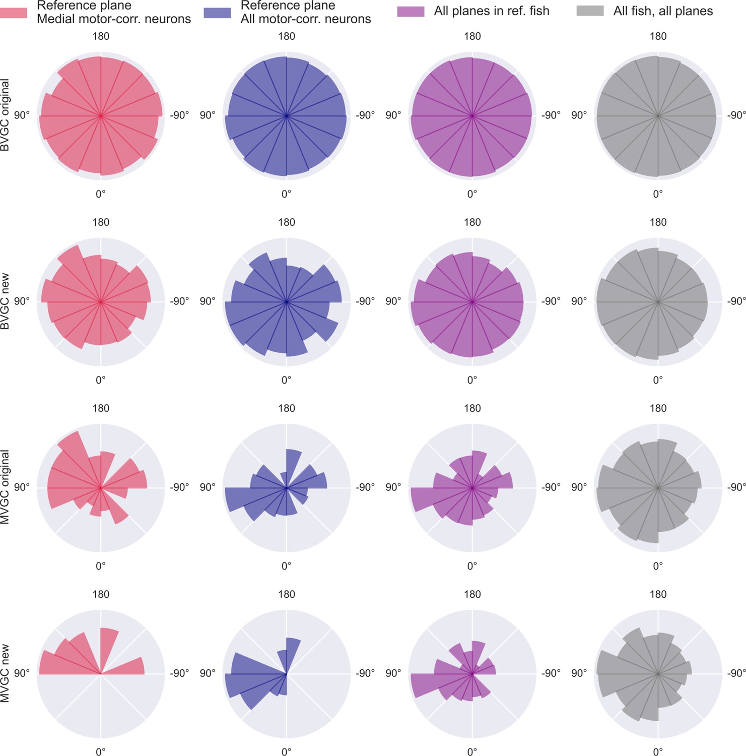
Distribution of GC link directions.
Distribution of GC link directions. Polar histogram of the proportion of angles of significant Granger causality links over all possible GC links between neurons. Using the naive bivariate GC (top row), we obtain a network that is almost fully connected, thus the proportion is close to 100% for all links and the polar histogram is close to a circle. The results of the adapted bivariate GC (2nd row), the naive multivariate GC (3rd row), and the adapted multivariate GC (bottom row), show a majority of links from right to left, suggesting an information flow from the right to the left hindbrain. This result is obtained in the medial swim-correlated neurons of the reference plane (N = 20 neurons, red, left column) and is conserved when GC is applied to all swim-correlated neurons of this plane (N = 41 neurons, blue, 2nd column), as well on swim-correlated neurons of all planes the reference fish (11 planes, 176 neurons in total, purple, third column), and across all swim-correlated neurons of all planes of all fish (n = 10 fish, 975 neurons in total, gray, right column).
Figure 8—figure supplement 5
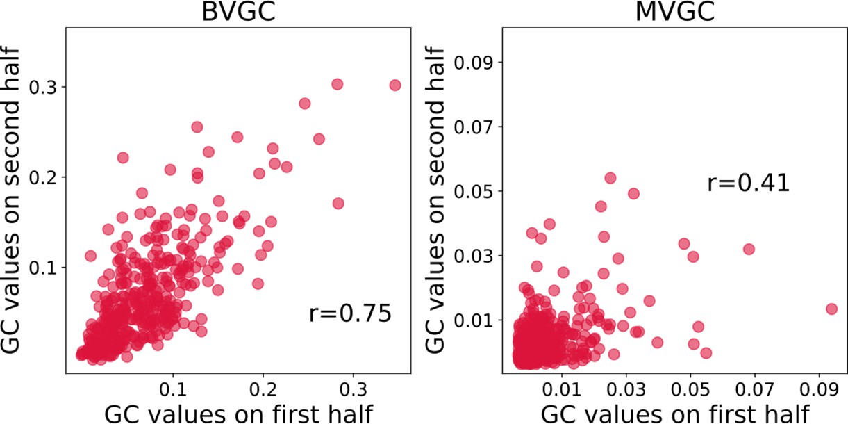
Correlation of Granger causality values using the first and second halves of the hindbrain data.
Correlation of Granger causality values using the first and second halves of the hindbrain data (N = 41 neurons). The correlation of for the two halves assesses that BVGC (left) can be applied to the whole time series (1744 time steps). The correlation between the MVGC analyses of the halves of the hindbrain dataset (right) is low, and in this case, 872 time points are not sufficient to infer reliable MVGC results.
Figure 9
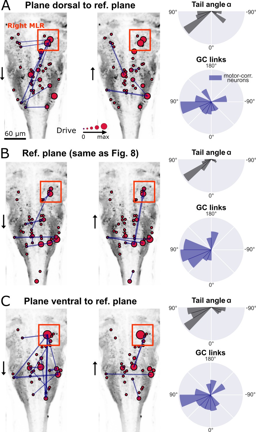
New multivariate Granger causality analysis of motor-correlated hindbrain neurons revealed neurons in the locus of Mesencephalic Locomotor Region (MLR) on the side of the visual grading driving activity of neurons in the contralateral MLR and on both sides in the medulla.
The distributions of the tail angles for turns (tail angle with , gray, top left of A-C) and the distributions of the new MVGC link angles (blue, bottom left of A-C) indicate a bias when the visual grading stimulus was presented on the right towards the left across 3 hindbrain planes spaced by 10µm (A: plane 5, dorsal to B: plane 7, analyzed in Figure 8; C: plane 9, ventral to plane 7). Across these three planes, a group of strong driver neurons (middle and right panels of A-C) was found located on the right, in the locus of the MLR. This is to our knowledge the first evidence of recruitment of cells in the MLR locus during locomotion. As expected from anatomy (Carbo-Tano et al., 2022), right MLR neurons drive contralateral neurons in the left MLR and in the medulla where the reticular formation is located, both on the right and left sides.
Tables
Table 1
The directional measures for the bivariate and multivariate GC network for the calcium transients f3t1 before and after motion-artifact correction, a pre-processing step for calcium signals.
The GC network after motion artifact correction has clear ipsilateral structures.
| BVGC | MVGC | |||
|---|---|---|---|---|
| Before MA correction | 0.39 | 0.53 | 0.43 | 0.52 |
| After MA correction | 0.66 | 0.56 | 0.68 | 0.44 |
Table 2
The directional measures for the bivariate and multivariate GC network for the calcium transients f5t2 before and after removal of the atypical neurons.
| BVGC | MVGC | |||
|---|---|---|---|---|
| With strange neurons | 0.56 | 0.51 | 0.59 | 0.38 |
| Without strange neurons | 0.54 | 0.67 | 0.53 | 0.53 |
Additional files
Download links
A two-part list of links to download the article, or parts of the article, in various formats.
Downloads (link to download the article as PDF)
Open citations (links to open the citations from this article in various online reference manager services)
Cite this article (links to download the citations from this article in formats compatible with various reference manager tools)
Granger causality analysis for calcium transients in neuronal networks, challenges and improvements
eLife 12:e81279.
https://doi.org/10.7554/eLife.81279


