Beta oscillations and waves in motor cortex can be accounted for by the interplay of spatially structured connectivity and fluctuating inputs
- Laboratoire de Physique de l’Ecole Normale Supérieure, CNRS, Ecole Normale Supérieure, PSL University, Sorbonne Université, Université de Paris, France
- School of Physics and Electronic Science, East China Normal University, China
- Institut de Biologie de l’Ecole Normale Supérieure (IBENS), CNRS, Ecole Normale Supérieure, PSL University, France
Figures
Figure 1 with 4 supplements
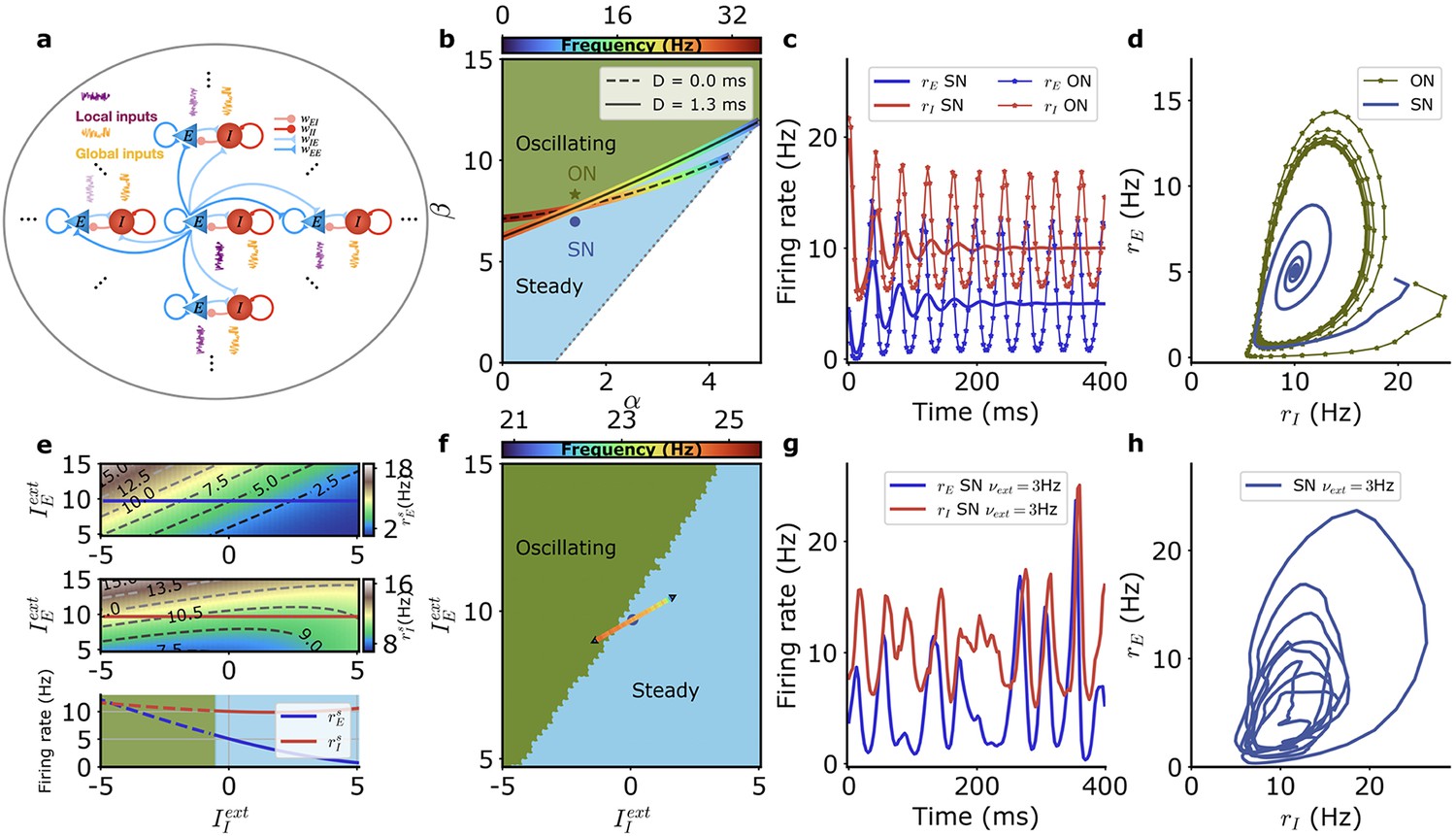
Model of neural network generating beta oscillations.
(a) Schematic depiction of the model with excitatory populations (blue), inhibitory populations (red), independent external inputs on each module (‘local,’ purple), and inputs common to all modules (‘global,’ orange). (b) Different dynamical regimes for fixed firing rates of the excitatory and inhibitory populations ( Hz, Hz), as a function of the strengths of recurrent excitation (α) and of feedback inhibition through the E-I loop (β) for a fixed value of recurrent inhibition in the inhibitory population , with the parameters and as defined in Equation 34. The oscillatory instability line for ms (solid black) and ms (dashed black) and the line of ‘real instability’ (short-dashed black) are shown. Color around the oscillatory lines indicates the frequency of oscillation along the bifurcation line. (c) Time series of the firing rate for the E (blue) and I (red) module populations at the SN (thick lines) and at the ON (thin lines with symbols) points. E and I population activities become steady at the SN point and display regular oscillations at the ON point. (d) Same data as in (c) for SN (blue) and ON (green) parameters but with plotted as a function of . (e) Firing rates of the E (top) and I (middle) populations for SN parameters when the external inputs are varied and (bottom) along the solid lines in top and middle panels when only the external input on the inhibitory population is varied (E blue, I red). The dashed parts of the line correspond to unstable steady states. (f) Different dynamical regimes as a function of the mean strength of external inputs for SN. The external inputs on each population vary along the colored line when the strength of the external input fluctuates. The color indicates the frequency associated with the linear dynamics at the respective stationary states. (g) Example of E and I activity time traces when the external inputs vary in time along the colored line in (f). (h) Same data as in (g) but with plotted as a function of . Model parameters correspond to SN and ON in Table 1.
Figure 1—figure supplement 1
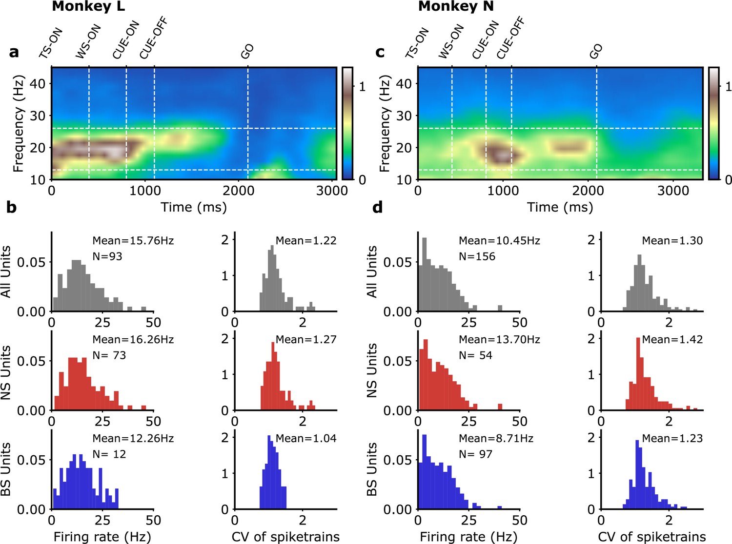
Recording data: LFP and single-unit characteristics.
(a, b) Monkey L, (c, d) monkey N. (a, c) Example spectrograms for individual trials of the experiments of Denker et al., 2018; Brochier et al., 2018. We focus here on the data between CUE-OFF and GO, the movement ‘preparatory period.’ (b, d) Characteristics of the single units spike sorted in Brochier et al., 2018 (monkey L, 93 units; monkey N, 156 units). Following Dąbrowska et al., 2021, spikes of width smaller than 0.4 ms were classified as narrow spike units (NS)/putative interneurons (monkey L, 73 units; monkey N, 54 units) and spike of width larger than 0.41 ms were classified as broad spike units (BS)/putative pyramidal cells (monkey L, 12 units; monkey N, 97 units) (units with spike width between 0.40 and 0.41ms are not classified).
Figure 1—figure supplement 2
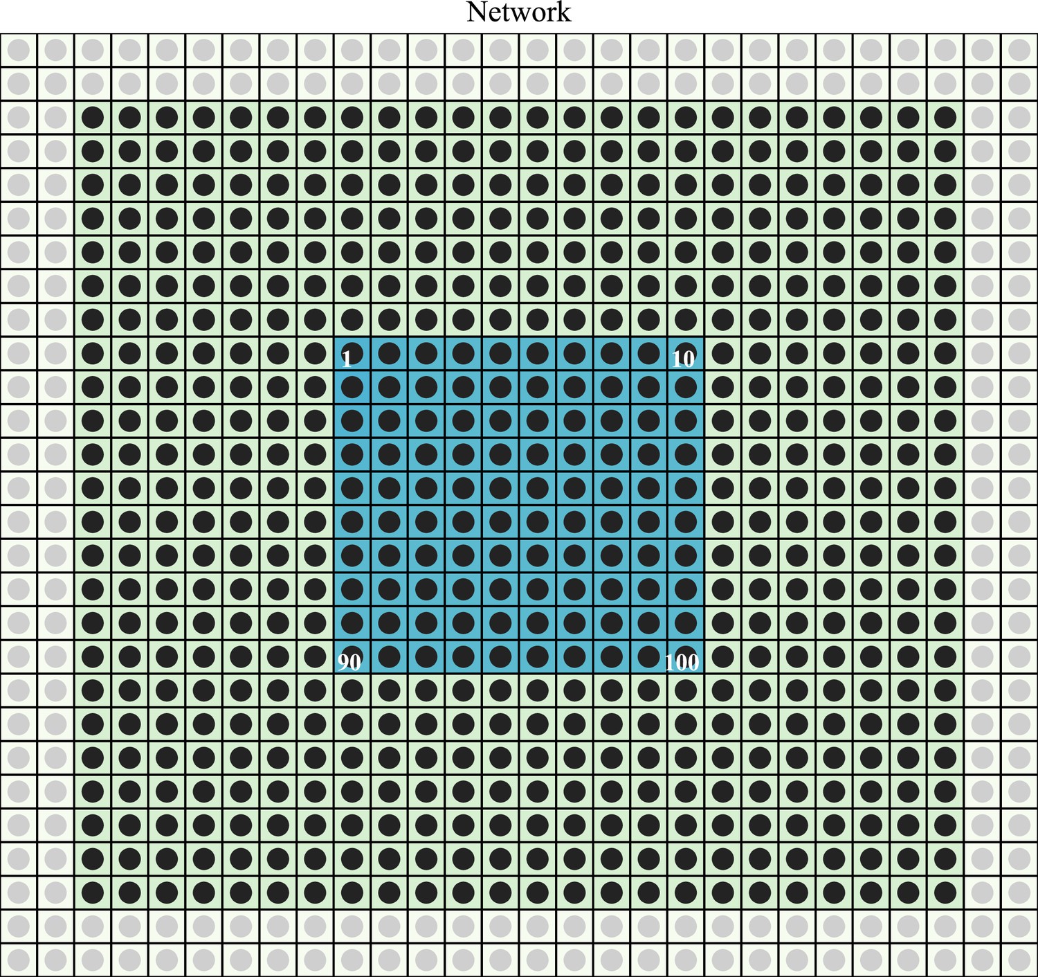
Numerical simulation grid.
Different E-I modules (disks) are placed at the center of the different squares. The discharge rates of the E-I populations in the two most external layers (gray disks) are fixed at their steady state values. The other modules (black disks) in the 24 × 24 central array are simulated. Only the modules in the 10 ×central array (blue squares) are used for the different signal measurements.
Figure 1—figure supplement 3
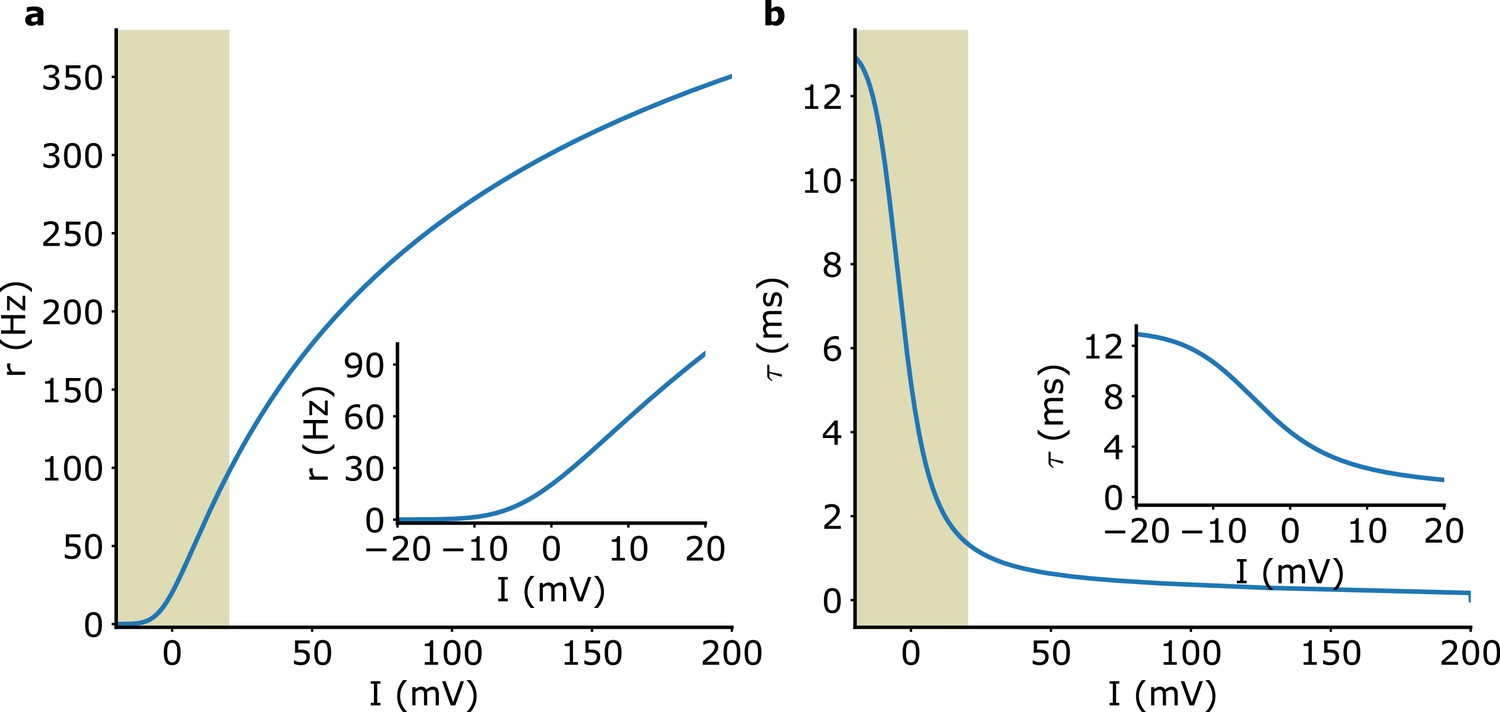
Rate model f-I curve and adaptive time scale.
(a) f-I curve. Inset: zoom on the 0−100 Hz region. (b) Adaptive time scale. The data corresponding to these curves are provided with our simulation code at https://github.com/LKANG777/Beta-Oscillation (copy archived at Kang, 2023).
Figure 1—figure supplement 4
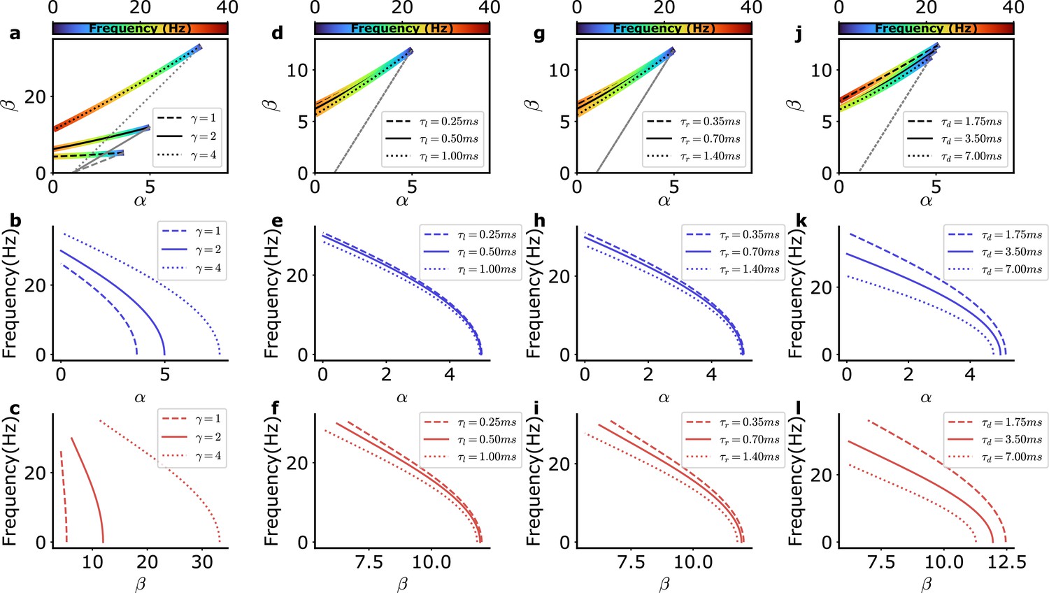
Dependence of the bifurcation lines and frequency on model parameters.
(a–c) Dependence on recurrent inhibition between interneurons as measured by the parameter (Equation 34), (d–l) dependence on synaptic current kinetics: (d–f) latency , (g–i) rise time , and (j–l) decay time . Top: Bifurcation lines as in Figure 1b but for varying (a) or synaptic kinetics (d, g, j). Center, bottom: frequency dependence on the bifurcation lines (top) as a function of the recurrent excitation among excitatory neurons () (center; b, e, h, k) or the strength of recurrent inhibition through the E-I loop () (bottom; c, f, i, l).
Figure 2 with 3 supplements
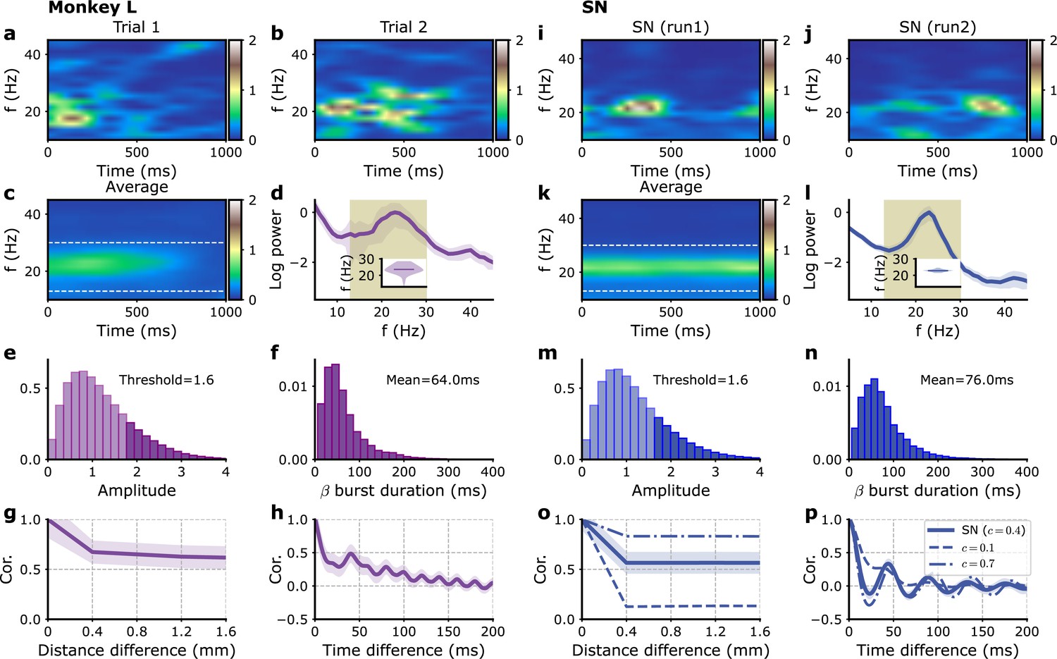
Single-electrode recordings vs. model E-I module dynamics with fluctuating inputs.
(a–h) Monkey L recordings (Brochier et al., 2018), (i–p) model simulations. (a, b) Two examples of single trial spectrograms of a single-electrode LFP during the preparatory period (the CUE-OFF to GO period in Figure 1—figure supplement 1). (c) Spectrogram averaged over different trials and different electrodes. (d) Power spectrum of single-electrode LFP averaged over all electrodes. Average over trials (solid violet line) and standard deviation of fluctuation over trials (violet shaded region). Inset: violin plot showing the distribution over trials of the average power spectrum peak frequency in the 13–30 Hz interval. (e) Distribution of beta oscillation amplitudes. The amplitude of oscillation corresponding to the beta burst are shown in darker color. (f) Distribution of beta burst duration. (g) Average LFP cross-correlation between two electrodes as a function of their distance. (h) Auto-correlation of single LFP time-series averaged over trials and electrodes. (i–p) Corresponding panels for simulations with model SN. (i, j) Two examples of single modules spectrograms of 1 s time series. (k) Average time series spectrogram. (i) Corresponding power spectrum (see d for a detailed description). (o) Cross-correlations between different modules times series as a function of their distance, for different fractions of global (i.e., shared) external inputs, (solid), (dashed), and (dashed-dotted). (p) Auto-correlation of single module time series for the different fractions in (o). Model parameters correspond to SN in Table 1.
Figure 2—figure supplement 1
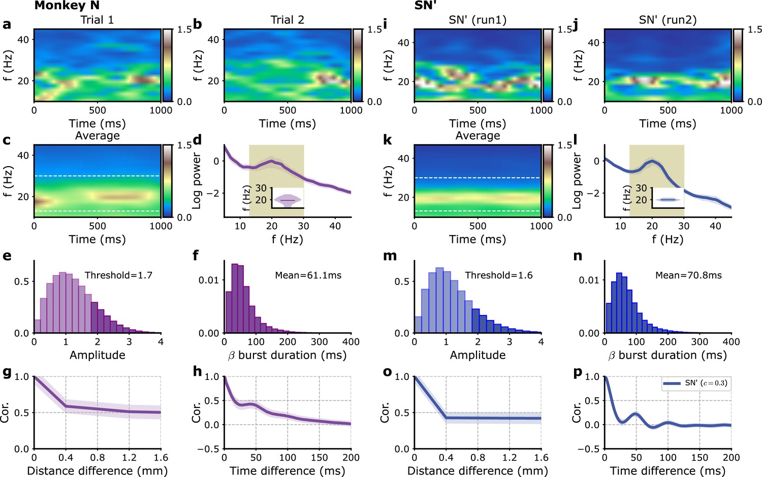
Beta bursts and power spectra for monkey N.
Figure 2—figure supplement 2
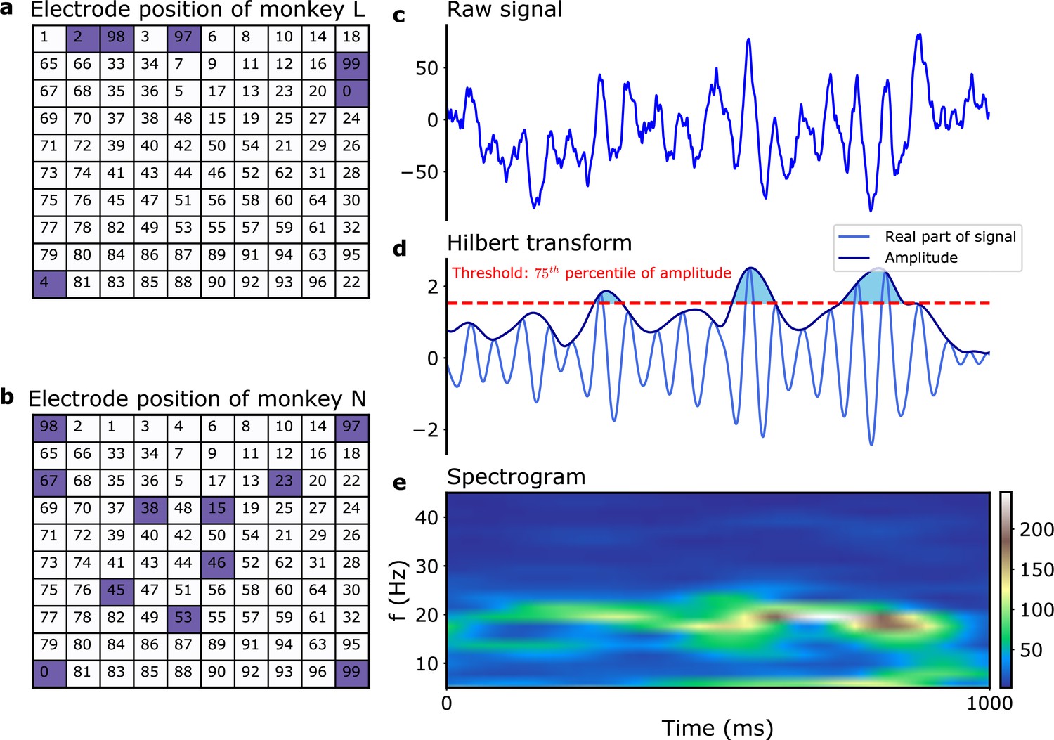
Data analysis: filtering and burst amplitude threshold.
Electrode positions and numbering in Brochier et al., 2018 for (a) monkey L and (b) monkey N. The blue squares indicates the positions of the dead electrodes. (c–e) Illustration of data analysis. (c) 1 s of single-electrode signal (monkey N, electrode 7, trial 1). (d) Same signal after bandpass filtering. The amplitude threshold used to define the beta bursts is indicated (dashed red line). The corresponding beta bursts themselves correspond to the shaded blue regions. (e) Spectrogram of the signal in (c).
Figure 2—figure supplement 3
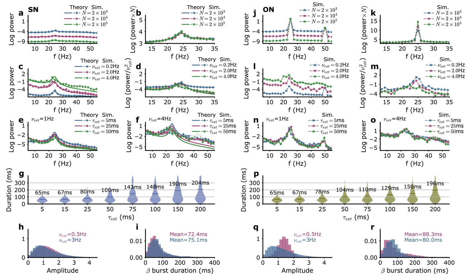
Model power spectra and beta bursts as a function of the external input parameters.
(a–i) SN parameters, (j–r) ON parameters. (a, j) Power spectra for different numbers of neurons in each module corresponding to different levels of intrinsic noise without fluctuations of external inputs. For the SN parameters, the analytical formula Equation 51 is also shown (solid lines). (b, k) Power spectra multiplied by the number of neurons . In this range of amplitude, the power spectra have the same shape when normalized by the amplitude of the stochastic fluctuations. (c, l) Influence on the power spectra of the amplitude of external input fluctuations. (d, m) Power spectra divided by . (e, f, n, o) Influence on the power spectra of the correlation time for two amplitudes of external input fluctuations. (g, p) Influence on the beta burst duration of the correlation time of external input fluctuations. Distribution of beta burst amplitudes (h, q) and durations (i, r) for two amplitudes of external input fluctuations. Parameters of the input that are not explicitly varied as well as the network parameters for models SN and ON are given in Table 1.
Figure 3 with 12 supplements
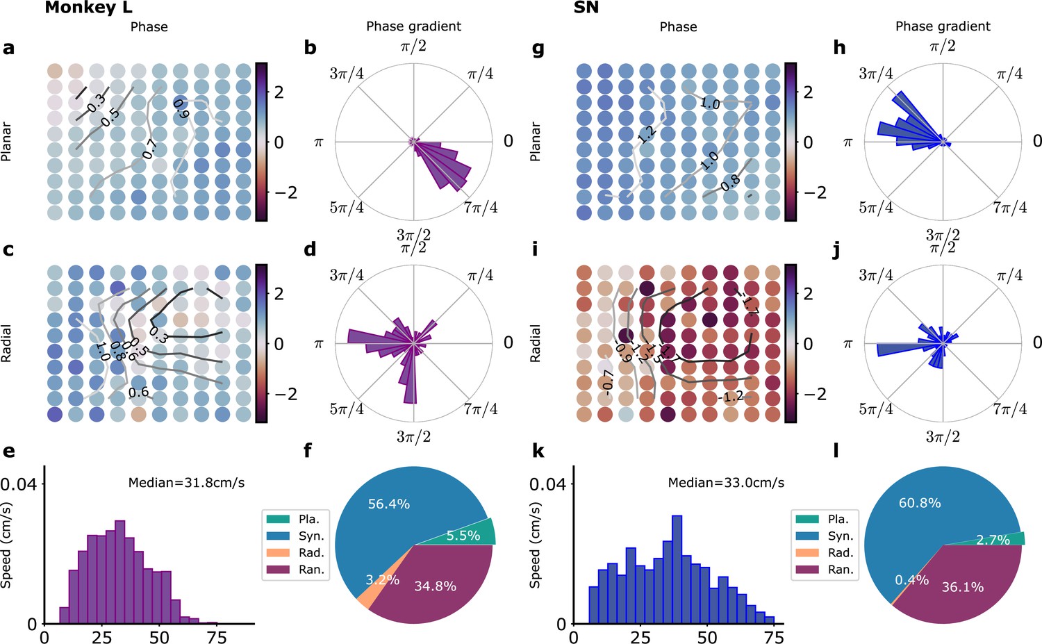
Waves in recordings and in model simulations.
(a–f) Monkey L recordings (Brochier et al., 2018), (g–l) Model simulations with SN parameters. (a) Snapshot of a planar wave. The phases of the LFP on the different electrodes are shown in color. Smoothed phase isolines are also shown (thin lines). (b) Distribution of phase gradients on the multielectrode array in (a). Note the high coherence of the phase gradients (). (c) Example of a radial wave with LFP phases and isolines displayed as in (a). (d) Corresponding distribution of phase gradients (). (e) Distribution over time and trials of measured planar wave speeds. (f) Proportion over time and trials of planar (Pla.), synchronous (Syn.), radial (Rad.), and random (Ran.) wave types. (g–l) Corresponding model simulations. (g) Snapshot of a planar wave showing the phases of different modules. (h) Distribution of phase gradients () in (g). (i) Snapshot of a radial wave. (j) Distribution of phase gradients in (i) (). (k) Distribution of planar wave speeds. (l) Proportions of different wave types.
Figure 3—figure supplement 1
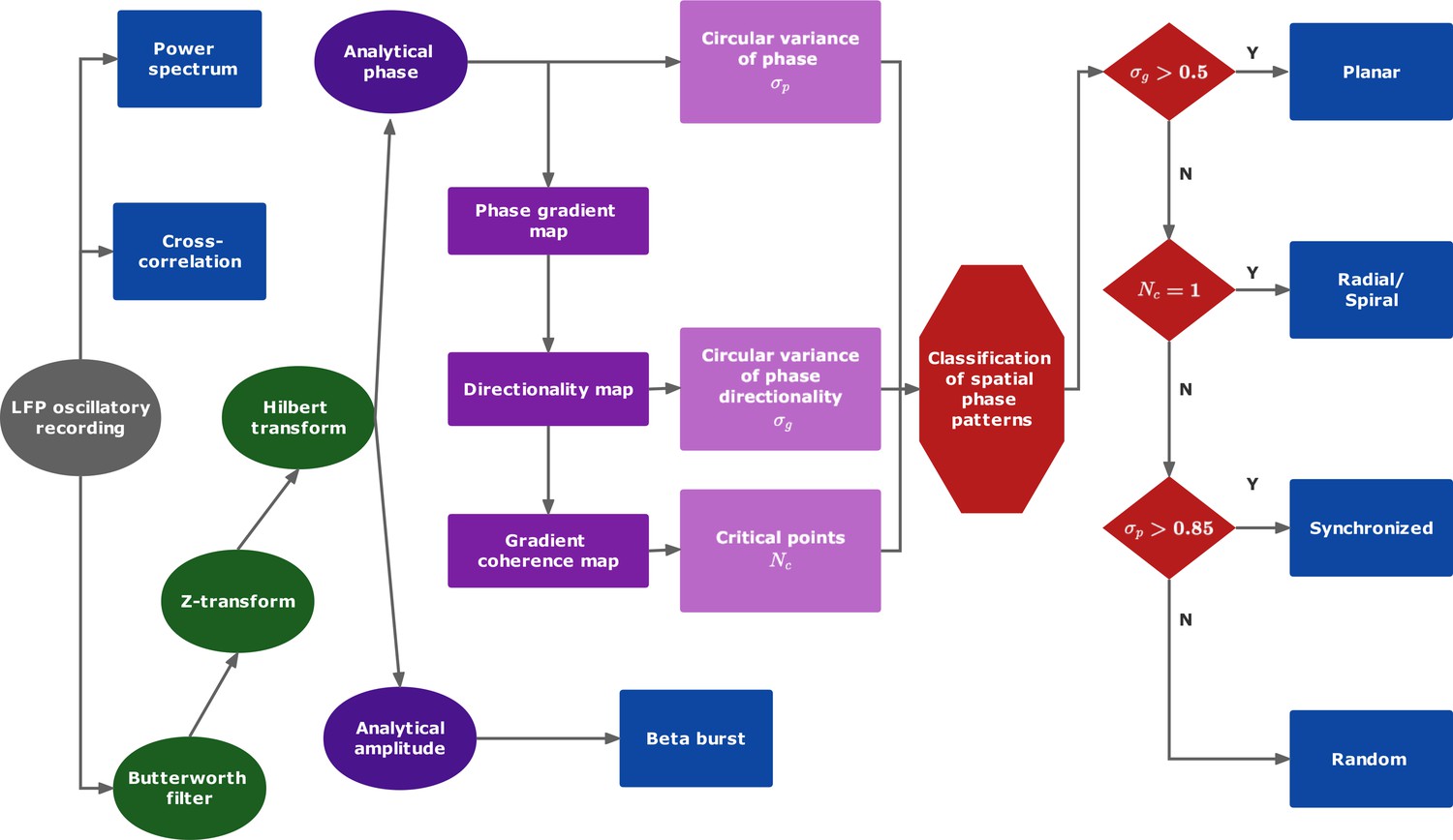
Data analysis protocol.
See ‘Methods for a description of the different steps.
Figure 3—figure supplement 2
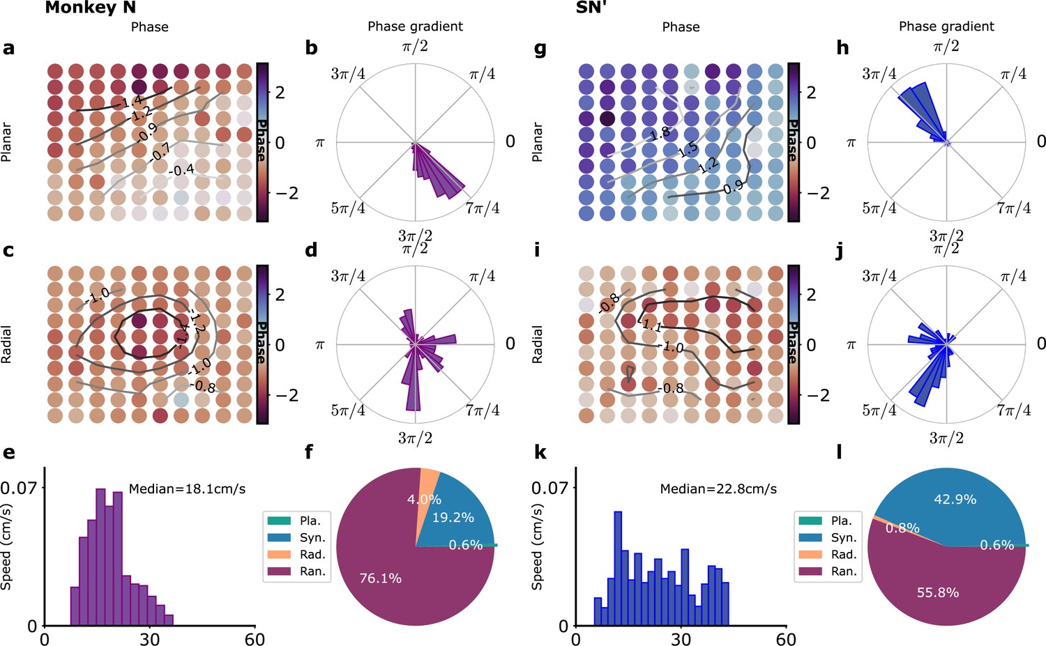
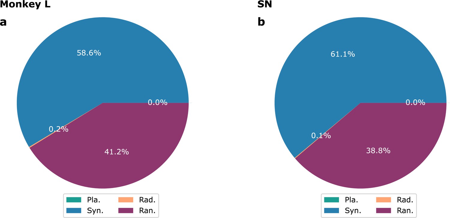
Waves in model simulations and in recordings for monkey N.
Figure 3—figure supplement 3
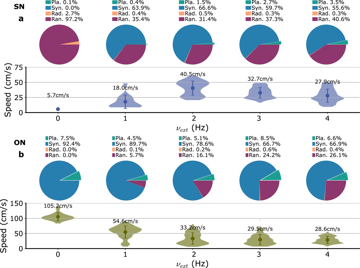
Variation of wave type distribution and planar wave speed with the amplitude of the external input fluctuations ().
(a) SN parameters. (b) ON parameters.
Figure 3—figure supplement 4
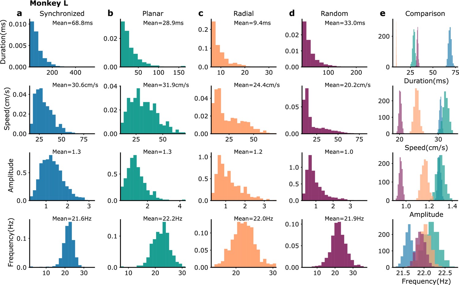
Waves statistics in monkey L recordings.
(a–e) Distributions over different wave events of their duration, mean speed, mean amplitude and mean frequency for (a) synchronized (blue), (b) planar (green), (c) radial (orange), and (d) random (violet) events. (e) Distributions of the average duration, mean speed, mean amplitude, and mean duration (averaged over events) obtained by bootstrap sampling (3000 repetitions with the number of events in each sample equal to the number of events in the corresponding wave type category [Syn: 1223, Pla: 286, Rad: 510, Ran: 1834]). The colors correspond to the ones of the respective wave types in (a–d).
Figure 3—figure supplement 5
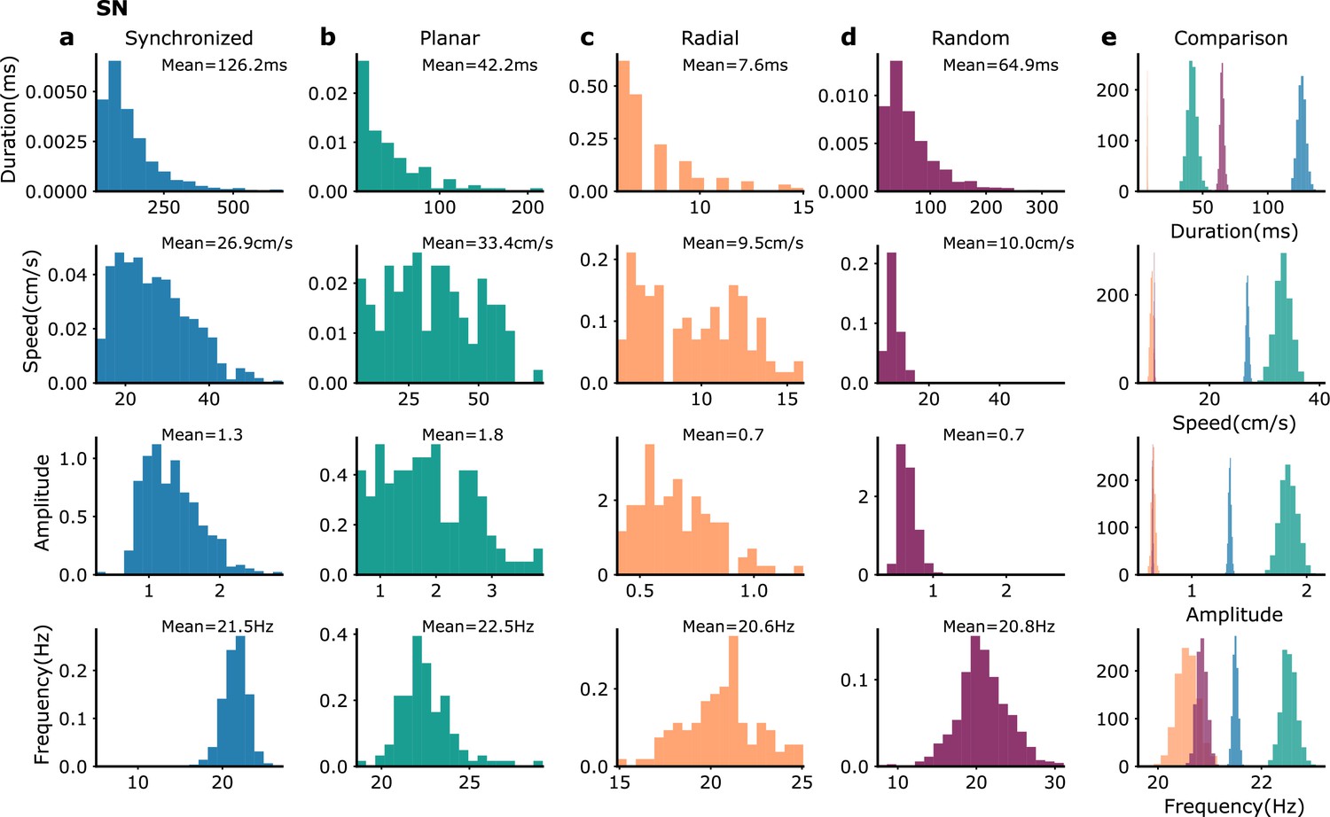
Waves statistics in SN model simulations.
Same as Figure 3—figure supplement 4 but for waves in SN model simulations. The numbers of wave events in the different categories are (Syn: 992, Pla: 115, Rad: 105, Ran: 1056).
Figure 3—figure supplement 6
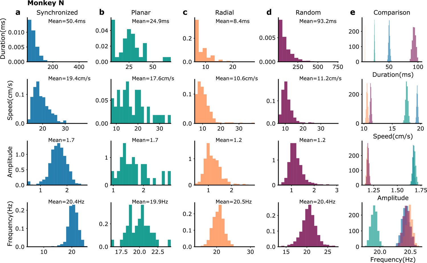
Waves statistics in monkey N recordings.
Same as Figure 3—figure supplement 4 but for waves in monkey N recordings. The numbers of wave events in the different categories are (Syn: 597, Pla: 40, Rad: 749, Ran: 1272).
Figure 3—figure supplement 7
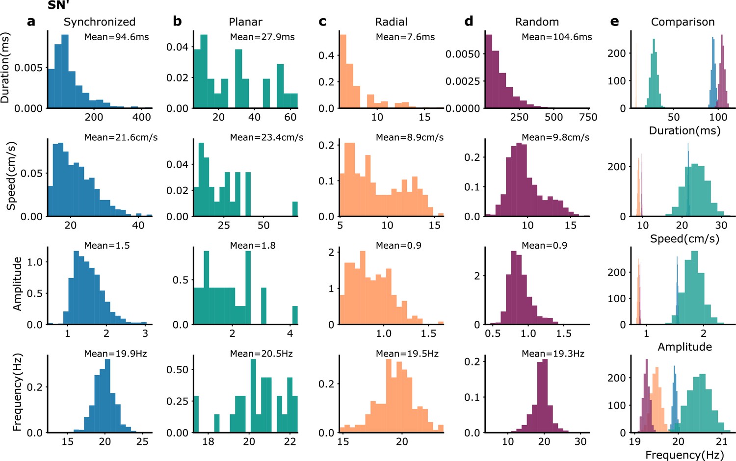
Waves statistics in SN’ model simulations.
Same as Figure 3—figure supplement 4 but for waves in SN’ model simulations. The numbers of wave events in the different categories are (Syn: 964, Pla: 27, Rad: 211, Ran: 1175).
Figure 3—figure supplement 8
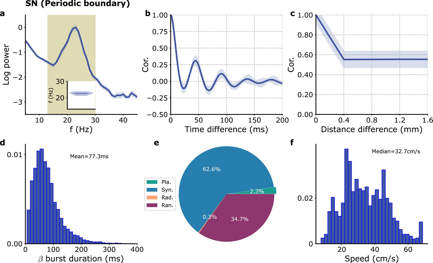
Simulation of the model of Figure 3 with periodic boundary conditions.
Simulation grid size 24 × 24 with all signals recorded in a 10 × 10 grid as in Figure 3.
Figure 3—figure supplement 9
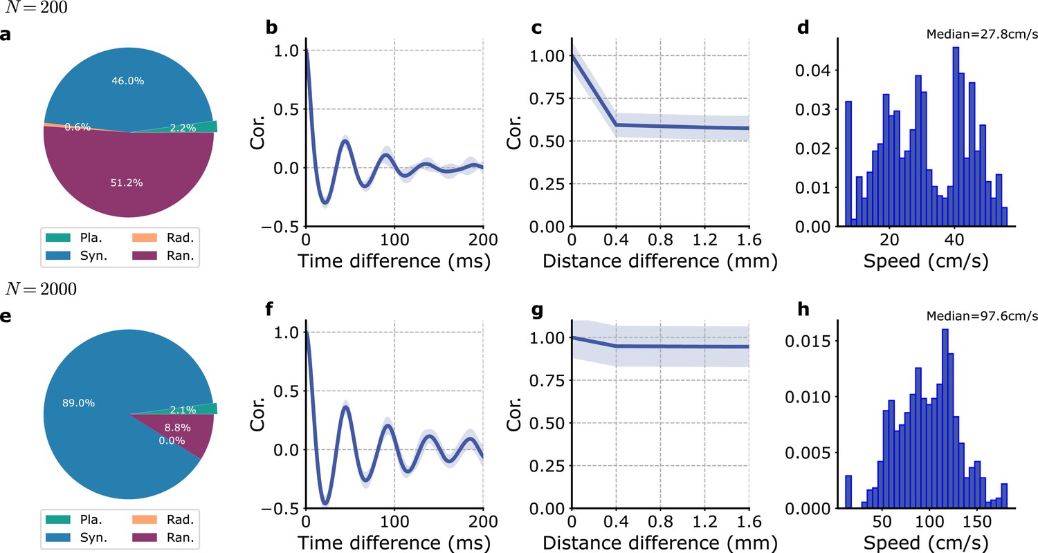
Intrinsic stochasticity without local inputs.
(a–d) N = 200, (e–h) N = 2000. (a, e) Proportions of the different wave types. (b, f) Auto-correlation in time of the module proxy-LFP (). (c, g) Cross-correlations between different modules proxy-LFP vs. module distance. (d, h) Distribution of observed planar speeds.
Figure 3—figure supplement 10
Proportion of different waves for shuffled signals.
(a) Monkey L recordings; (b) model of Figure 3. See the main text for description.
Figure 3—figure supplement 11
Model with no propagation delay.
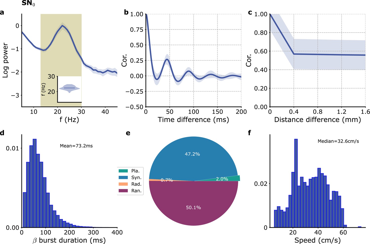
(a) Single module power spectrum. (b) Single module auto-correlation. (c) cross-correlation as a function of module distance. (d) Distribution of beta burst duration. (e) Proportion of different wave types. (f) Distribution of speeds of planar waves. Model parameters correspond to SN0 in Table 1.
Figure 3—figure supplement 12
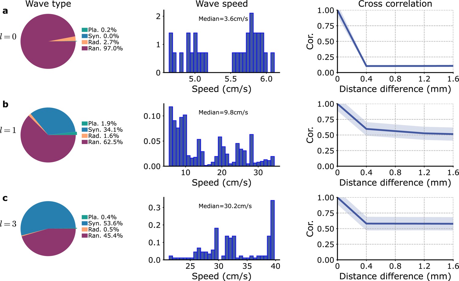
Variation of the excitatory connectivity range, , in the model of Figure 3—figure supplement 11.
The proportions of the different wave types (left), the wave speed distributions for planar waves (center), and the cross-correlation of between modules as a function of their distance (right) are shown for different : (a) , (b) , and (c) .
Figure 4 with 2 supplements
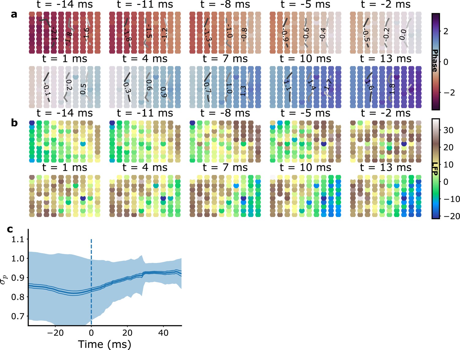
Average planar wave characteristics and the role of global inputs.
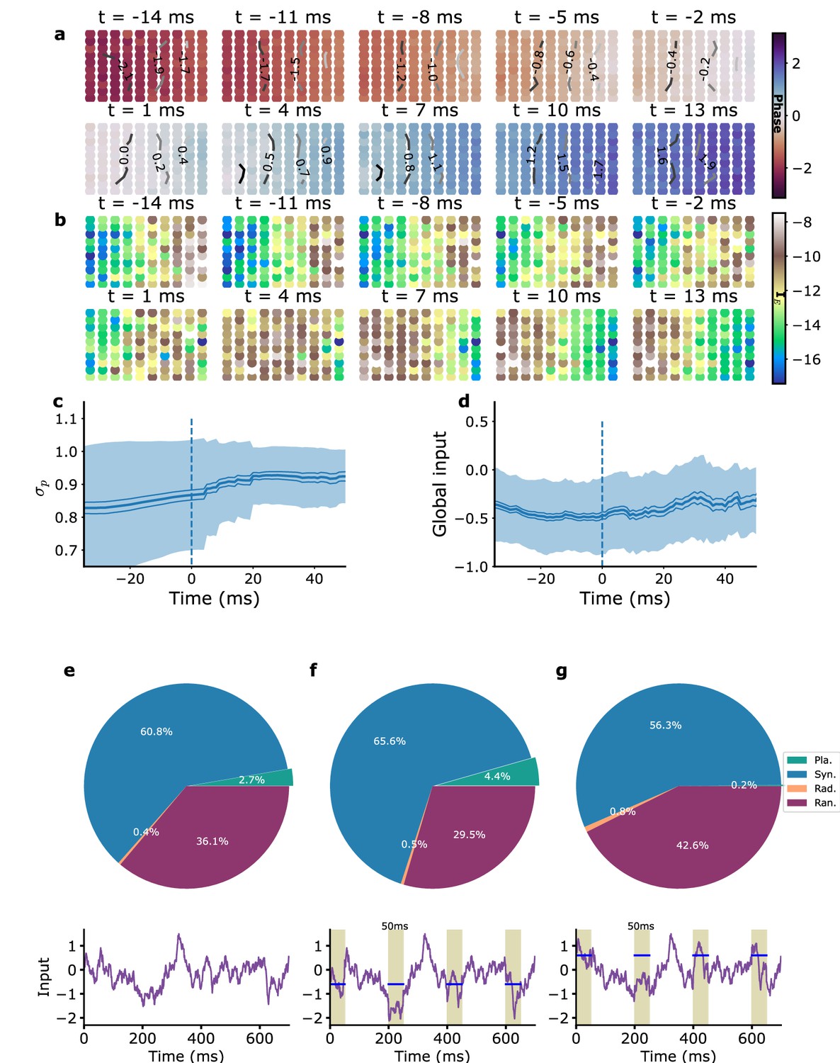
(a) Average phase, (b) average excitatory current (proxy-LFP), (c) average synchronization parameter , and (d) average global external input. For (a, b), planar waves were aligned in time by matching their average phases around mid-event, and rotated to make wave directions coincide (see ‘Methods’). The time corresponds to zero average phase. For (c, d), planar waves were aligned in time based on wave onset (vertical dashed blue line), corresponding to time in these panels. (e–g) Stimulation by global currents modifies planar wave proportion (top). Typical traces of the global inputs including the fluctuating part and the additionally injected current for the three cases are shown in the graphs below (purple lines); periods of injection are shown as shaded areas and injection strength is indicated by the blue bars. (e) Without additional stimulation, the mean number of planar wave events per simulation is with a mean duration of each event ms ( simulations of 10 s each). (f, g) Wave proportions with injected current. (f) Negative stimulation with an amplitude comparable to that observed in (d) produces a greater number of planar wave events (, one-tailed Welch’s t-test), mean duration of planar wave events ms. (g) Positive stimulation decreases the number of planar waves events , (, one-tailed Welch’s t-test), mean duration of planar wave events ms. The proportion of the different wave types is shown in the three cases.
Figure 4—figure supplement 1
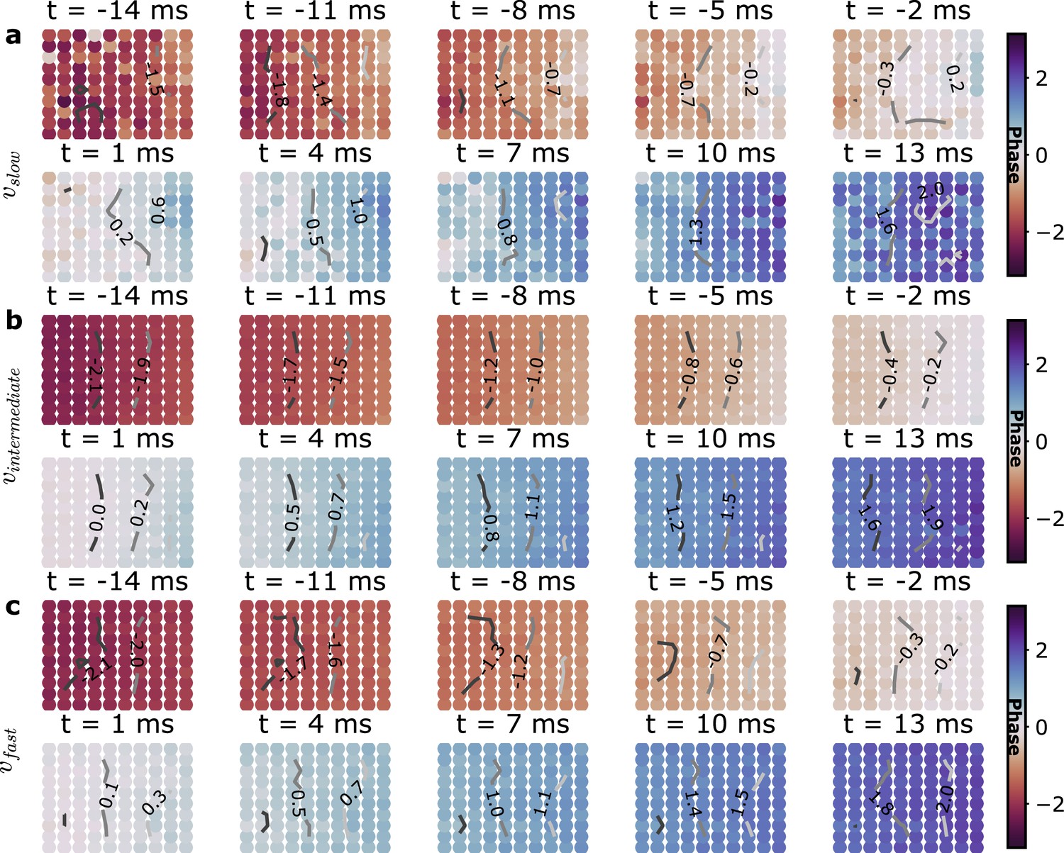
Average planar wave spatio-temporal phase maps.
Same as Figure 4a but with the planar wave episodes separated in three speed groups: (a) slow (lt25 cm/s), (b) intermediate (25−45 cm/s), and (c) fast (gt45 cm/s).
Figure 4—figure supplement 2
Average spatio-temporal planar wave maps for monkey L recordings.
(a) Phase maps, (b) LFP maps, and (c) average . Analogous to Figure 4a–c for the model SN.
Figure 5 with 1 supplement
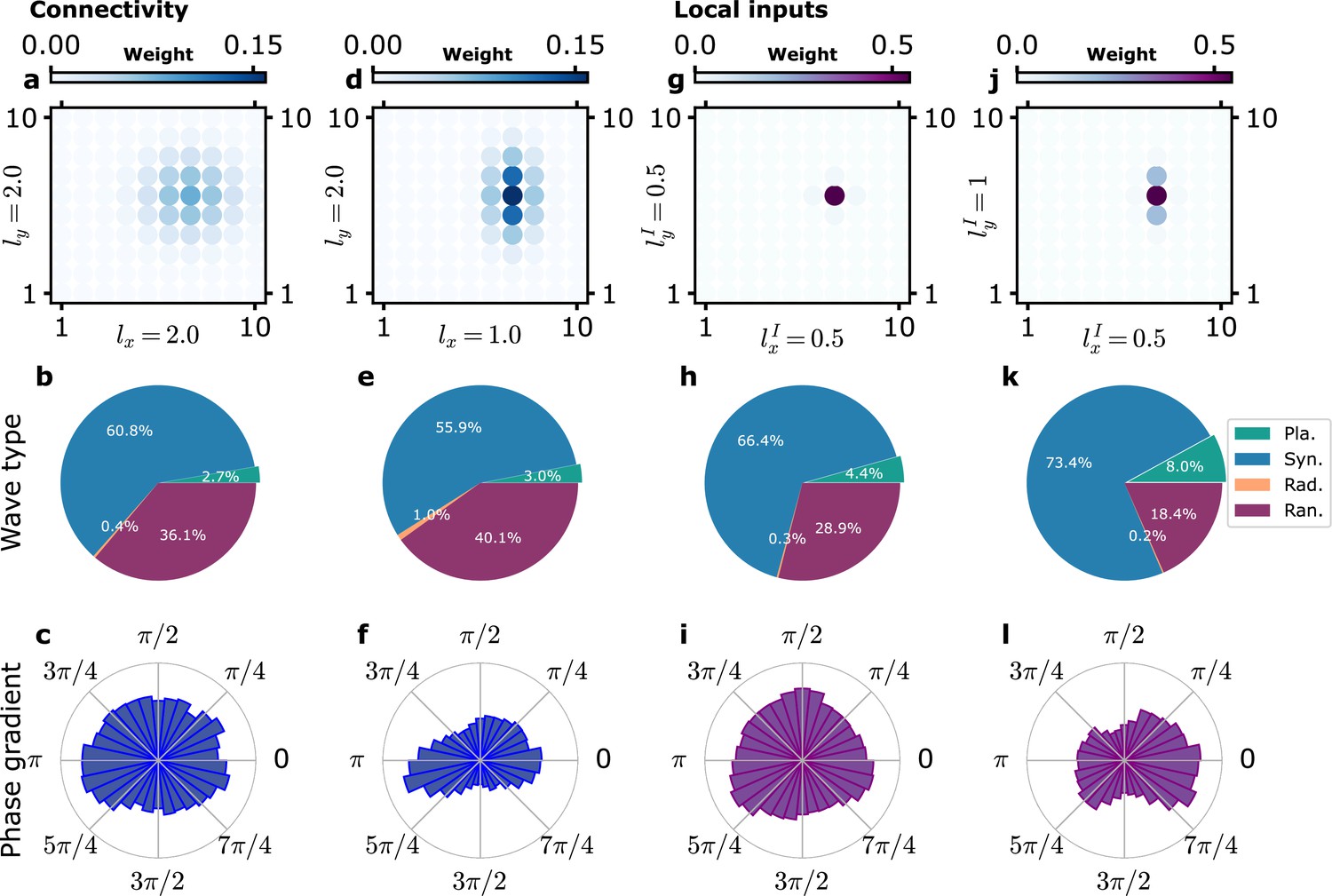
Influence of anisotropy of connectivity or local inputs on planar wave propagation direction.
(a–f) Effect of anisotropic recurrent connectivity. (a–c) Model simulations with an isotropic connectivity as in the previous figures. (d–f) Model simulations with an anisotropic connectivity. (a, d) The function is shown (with arbitrarily chosen at position (7,6)). (b, e) Proportion of different wave types. (c, f) Distribution of propagation directions of planar waves. In (f), the planar waves predominantly propagate along the x-axis, the axis along which decreases the fastest. (g–l) Effect of anisotropy of local inputs. (g–i) Model simulations with isotropic local inputs. This is similar to previous figures with the difference that local inputs targets adjacent modules weighted by a Gaussian kernel (Equation 22). (j–l) Model simulations with anisotropic local inputs. (g, j) The function is shown (with arbitrarily chosen at position (7,6)). (h, k) Proportion of different wave types. (i,l) Distribution of propagation directions of planar waves. In (l), the planar waves predominantly propagate along the x-axis, the axis along which decreases the fastest.
Figure 5—figure supplement 1
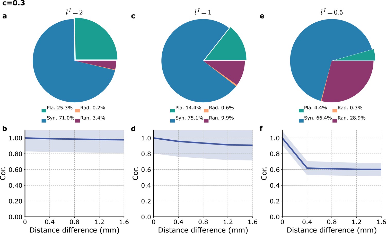
Model with a generalized description of local inputs.
Simulations of the model where the targets of local inputs are weighted by a Gaussian kernel function of range in grid units (Equation 22, see main text and ‘Methods’). (a, b) , (c, d) , and (e, f) . (a, c, e) Proportion of different wave types. (b, d, f) Cross-correlation of the proxy-LFP () as a function of the distance between different modules. The results in (e, f) are similar to those obtained in the reference model (Figure 3) in which each local input targets a single module.
Tables
Table 1
Parameter table.
| Parameters | ||||||
|---|---|---|---|---|---|---|
| Symbol | Value | Unit | Definition | |||
| SN | SN’ | ON | SN0 | |||
| 5, 10 | Hz | Steady firing rates | ||||
| −6.28,–3.62 | mV | Currents at | ||||
| 8.74, 7.14 | ms | Adaptive membrane time constant at | ||||
| 1.46, 2.30 | Hz/mV | Firing rate gains at | ||||
| 0.70 | ms | Rise time of synaptic currents | ||||
| 3.50 | ms | Decay time of synaptic currents | ||||
| 0.50 | ms | Latency of synaptic currents | ||||
| 2 | Excitatory connectivity range | |||||
| 16000, 4000 | Neuron numbers in each E-I module | |||||
| 25 | ms | Correlation time of external input fluctuations | ||||
| 3 | Hz | External input amplitude fluctuations | ||||
| 9.72, 0.08 | 6.12, 0.08 | 13.72, 0.08 | 5.72, 0.08 | mV | External currents | |
| 0.96 | 1.12 | 0.96 | 1.20 | mV⋅s | External input onto excitatory neurons synaptic coupling strength | |
| 2 | 2 | 2 | 2 | mV⋅s | External input onto inhibitory neurons synaptic coupling strength | |
| 0.87 | 0.87 | 0.87 | 0.87 | mV⋅s | Recurrent synaptic coupling strength (I to I) | |
| 1 | 1 | 1 | 1 | mV⋅s | Recurrent synaptic coupling strength (E to I) | |
| 0.96 | 1.12 | 0.96 | 1.20 | mV⋅s | Recurrent synaptic coupling strength (E to E) | |
| 2.08 | 1.80 | 2.48 | 1.80 | mV⋅s | Recurrent synaptic coupling strength (I to E) | |
| 1.30 | 1.30 | 1.30 | 0 | ms | Propagation delay between to nearest E-I modules | |
| 0.40 | 0.30 | 0.40 | 0.30 | Proportion of global external inputs | ||
Additional files
Download links
A two-part list of links to download the article, or parts of the article, in various formats.
Downloads (link to download the article as PDF)
Open citations (links to open the citations from this article in various online reference manager services)
Cite this article (links to download the citations from this article in formats compatible with various reference manager tools)
Beta oscillations and waves in motor cortex can be accounted for by the interplay of spatially structured connectivity and fluctuating inputs
eLife 12:e81446.
https://doi.org/10.7554/eLife.81446


