Quantifying changes in the T cell receptor repertoire during thymic development
- Laboratoire de physique de l’École normale supérieure, CNRS, PSL University, Sorbonne Université, and Université de Paris, France
- Department of Immunology, Weizmann Institute of Science, Israel
- Division of Infection and Immunity, University College London, United Kingdom
Figures
Figure 1 with 1 supplement
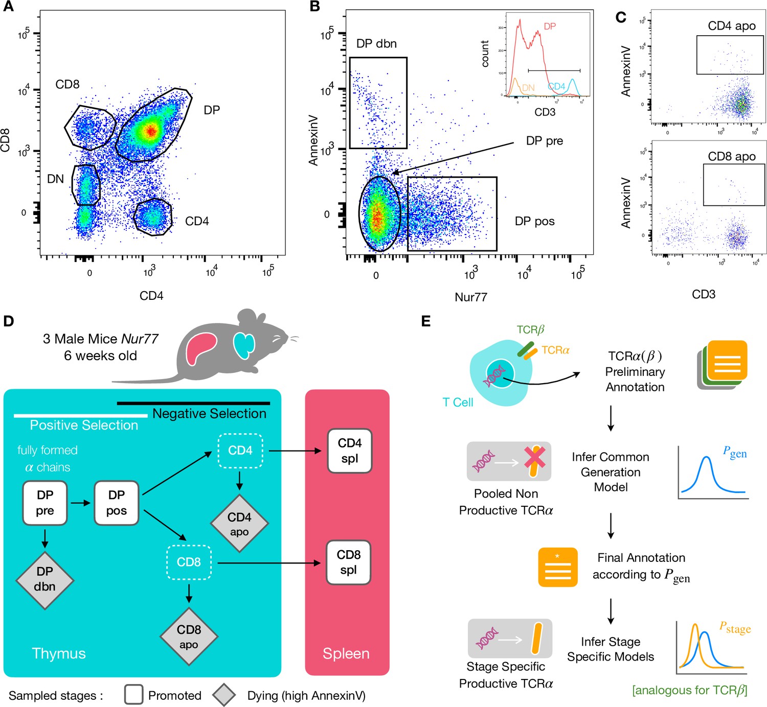
Experiment outline and repertoire sampling.
(A) Flow cytometry scatterplots of T cell population from the thymus according to the markers CD4 and CD8. (B) The DP population is separated from DN according to CD3 expression (insert). Cells are then FACS sorted according to the expression of Nur77 and AnnexinV. (C) CD4 cells in the spleen (above) and CD8 (below) are FACS sorted according to the expression of CD3 and AnnexinV. (D) Schematic evolution of the sampled cell types during thymic maturation. (E) Analysis workflow: annotated reads in sampled repertoires are input for model inference (see Materials and Methods). Out-of-frame TCR sequences are pooled from all mice and stages to learn a generation model. In-frame sequences are used to learn maturation stage specific selection models with the generation model as background.
Figure 1—figure supplement 1
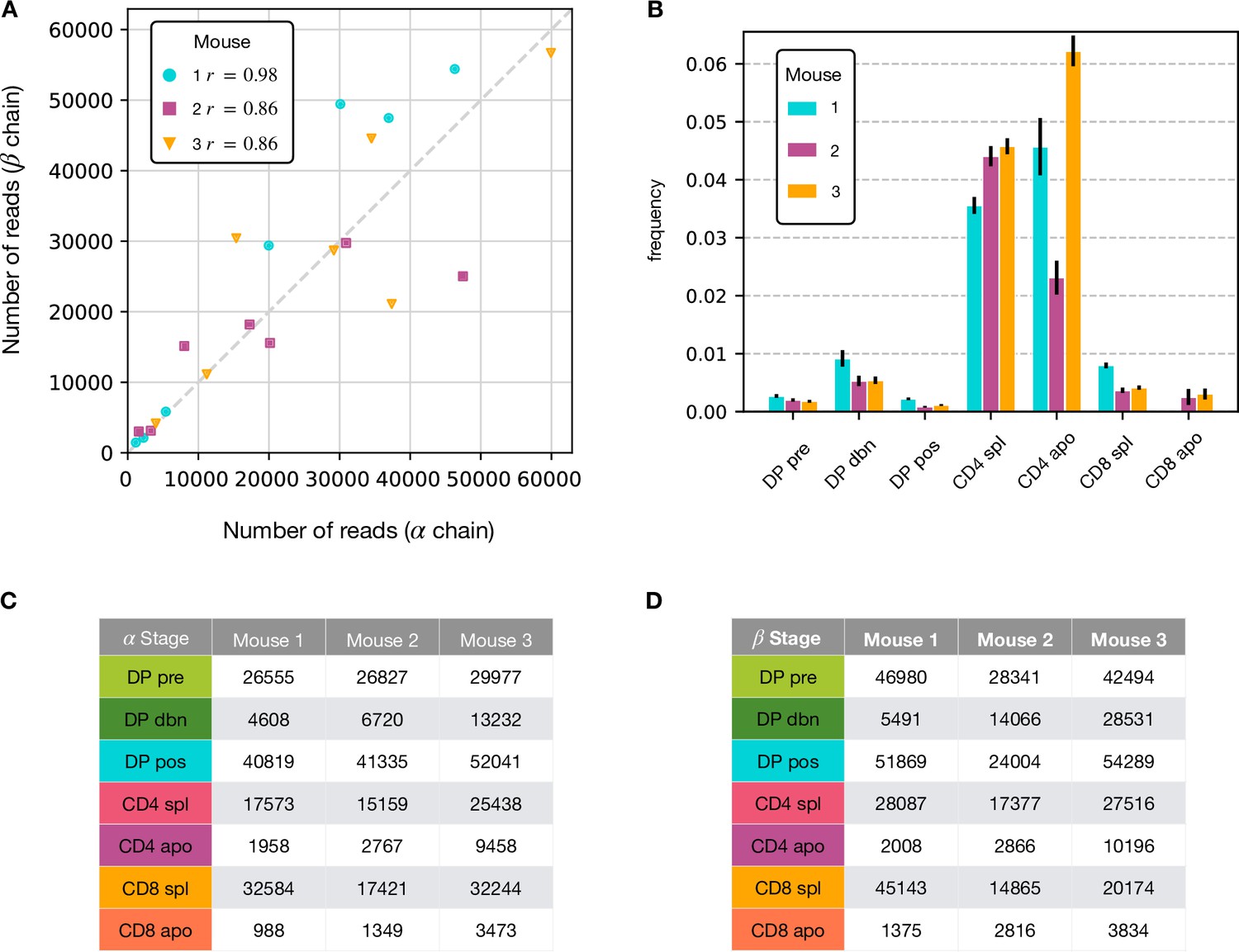
Summary of the RepSeq datasets.
(A) Number of reads for the alpha chain vs the number for the beta chain within the same dataset. In the box is shown the Pearson correlation coefficient. Distribution of iNKT clonotypes for the α chain. (B) The relative amount of (TRAV11, TRAJ18) clonotypes is significantly higher for all CD4 stages in all mice. (C) Numbers of unique productive (in-frame and with no stopping codons) single chain obtained for the maturation stages in each mouse after annotation for the α chain. (D) Numbers of unique productive for the β chain.
Figure 2 with 3 supplements
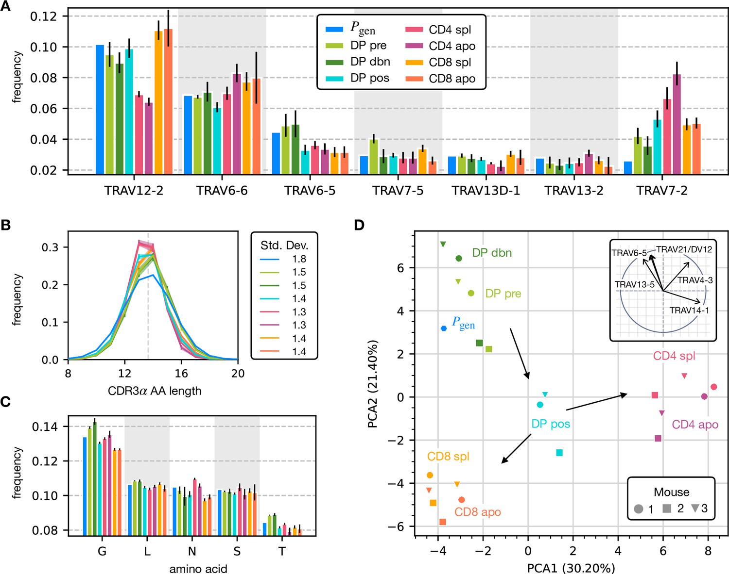
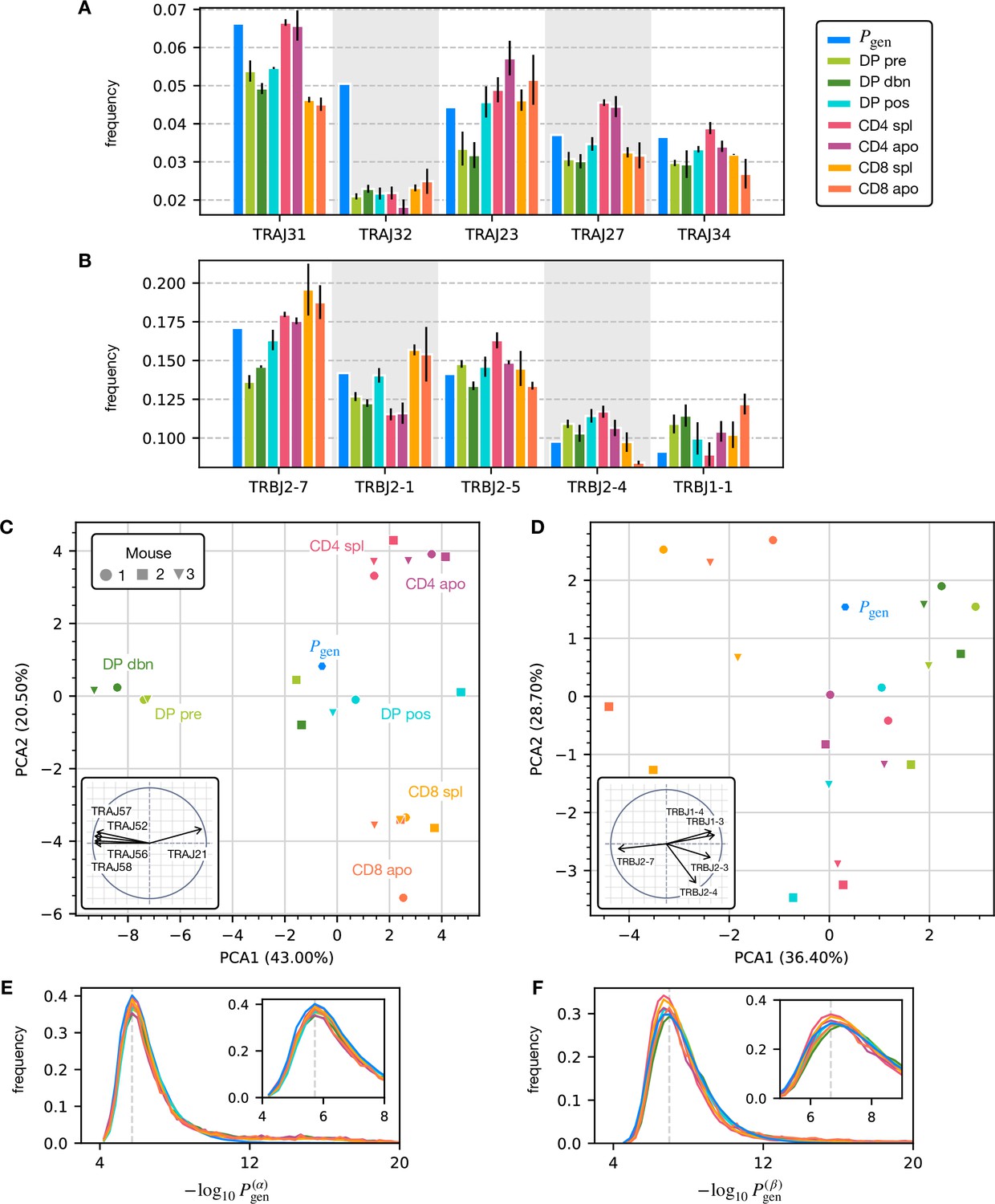
Properties of the α chain sequence (the analogous plot for the β chain is showed in Figure 2—figure supplement 1).
The color code is common to all subplots. (A) TRAV gene distribution at different maturation stages compared to the pre-selection model distribution (see Figure 2—figure supplement 2A for TRAJ). Only the most frequent according to the model are reported. Errorbars correspond to the empirical standard deviation across the three different mice. (B) CDR3 length distribution of TCRα sequences. The errors associated with mouse variability are minor and illustrated via the shaded curves. See Figure 2—figure supplement 3A for individual curves. The dashed line is the average CDR3 length from the model. Standard deviations of the average length distributions are shown at right. (C) Distribution of the most frequent amino acids at different maturation stages. The counts correspond to the number of observations within the CDR3 (i.e. excluding the first two and the last positions), summed for all the sequences in the subpopulation. Error bars represent the empirical standard deviation across mice. (D) Principal component analysis of the TRAV gene distribution at each maturation stage. Insert: projection on the principal axis of the five most abundant TRAV genes (see Materials and Methods). Analogous results for TRAJ are shown in Figure 2—figure supplement 2C. Source code available at https://github.com/statbiophys/thymic_development_2022/blob/main/fig2.ipynb.
Figure 2—figure supplement 1
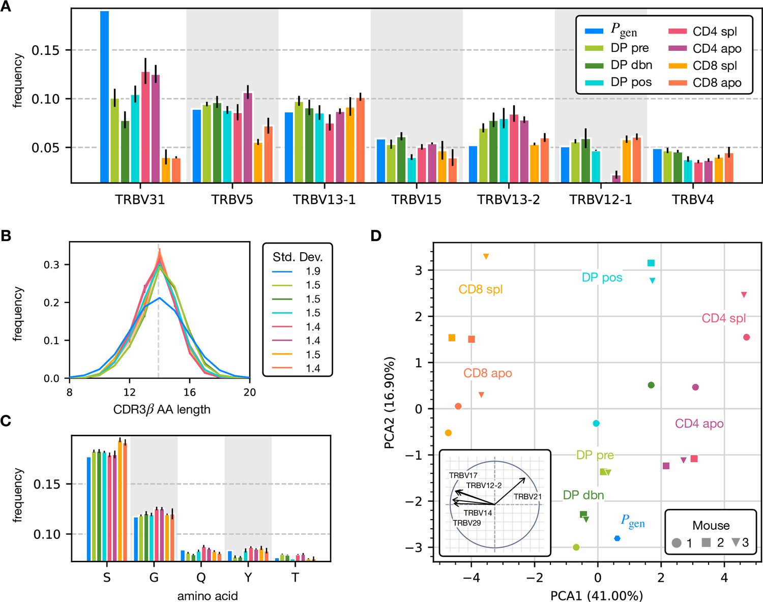
Analysis of the annotated productive β clonotypes for the different maturation stages.
(A) The distribution of TRBV genes at different maturation stages compared to the generation distribution. (B) Distribution of β chain CDR3 amino acid sequence lengths. The CDR3 is defined between the typical cysteine and phenylalanine position. The dashed line represents the average length according to the model. (C) The distribution of the most frequent amino acid within the CDR3 region for the TRBV sequences. (D) Principal component analysis according to the TRBV gene distribution at each maturation stage. Insert: projection on the principal axis of the five most representative TRBV genes. Analogous results for TRBJ are shown in Figure 2—figure supplement 2D.
Figure 2—figure supplement 2
Statistics of the J gene usage and the distributions.
(A) The distribution of J genes at different maturation stages compared to the generation distribution for the α chain. (B) The distribution of J genes for the β chain. (C) Principal component analysis of α chain J gene usage. Similarly as for the V genes (Figure 2C), DP, CD4 and CD8 maturation stages cluster by the cell types. (D) Principal component analysis of β chain J gene usage. (E) values distribution for the clonotypes at each maturation stage. Insert: blow up of the peak of the distribution (the dashed line) for the α chain. (F) values distribution the β chain.
Figure 2—figure supplement 3
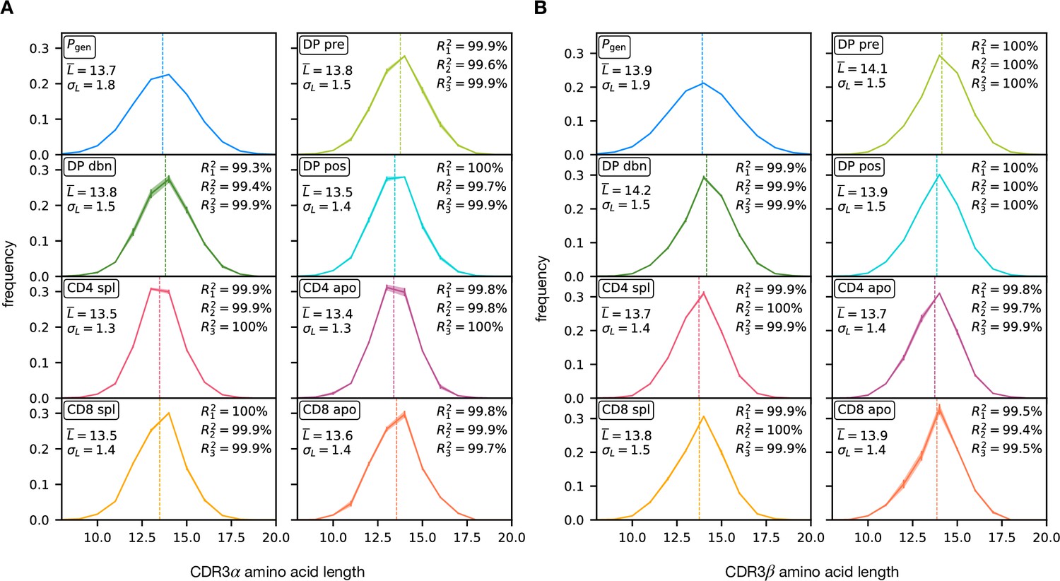
Separate amino acid CDR3 length distributions across all stages.
(A) Amino acid CDR3 length for TCRα sequences. The thick curve represent the average length across the three different mice, while the shaded part illustrates the mouse variability. On the left of each box, we report the empirical average and standard deviation of the distribution; on the right the coefficient of determination between each individual distribution and the average (see Materials and Methods). (B) Analogous for the TCRβ sequences.
Figure 3 with 2 supplements
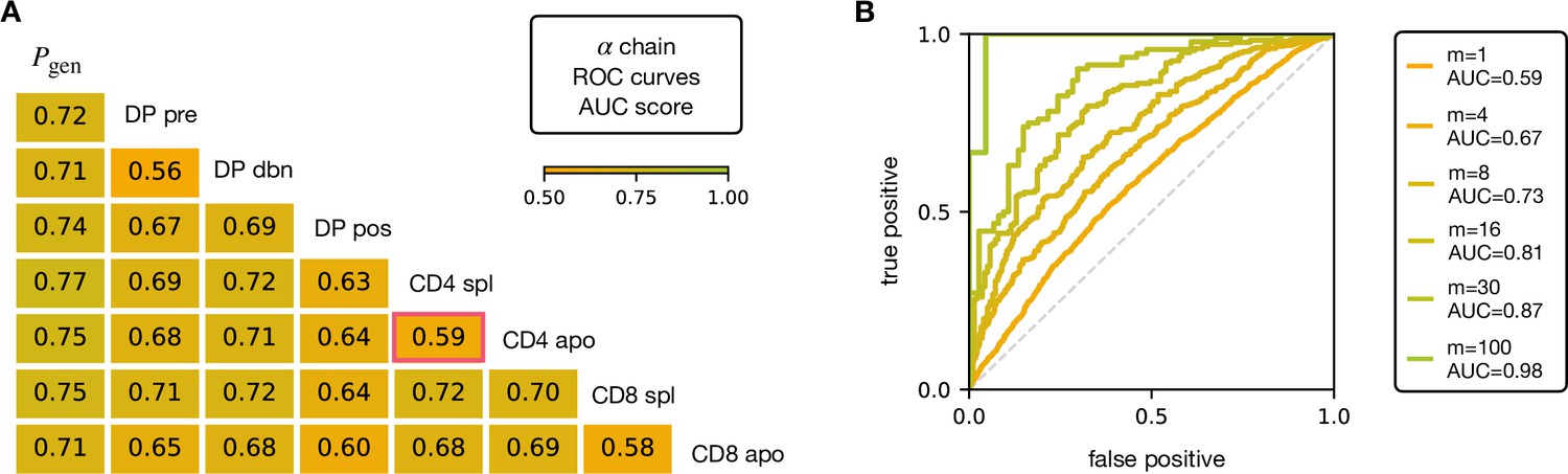
AUC scores for the pooled TCRα datasets.
(A) Area under the curves (AUC) values computed from Receiver Operating Characteristic (ROC) curves of linear classifiers of TCRα between two subsets. The training/testing set is a random subsample containing 70%/30% of the full dataset at a given maturation stage. (B) ROC curves for classifying a group of sequences from the same maturation stage, between CD4 spl and CD4 apo (red frame in A), illustrating the improvement with increasing number of TCRs. See Figure 3—figure supplement 1 and (B) for the analogous analysis on TCRβ. Source code available at https://github.com/statbiophys/thymic_development_2022/blob/main/fig3.ipynb.
Figure 3—figure supplement 1
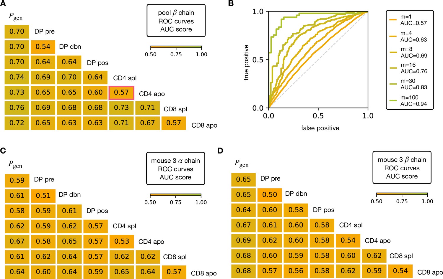
AUC scores for the pooled TCRβ datasets and for an individual mouse.
(A) AUC values computed from the ROC curves of the linear classifiers for TCRβ sequences between pairs of maturation stages. The training/testing set is a random subsample containing 70%/30% of the full dataset at a given maturation stage. (B) Illustration of the improvements of group discriminability between the stafes CD4 spl and CD4 apo. (C) AUC values computed from the ROC curves of the linear classifiers for TCR sequences for the unpooled largest dataset for an individual (mouse 3). We observe that the score is never higher than for the pooled case and in fact it’s tipically worse for the α chain. (D) Analogous for the β chain.
Figure 3—figure supplement 2
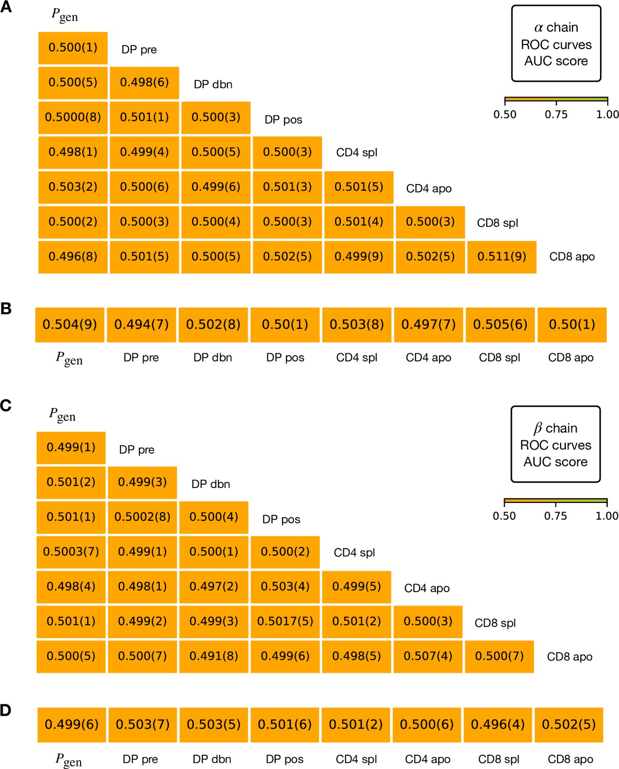
Validation of the stages discrimination.
Here we organize the different train/test datasets as in the main text (Figure 3) and we learn logistic regression classifiers as in Materials and Methods, of which we report the AUC score. Analogous results are obtained by usage of a random decision forest. (A) We randomly shuffle the labels for each pair of α stages, observing that it is impossible to obtain two distinguishable repertoires through random mixing. The error for the last digit is expressed in brackets and is obtained from 20 realizations of the shuffling. (B) We randomly assign two labels to the TCRα sequences of a single repertoire and split the repertoire in a test and a train group. Again, we show that it’s not possible to obtain the scores of the main text by randomly pick chains from a defined stage. In all these controls we sub-sampled to the size of the smallest dataset available in order to check for issue size. As in the main text (see Materials and Methods), we test linear and decision forest classifiers, imposing the size of the larger class to not exceed of more then 25% the size of the smaller, with the test set corresponding to 30% of data. (C) Classifiers learnt on pair of β stages with randomly shuffled labels. (D) Classifiers learnt on single βstages with randomly assigned labels.
Figure 4 with 8 supplements
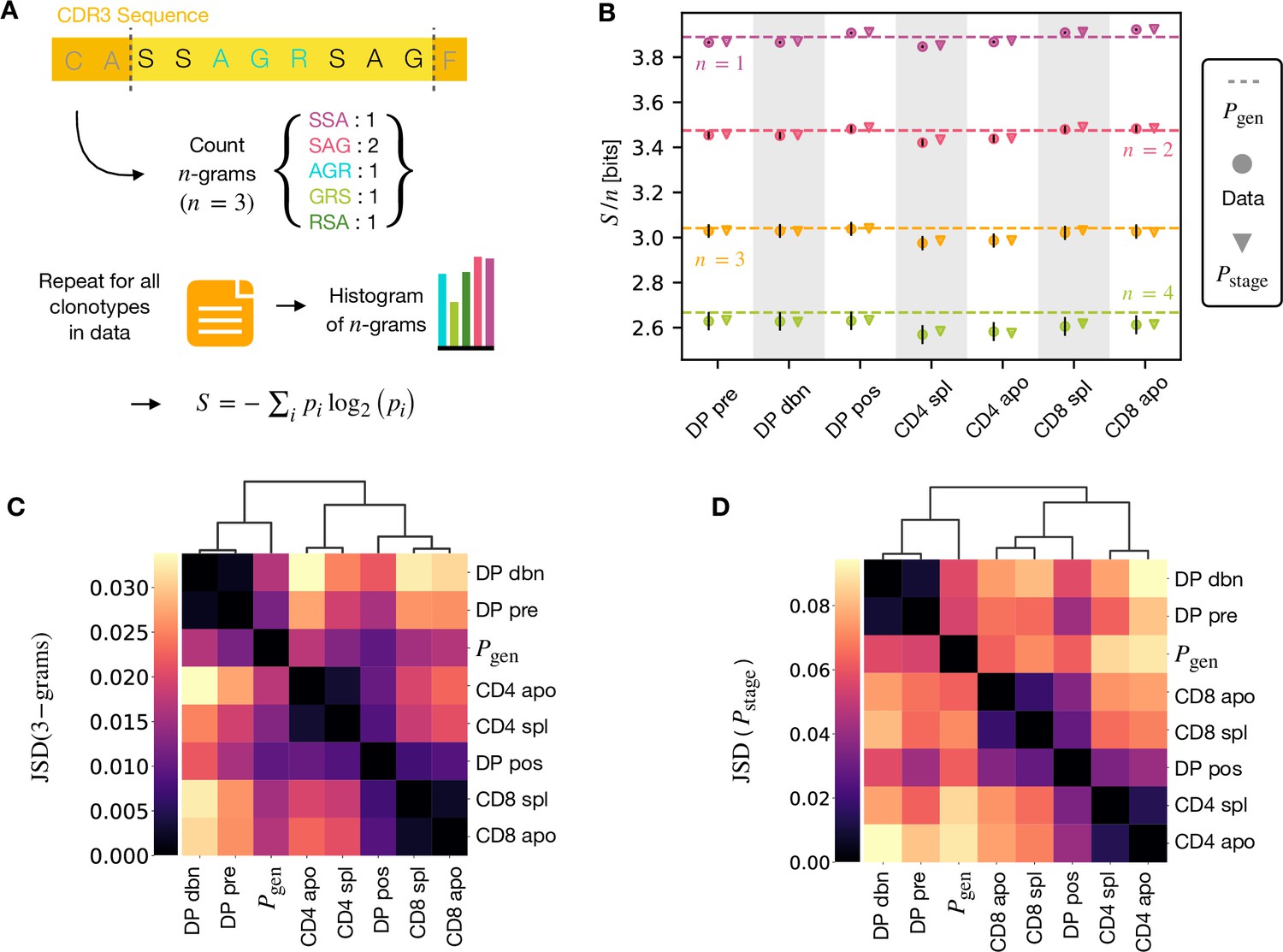
-gram frequency discriminates between repertoires.
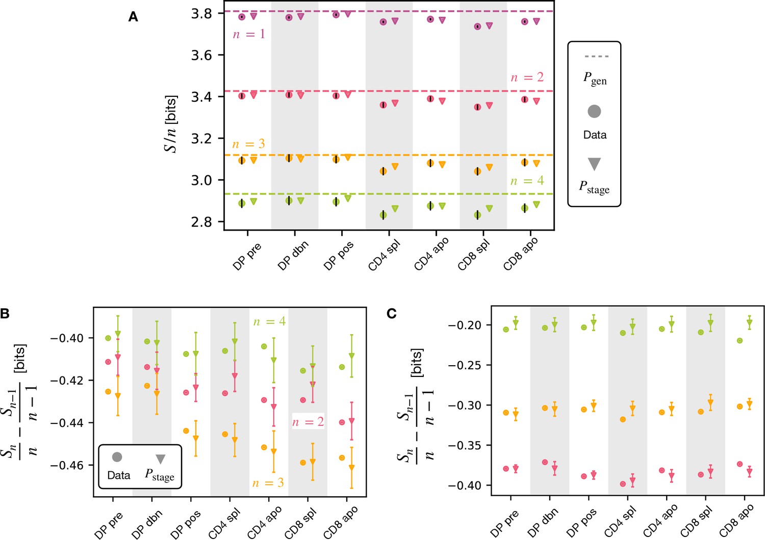
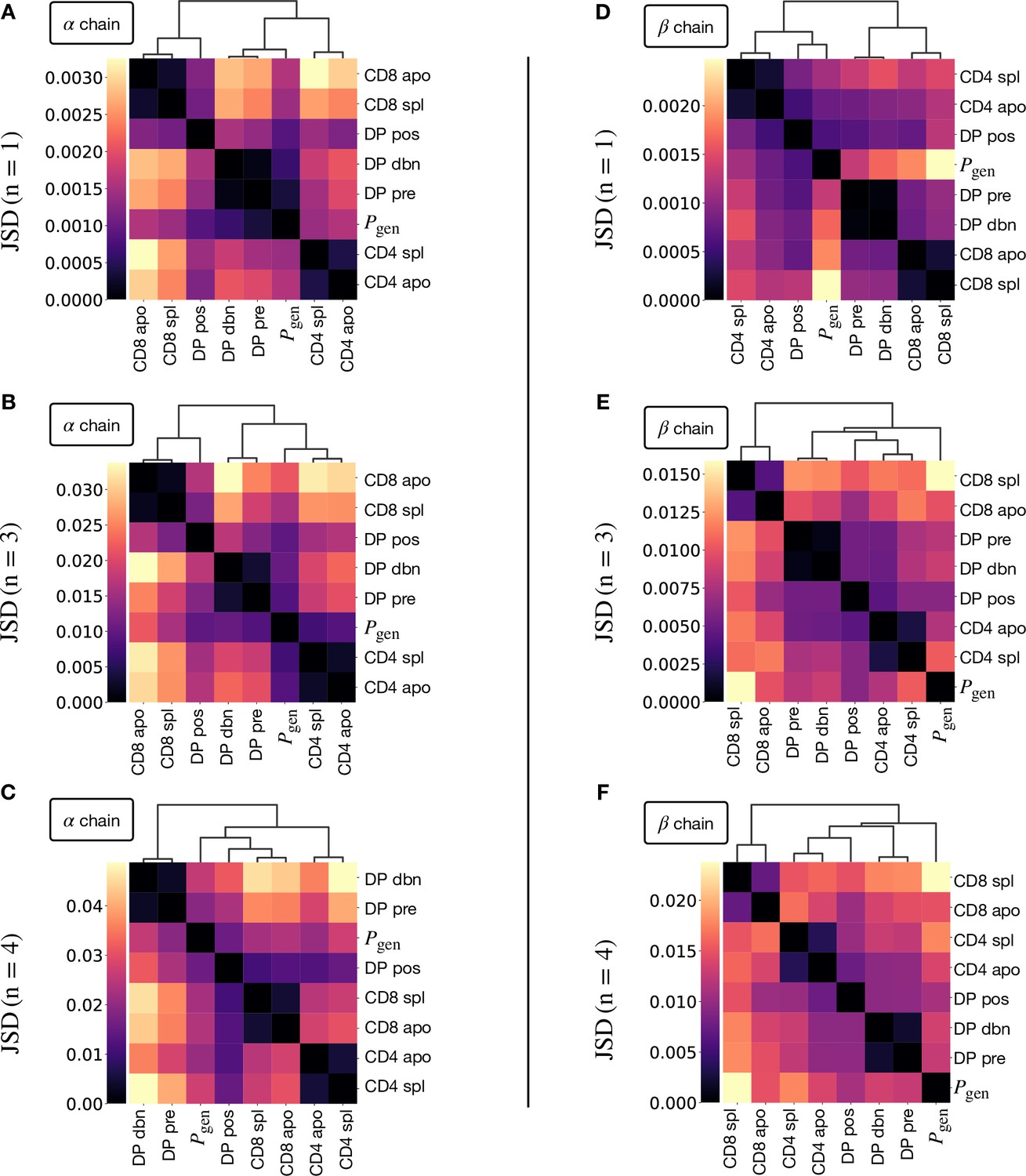
(A) -gram definition. We count how many times -gram amino acid subsequences are seen in the CDR3 across a repertoire. (B) Shannon entropy of the -gram distributions normalized by for the maturation stages. The entropy is estimated with the Nemenman et al., 2002 estimator and it is expressed in bits. The error on the estimated Shannon entropy from data is estimated from the sequencing error (see Materials and Methods). (C) Clustering according to Jensen-Shannon divergence between the 3-gram distributions computed from the selection model on synthetic repertoires. Dendrogram are computed with the Ward method (see Materials and Methods). (D) Clustering based on Jensen-Shannon divergence for the full selection model using . Source code available at https://github.com/statbiophys/thymic_development_2022/blob/main/fig4.ipynb.
Figure 4—figure supplement 1
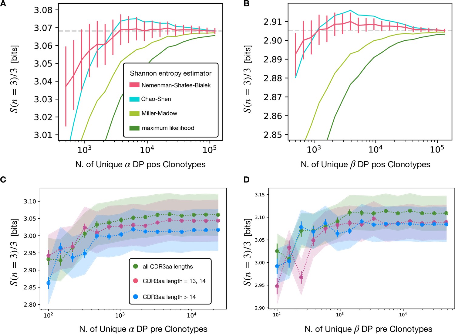
Comparison of different entropy estimators and of the dependence on the CDR3aa length choice.
(A) Averages over different subsamples of the same size for productive DP pos pooled clonotypes. The estimators compared are: Nemenmann-Shafee-Bialek (see Materials and Methods) (Nemenman et al., 2002, Chao and Shen, 2003, Miller, 1955) and maximum likelihood (naive estimator). (B) Analogous for the β chain. (C) Analysis of the length dependence of 3gram entropy associated to different choices of th CDR3 amino acid lengths for the clonotypes considered in the α DP pre stage. The errorbars are estimated with the NSB method, while the shaded curve represent the sequencing error. We notice how the difference between the different choices is greatly covered by the sequencing error. We prefer then to use all CDR3 lengths for the higher statistics. (D) Analogous for the β chain.
Figure 4—figure supplement 2
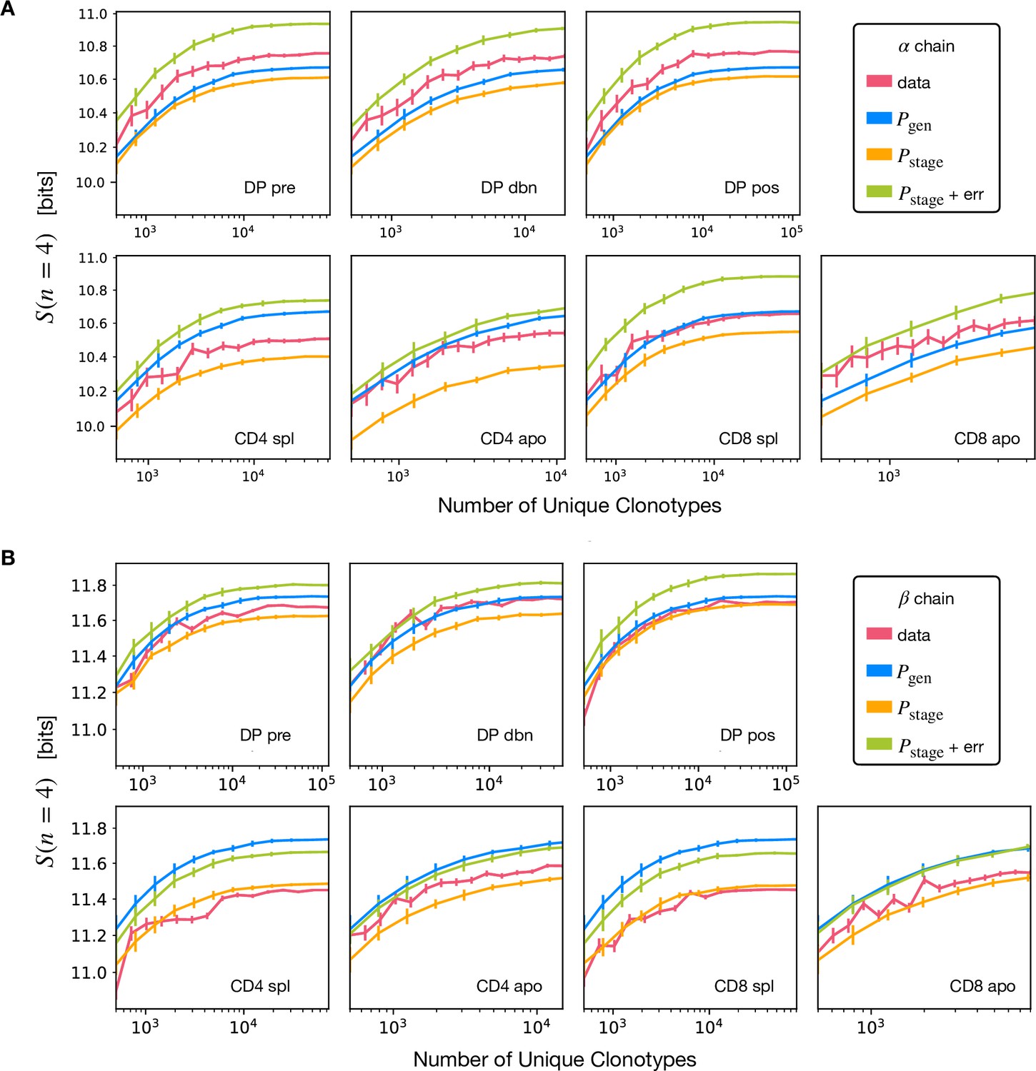
Convergence of the -gram entropy estimations.
(A) We subsample the unique clonotypes for the TCRα sequences and we check that the 4-gram entropy estimations converge with increasing number of unique clonotypes. The synthetic sequences are produced with the generation model (same for all plots), the different selection models and a selection model with synthetic nucleotide sequencing error. The estimation is performed using the Nemenman-Shafee-Bialek (NSB) estimator. The error bars for data are obtained with the NSB method, while for synthetic sequences are estimated as the empirical standard deviation over different realizations of the simulation. Due to the increased statistics, the convergence is faster for (the number of possible -grams grows as 20n, thus we decided to show this analysis only for the case ). (B) Analogous analysis for TCRβ sequences.
Figure 4—figure supplement 3
Shannon entropy on β-grams and entropy dependency on .
(A) NSB estimation of the Shannon entropy normalized by , associated to -gram distributions within the CDR3 TCRβ chain of unique clonotypes from the different maturation stages. The error bars for the data are estimated from the sequencing error. (B) Decrease in entropy per symbol between and grams for the α chain. The decreases are comparable. The errorbars associated to simulation are obtained as the same of the two standard deviations as returned by the NSB estimator. (C) For the β chain the decreases get smaller with .
Figure 4—figure supplement 4
Jensen-Shannon divergence between -gram distributions.
(A) Jensen-Shannon divergence (Equation 8) for different -gram distributions (here ) estimated on synthetic TCRα repertoires for different maturation stages. The dendrogram is computed with the Ward method (see Materials and Methods). (B) Divergence for TCRα in the case . We report here the same figure shown in the main text for the sake of comparison (Figure 4C). (C) Divergence for TCRα in the case . (D) Divergence for TCRβ in the case . (F) Divergence for TCRβ in the case . (G) Divergence for TCRβ in the case .
Figure 4—figure supplement 5
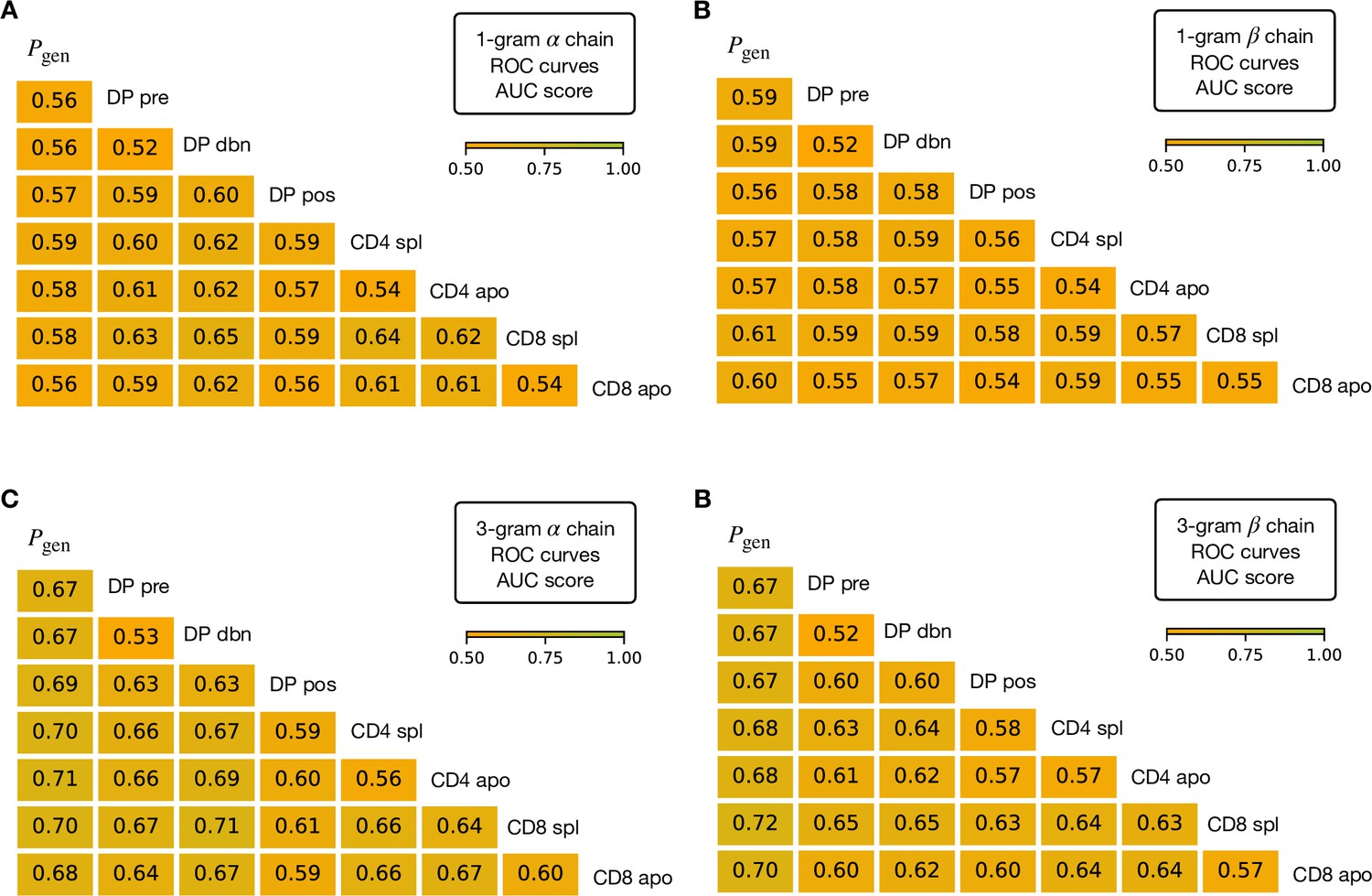
AUC values computed from the ROC curves of the linear classifiers learnt over n-grams features.
(A) 1gram classifiers for the α chain. In the case of 1-grams, the features are assigned according to the counts of appearance of a certain amino acid within the CDR3 region (20 features). (B) 1-gram classifiers for the β chain. (C) 3-gram classifiers for the α chain. In the case of 3-grams we choose a one-hot-encoding of the 8000 features. We observe the increased discrimination power of the 3-grams with respect to 1-gram as expected, the latter being generally worse than the models learnt on top of Sonia features. (D) 3-gram classifiers for the β chain.
Figure 4—figure supplement 6
Measure of the Shannon entropy using the full stage models.
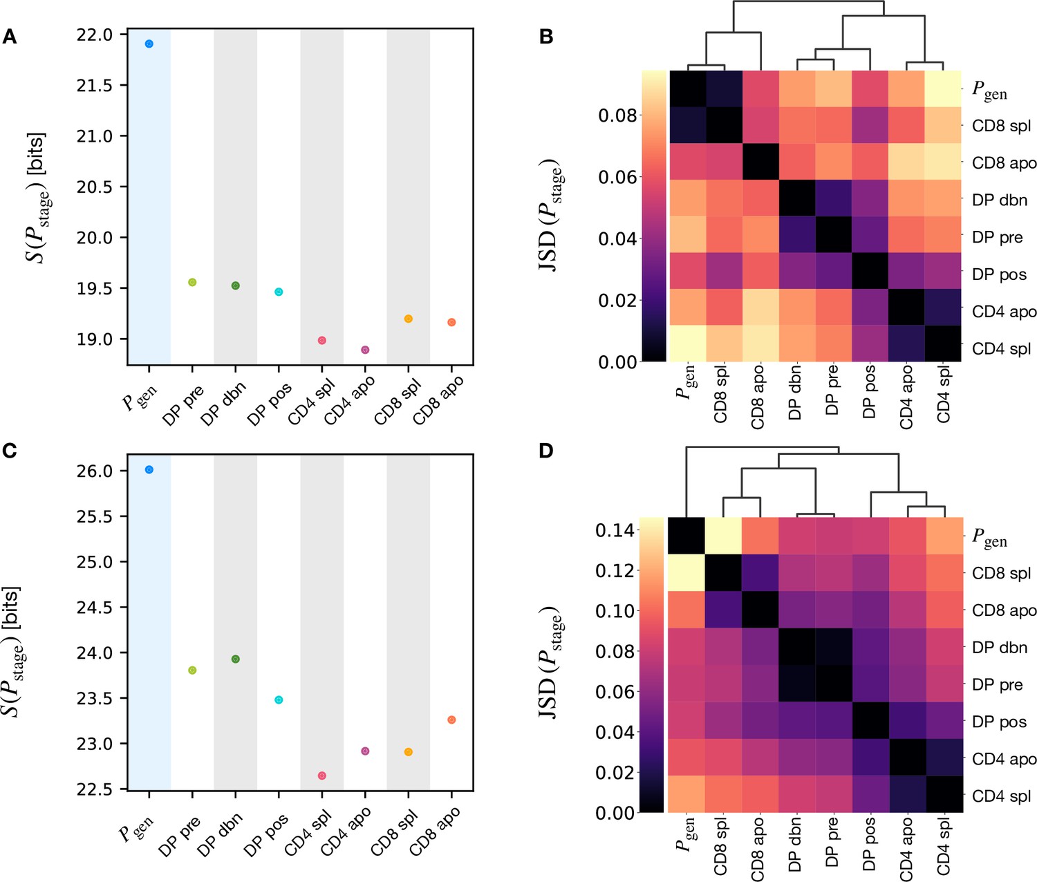
(A) Shannon entropy estimation associated to the full model for the α chain (Equation. 7) for the different selection models and the generation model. (B) We report here the same figure shown in the main text for the sake of comparison (Figure 4D). (C) Shannon entropy estimation associated to the full model for the β chain for the different selection models and the generation model. (D) Jensen-Shannon divergence for the β chain models.
Figure 4—figure supplement 7
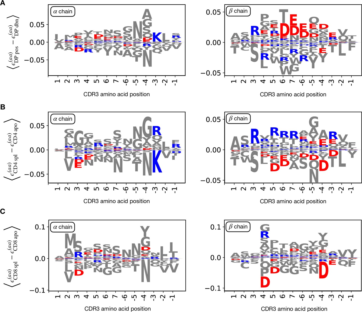
Logo plots for the relative enrichment of positional amino acid usage.
(A) Logo plots for the CDR3 amino acid usage inferred by the model, from the left (positive position indexes) and from the right (negative), omitting the first and the last one. Here the quantity represents the average difference between weights associated to amino acid at the given position by models (see Materials and Methods). Analogously with the energy difference, a negative difference implies the feature is favoured in stage 1, vice versa for stage 2. We follow the color scheme from Tubiana et al., 2019 to highlight the charge properties (red for positive charge, blue for negative charge). On the left is shown the weights difference between stages DP pos and DP dbn for the α chain. For the β chain (right) we see a reduction of positively charged amino acid in DP pos. (B) Stages CD4 spl and CD4 apo. Conversely, here the CD4 spl stage show enhancement in positively charged for the β chain (right). (C) Stages CD8 spl and CD8 apo. We observe just a slight enhancement of positively charged amino acid in CD8 spl.
Figure 4—figure supplement 8
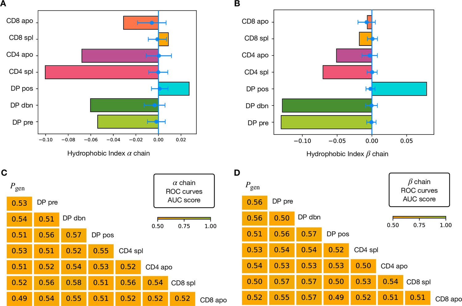
Hydrophobic score at different stages and AUC scores of classifiers on hydrophobic features.
(A) We measure the increase of hydrophobicity from the generation benchmark using a stage-wide score defined from the inferred models (see Materials and Methods, Equation 4). As a control, we compute the same quantity over a set of models learnt on -generated repertoires of the same sizes (in blue). The error bars correspond to the standard deviation over 25 repetitions. The score is showed at the various stages for the α chain. We observe a clear increase from DP pre to DP pos and a subsequent decrease for the single positive sets, in agreement with the role of positive and negative selection. (B) Analogous analysis for the β chain. In this case we also observe AnnexinV+ sets with a higher score than the spleen sets. (C) AUC scores computed from the ROC curves of the logisitc regression classifiers learnt over an empirical hydrophobic index of the α repertoires (see Materials and Methods, Equation 5). (D) AUC scores for the classifiers on on hydrophobic features for the β chain.
Figure 5 with 1 supplement
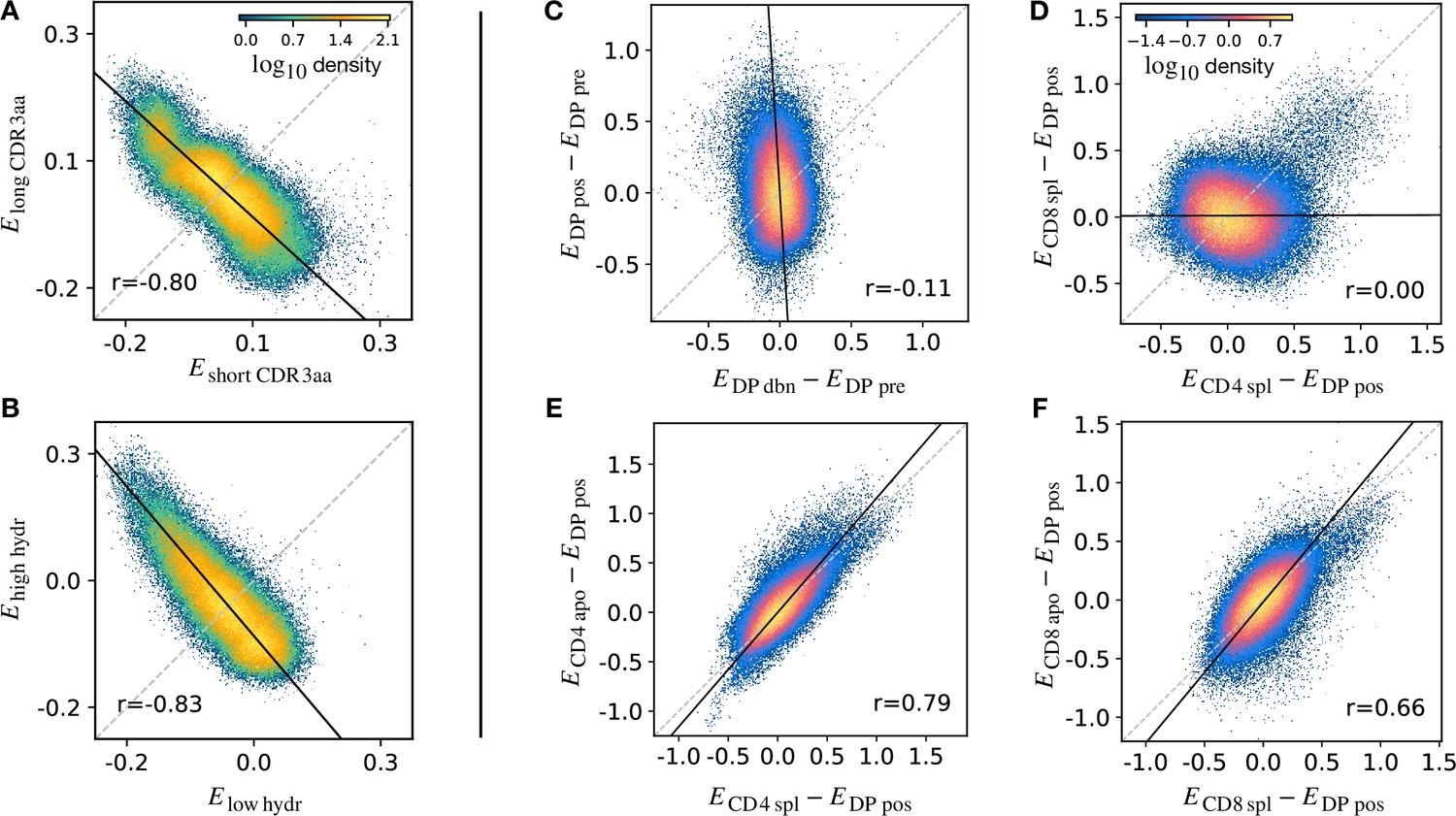
Density scatter-plots of TCRα sequences comparing the selection energies learnt at two different stages.
(A) Synthetic example of soft discrimination between ‘short’ and ‘long’ CDR3, where sequences are randomly assigned into either of the two populations with a bias that depends on their CDR3 length. The density scatter plot shows a clear anti-correlation between the selection energies learnt from these two populations. Yet, sequence classification is imprecise, as quantified by the low AUC = 0.57. The parameters chosen for the filter in this example are and . (B) Synthetic example of soft discrimination between ‘low’ and ‘high hydrophobic’ CDR3 showing clear anti-correlation between these two populations. Sequence classification is again poor AUC = 0.60. The parameters chosen for the filter on the ‘hydrophobic index’ in this example are (the median value over a set of -distributed sequences) and . (C) The differential enrichment parameter of each TCR calculated according to model is plotted against the energy calculated against the model. To correct for bias imposed by the TCRα generation process, the DP pre energy, which encodes background selection common to both stages, is subtracted. The black line is the direction of the major eigenvector of the dots moments matrix. The value reported in each plot is the Pearson’s correlation coefficient (see Materials and Methods). (D) Differential enrichment parameter according to CD4 spl and CD8 spl models, relative to DP pos. (E) Differential enrichment parameter according to CD4 spl and CD4 apo models, relative to DP pos. (F) Differential enrichment parameter according to CD8 spl and CD8 apo models, relative to DP pos. Source code available at https://github.com/statbiophys/thymic_development_2022/blob/main/fig5.ipynb.
Figure 5—figure supplement 1
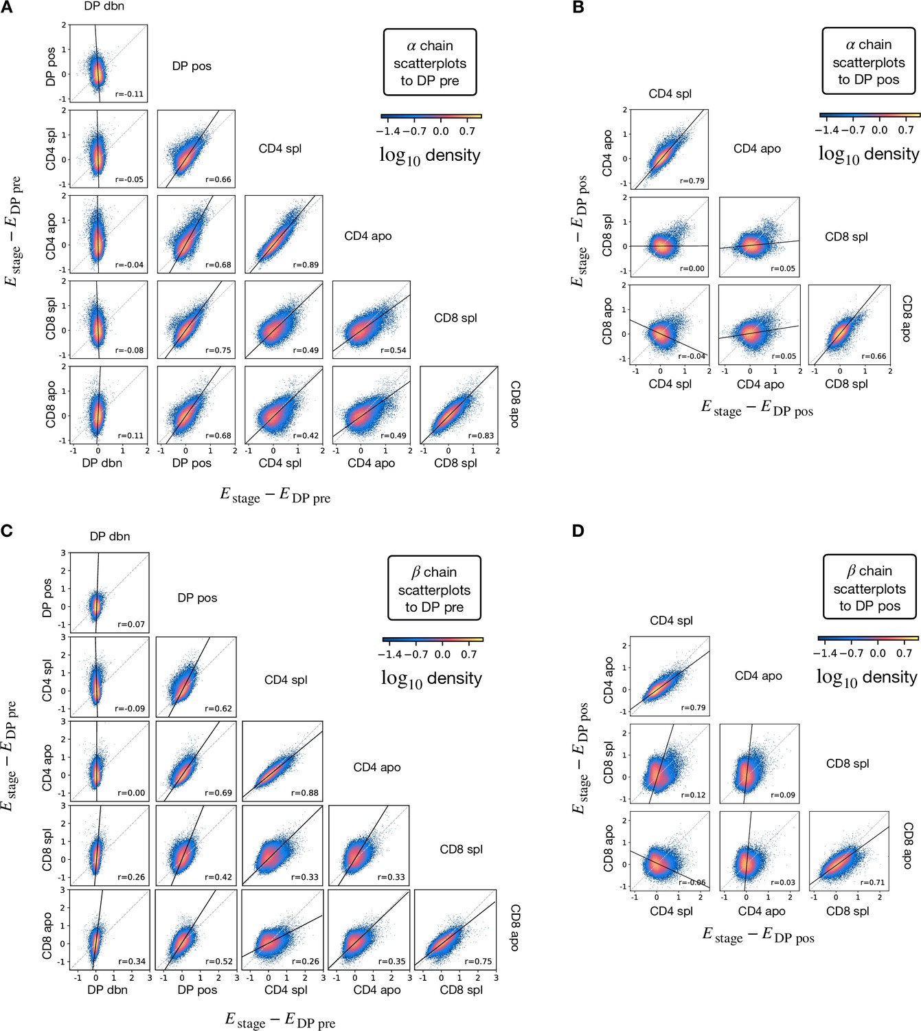
Differential increments scatterplots for all pairs of stages.
The differential enrichement parameters assigned by the stage specific selection models relative to the the preceding stage (i.e. energy differences from DP pre or DP pos). Each dot represents one of the 3.106 synthetic sequences generated according to the generation model , here shown according to a dot density plot. Each figure uses the same set of synthetic sequences. (A) Density scatterplots of the energy differences between the energies of the TCRα models and the enregy of DP pre. (B) Density scatterplots for TCRα where DP pos energy is subtracted instead. (C) Density scatterplots for TCRβ where DP pre energy is subtracted. (D) Density scatterplots for TCRβ where DP pos energy is subtracted.
Tables
Table 1
Cell sorting based on fluorochrome-labeled mouse antibodies.
| Sample\Marker | CD4 | CD8 | CD3 | AnnexinV | Nur77 |
|---|---|---|---|---|---|
| DP pre | + | + | + | - | - |
| DP pos | + | + | + | - | + |
| DP dbn | + | + | + | + | - |
| CD4 apo | + | - | + | + | |
| CD8 apo | - | + | + | + |
Additional files
-
MDAR checklist
- https://cdn.elifesciences.org/articles/81622/elife-81622-mdarchecklist1-v2.pdf
-
Supplementary file 1
Primers list.
- https://cdn.elifesciences.org/articles/81622/elife-81622-supp1-v2.xlsx
-
Supplementary file 2
Cell counts.
- https://cdn.elifesciences.org/articles/81622/elife-81622-supp2-v2.xlsx
Download links
A two-part list of links to download the article, or parts of the article, in various formats.
Downloads (link to download the article as PDF)
Open citations (links to open the citations from this article in various online reference manager services)
Cite this article (links to download the citations from this article in formats compatible with various reference manager tools)
Quantifying changes in the T cell receptor repertoire during thymic development
eLife 12:e81622.
https://doi.org/10.7554/eLife.81622


