Spatial frequency representation in V2 and V4 of macaque monkey
- Department of Neurosurgery of the Second Affiliated Hospital, Interdisciplinary Institute of Neuroscience and Technology, School of Medicine, Zhejiang University, China
- Key Laboratory of Biomedical Engineering of Ministry of Education, College of Biomedical Engineering and Instrument Science, Zhejiang University, China
- MOE Frontier Science Center for Brain Science and Brain-Machine Integration, School of Brain Science and Brain Medicine, Zhejiang University, China
Figures
Figure 1

Illustration of proposed hypercolumn (including spatial frequency [SF], color, and orientation domains) in the visual cortex.
(A) As eccentricity decreases from parafoveal to foveal region, the preferred SF gradually increases (represented as the brightness of the short bar). However, a local region (marked by a rectangle) covers a full range of SF representations in its corresponding topographic locations. This local region can be considered a ‘hypercolumn.’ (B) Details of structure in a single hypercolumn. In this local region, color domains (orange area) and orientation domains (blue area) exhibit different relationships with SF domains (light gray region: low SF preference domain; dark gray region: high SF preference domain). Orientation maps orthogonally to SF maps (green dashed lines: iso-orientation contours; purple dashed lines: iso-SF contours); an extensive range of SFs are available to each orientation. In comparison, color domains tend to have more spatial overlap with low SF preference domains and avoid overlap with high SF preference domains. In color domains, another orthogonal relationship exists between hue (dotted lines with different colors: iso-hue contours) and brightness (blue dashed lines: iso-brightness contours).
Figure 2
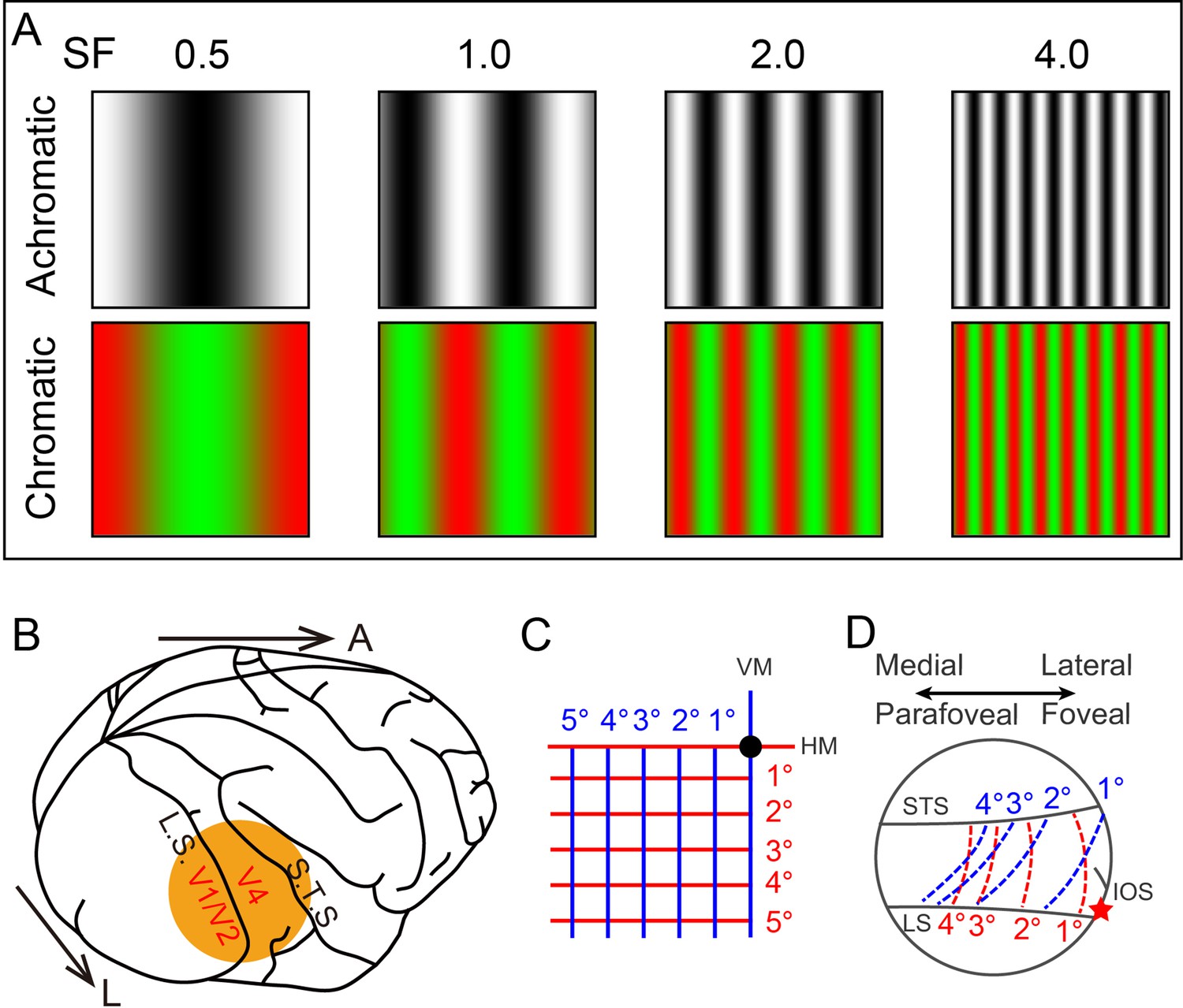
Experimental parameters.
(A) Visual stimuli. Top and bottom rows show the black/white and green/red full screen sinusoidal gratings for four different spatial frequencies (SFs) (indicated by the numbers on top, in cycles/deg). Here for demonstration, the stimulus size is set to 2°. (B) Diagram of imaging site in the right hemisphere. L: lateral; A: anterior. (C) Lower-left visual field. Black dot: fovea. Horizontal (red) and vertical (blue) lines mapped in (D). (D) Schematic mapping of lines in (C) in V4 (corresponding to the orange disc in B). The lateral part of the imaged region corresponds to the foveal region, while the medial part corresponds to the parafoveal region. LS: lunate sulcus; STS: superior temporal sulcus; IOS: inferior occipital sulcus. Red star: estimated foveal location.
Figure 3 with 1 supplement
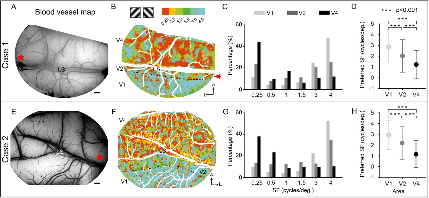
Two examples of overall spatial frequency (SF) preference in visual cortex.
(A, E) Blood vessel map of the imaged region for cases 1 and 2, respectively. V2 and V4 are separated by the lunate sulcus (LS). Red star: estimated foveal location. Scale bar here and in all subsequent figures are 1 mm. (B, F) SF preference maps for cases 1 and 2, respectively. Each SF stimulus contains two orientations, 45º and 135º. For each pixel, the preferred SF is defined as the SF corresponding to its strongest response. Different colors represent different SF preferences (see color bar at top). The border between V1 and V2 (defined by ocular dominance image) is indicated by a black dashed line. A, anterior; L, lateral. (C, G) The coverage ratio of SF preference in each visual cortical area (light gray: V1; medium gray: V2; black: V4). (D, H) Mean ± SD for the preferred SF of all pixels across V1, V2, and V4. ***Kolmogorov–Smirnov test, p<0.001.
Figure 3—figure supplement 1
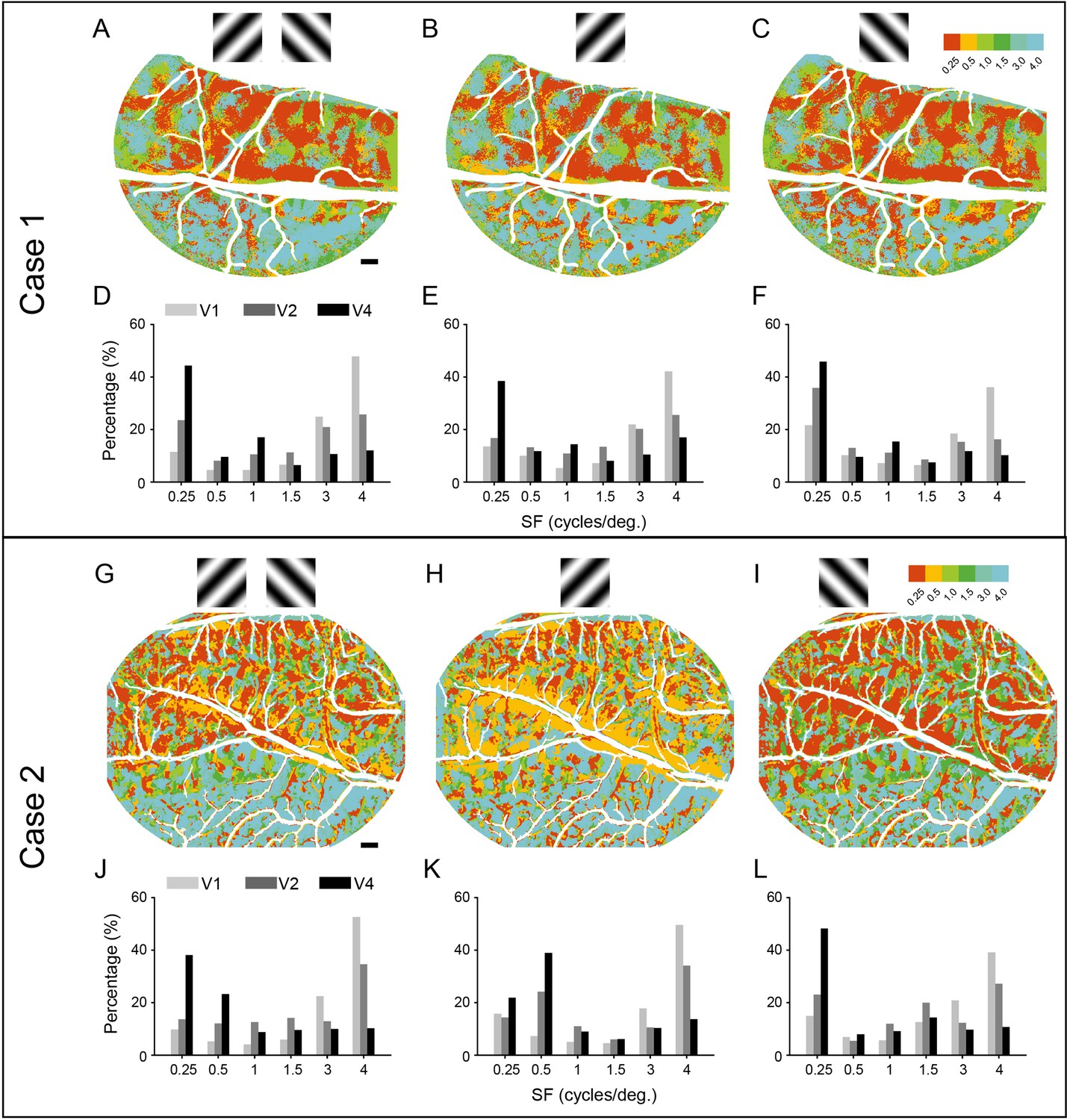
Two examples of spatial frequency (SF) preference maps obtained with different orientations (A–F: case 1; G–L: case 2).
(A–C, G–I) SF preference maps obtained by different orientations (A, H: 45° and 135°; B, H: 45°; C, I: 135°). The color bar represents the preferred SF from 0.25 (red) to 4.0 (cyan) cycles/deg. Scale bars here and for all subsequent figures are 1 mm. (D–F, J–L) Preferred SF distribution acquired by different orientations and areas. The orientation factor does not cause significant differences (two-way ANOVA, p>0.05) in the results of the SF preference (SF = 0.25), (4), while the area factor causes significant differences (two-way ANOVA, P<0.05). Two-way ANOVA test. case 1: area difference (V1, V2, V4), p=0.0029 (SF = 0.25 cycles/deg); p=0.0008 (SF = 4 cycles/deg); orientation difference (45 + 135°, 45°, 135°), p=0.057 (SF = 0.25 cycles/deg); p=0.063 (SF = 4 cycles/deg). Case 2: area difference (V1, V2, V4), p=0.040 (SF = 0.25 cycles/deg); p=0.00061 (SF = 4 cycles/deg); orientation difference (45 + 135°, 45°, 135°), p=0.27 (SF = 0.25 cycles/deg); p=0.12 (SF = 4 cycles/deg).
Figure 4 with 3 supplements
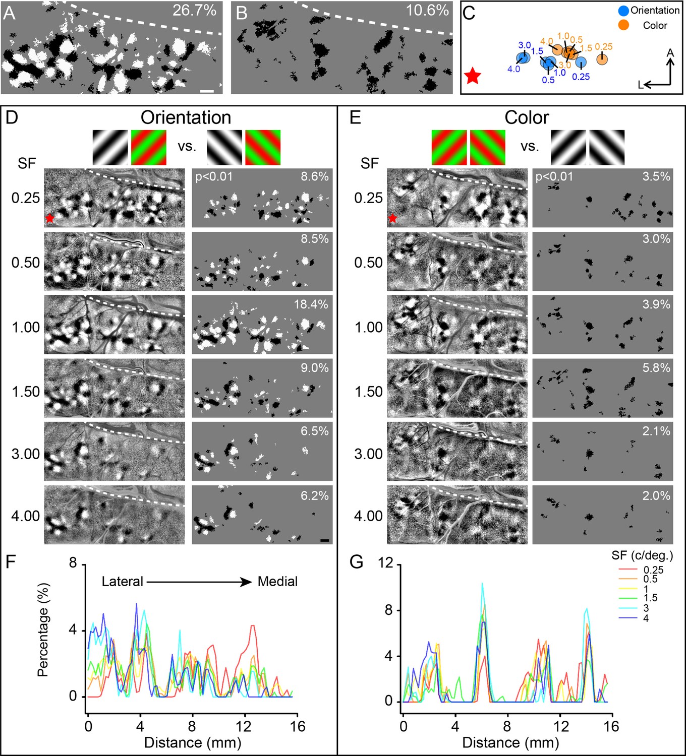
Comparison of the functional maps obtained at different spatial frequencies (SFs).
(A, B) Combined results generated by superimposing pixels in (D) and (E), respectively. Scale bar, 1 mm. (C) Selective activation centers of the activated orientation domains (blue dots) and color domains (orange dots) under different SF conditions. The dots are the geometric centroid of all corresponding activated regions in V4 (two-tailed t-test, p<0.01). The values indicate the SF used. (D) V4 orientation maps and corresponding activated regions for different SFs. The gratings above the maps indicate the subtraction pair for the maps. Left panel: differential maps in response to 45° (black patches) versus 135° (white patches); right panel: stimulus-activated orientation-selective regions, only pixels that can distinguish 45° (black pixels) from 135° (white pixels) are included (two-tailed t-test, p<0.01), numbers in the top-right corner indicate the coverage ratio of activated regions in the imaged V4. Red star: estimated foveal location. (E) Color maps and corresponding activated regions for different SFs, acquired from the same case in panel (A). Gratings above the maps indicate the subtraction pair for the maps. Left panel: differential maps in response to R/G gratings (corresponding to the black patches) versus W/B gratings (corresponding to the white patches). Right panel: activated color preference regions for the stimuli, only pixels showing significantly stronger responses to R/G gratings (black pixels) are included (two-tailed t-test, p<0.01). (F, G) Activated area histograms along the M-L axis generated from (D) and (E), respectively.
Figure 4—figure supplement 1
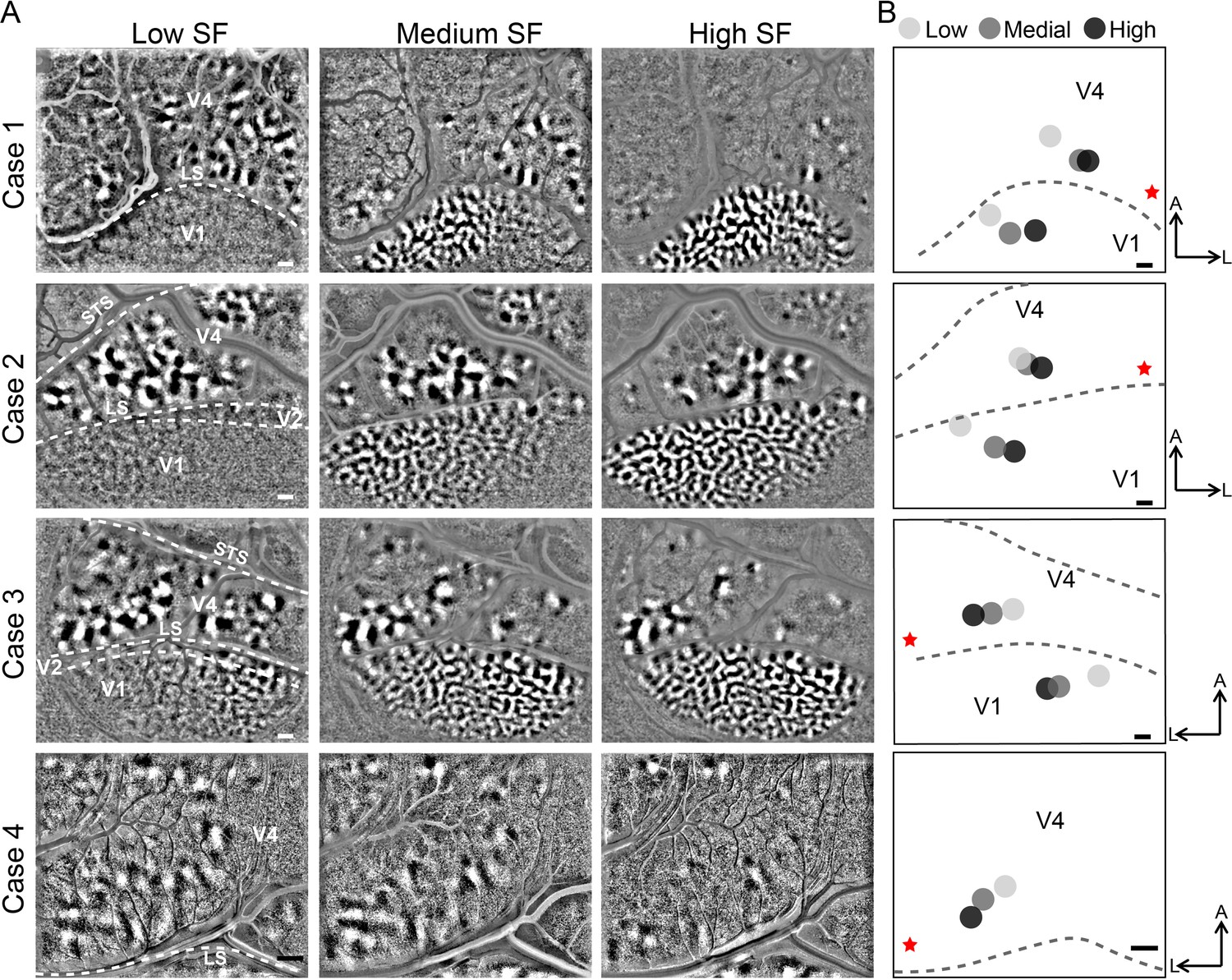
Orientation maps obtained by using drifting gratings with different spatial frequencies (SFs).
(A) Imaging results of cortical responses to gratings with different SFs (indicated on top in each column). Maps generated from response difference of 45° gratings minus 135° gratings (each row represents results from different cases). LS, lunate sulcus; STS, superior temporal sulcus. (B) Spatial distribution of the geometric center of activated orientation domains with different SFs. Under different SF conditions, the geometric centers of the activated orientation domains were calculated (two-tailed t-test, p<0.01). Light gray: low SF, 0.25–0.5 cycles/deg; gray: medium SF, 1–2 cycles/deg; dark gray: high SF, 3–4 cycles/deg. V1 and V4 activation centers were labeled separately. L, lateral; A, anterior; LS, lunate sulcus; red star, estimated foveal location. Scale bar, 1 mm.
Figure 4—figure supplement 2
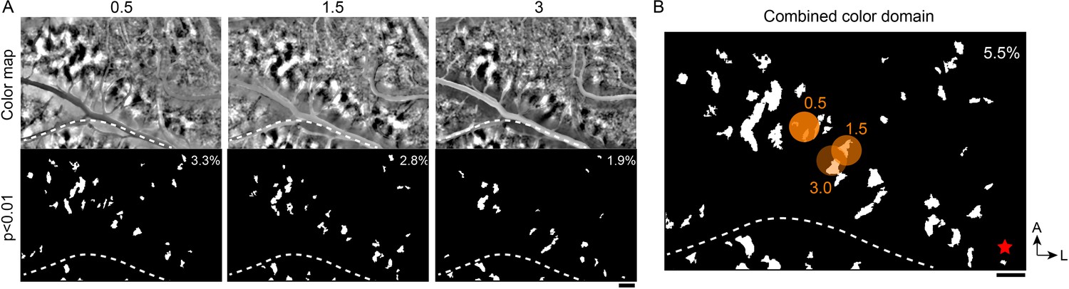
Another example of V4 color map acquired with different spatial frequencies (SFs).
(A) Color maps and corresponding activated regions with different SFs. Top panel: differential maps in response to R/G gratings (corresponding to the black patches) versus W/B gratings (corresponding to the white patches); bottom panel: activated regions by the stimuli, only including color pixels (show significantly stronger responses to R/G gratings, two-tailed t-test, p<0.01). (B) Combined results from (A). Pixels in (A) are superimposed. Numbers in the upper-right corner represent the coverage ratio of activated color domains in V4. Orange dots: centers of activated color domains corresponding to different SFs. Red star: estimated foveal location. Scale bar, 1 mm.
Figure 4—figure supplement 3
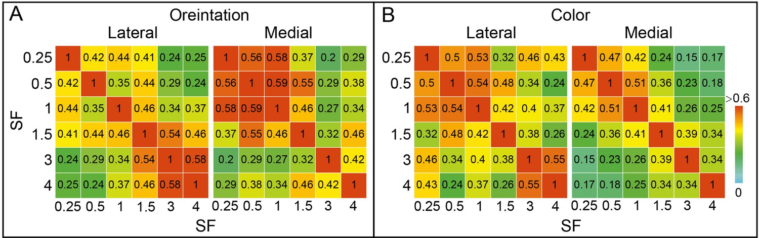
The matrices show the correlation values for pairs of maps acquired with different spatial frequencies (SFs).
Same case as in Figure 4. (A) Matrices of correlation values of orientation maps. (B) Matrices of correlation values of color maps. The imaged V4 regions were divided into two halves: the left half of the region was designated as lateral, the right half was designated as medial, and the correlation value for each half was calculated separately.
Figure 5 with 1 supplement
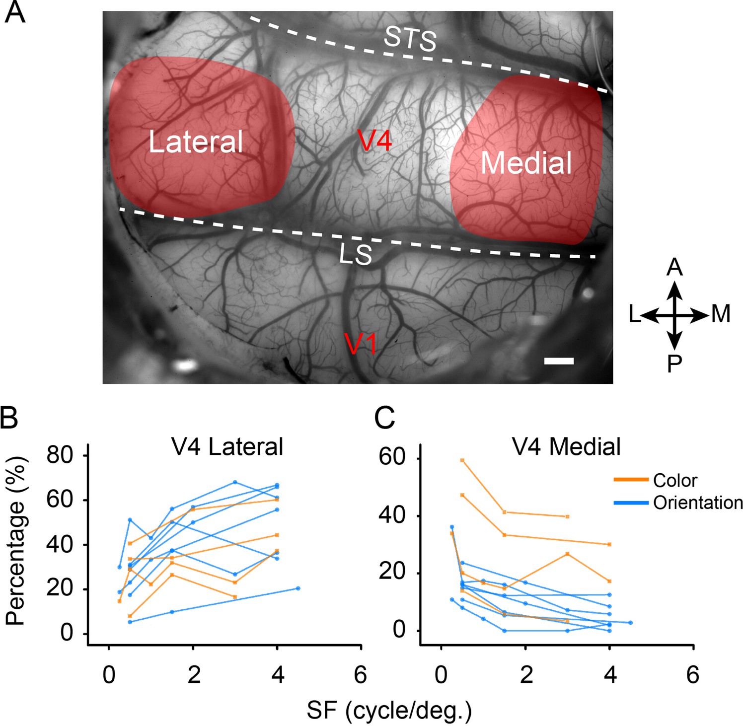
The percentage of selectively activated domains change according to spatial frequency (SF).
(A) Demonstration of cortical blood vessel map and the visual areas chosen for analysis. See Figure 5—figure supplement 1 for details. Scale bar, 1 mm. (B, C) The proportions of activated functional domains in the lateral and medial parts of V4 (color: orange, from four experiments in three hemispheres; orientation: blue, from seven experiments in five hemispheres) change according to SFs. Points connected by a line represent results from the same experiment.
Figure 5—figure supplement 1
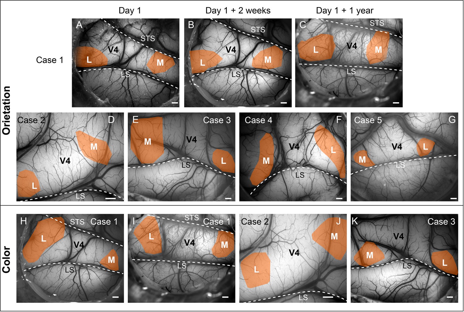
Cortical blood vessel maps of all cases and the corresponding chosen areas for activated percentage analysis in V4.
Orange area: the chosen lateral and medial parts of V4, as mentioned in Figure 5D and E. L: lateral area (foveal area); M: medial area (parafoveal area). LS: lunate sulcus; STS: superior temporal sulcus. (A–G) Chosen area for activated orientation domains from seven experiments in five hemispheres. (H–K) Chosen area for activated color domains from four experiments in three hemispheres. The scale bars in all panels are 1 mm.
Figure 6 with 2 supplements
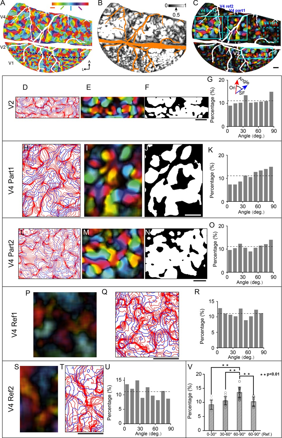
Relationship between spatial frequency (SF) and orientation maps in V4 and V2.
(A) Orientation preference map. Different colors represent different orientation preferences. (B) Orientation selectivity map. The gray scale represents the normalized orientation selectivity (0: no orientation selectivity; 1: strong specific selectivity to one single orientation). (C) Selectivity thresholded orientation preference map (combined result from A and B). Cyan boxes indicate the chosen regions for intersection angle distribution analysis: one V2 region (D–G), two V4 regions (region 1: H–K; region 2: L–O), and two V4 reference regions with weak orientation selectivity (dotted box, V4 Ref1: P–R; V4 Ref2: S–U). (D, H, L, Q, T) Iso-orientation (red lines) and Iso-SF gradient contours (blue lines). (E, I, M, P, S) Selectivity thresholded orientation preference maps corresponding to (D, H, L, Q, T). (F, J, N) Regions (white parts) with high orientation selectivity (normalized orientation selectivity > 0.5) selected for calculating the intersection angle. (G, K, O, R, U) Distributions of intersection angles of the selected regions. The dashed lines indicate the expected value (11.1%) if angles are distributed randomly. (V) Percentage comparison (Wilcoxon rank-sum test) among different angle groups (0–30°, 30–60°, and 60–90° of strong orientation-selective regions, n=15, and 60–90° of weak orientation-selective regions: 60–90° [“Ref.”], n=6). Error bar: SD. Scale bars: 1 mm.
Figure 6—figure supplement 1
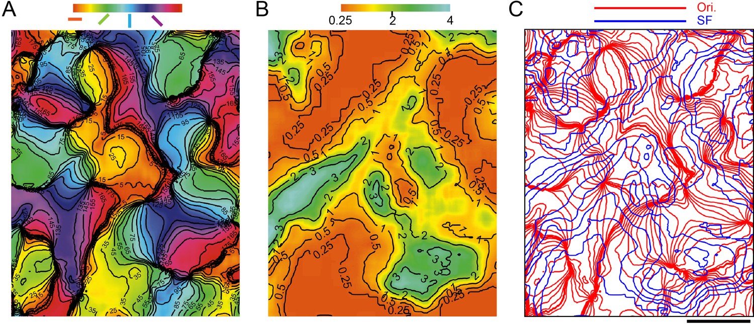
Demonstration of intersections of iso-contour lines for orientation and spatial frequency (SF) maps.
Data from the same case shown in Figure 6, V4 part 1. (A) Iso-orientation gradient lines and orientation preference map. The values indicate the different iso-orientation gradient contours (5°, 15°, 25°, 35°, 45°, 55°, 65°, 75°, 85°, 95°, 105°, 115°, 125°, 135°, 145°, 155°, 165°, 175°). (B) Iso-SF gradient lines (0.25, 0.5, 1, 2, 3 cycles/deg) and SF preference map. (C) Iso-orientation (red lines) and iso-SF gradient contours (blue lines). Scale bar, 1 mm.
Figure 6—figure supplement 2
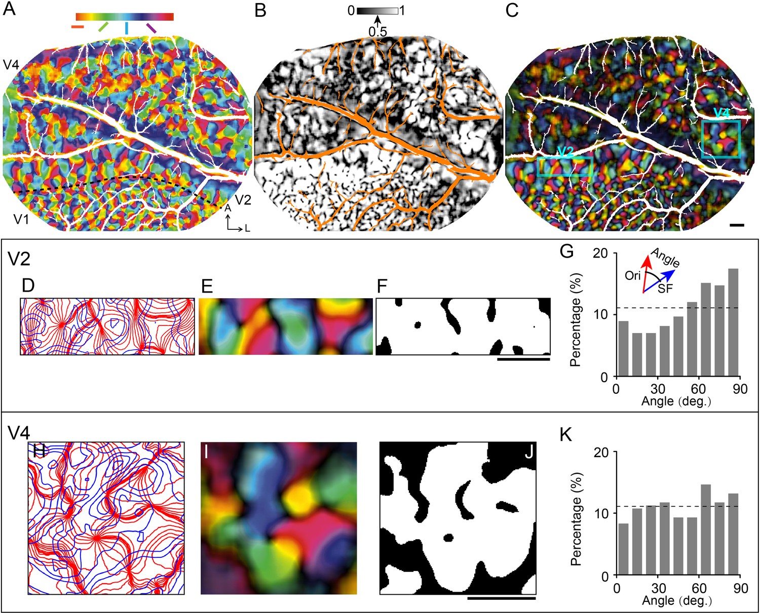
The second case of the relationship between spatial frequency (SF) and orientation maps in V4 and V2.
(A) Orientation preference maps. (B) Orientation selectivity map. The gray scale represents the normalized orientation selectivity. (C) Orientation preference-selective map. The white region in (A) and (C), and the orange region in (B): blood vessels in the cortical surface. One V2 region (D–G) and one V4 region (H–K) were chosen for intersection angle distribution analysis. (D, H) Iso-orientation (red lines) and iso-SF gradient contours (blue lines). (E, I) Enlarged view of orientation preference-selective map in (C) corresponding to (D, H). (F, J) Regions (white regions) with high orientation selectivity (normalized orientation selectivity > 0.5) for calculating the intersection angle. (G, K) Distributions of intersection angles of the selected regions. Dashed lines indicate the expected value (11.1%) if angles are distributed randomly. Scale bars, 1 mm.
Figure 7 with 2 supplements
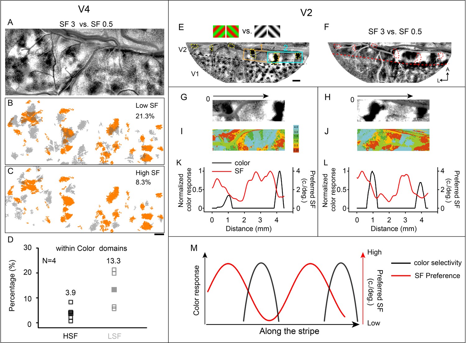
Relationship between spatial frequency (SF) and color-selective domains.
(A–D) Relationship in V4 that high SF domains tend to avoid color domains. (A) Same case as in Figure 4A. Differential SF map in V4 is produced by subtracting the average image of two oriented grating stimuli at a low SF (0.5 cycles/deg) from the corresponding average image at a high SF (3 cycles/deg). The dark patches correspond to regions that prefer higher SF, while the white patches prefer lower SF. (B, C) Overlay of color domains (orange) and SF domains (gray). (B) Low SF domains; (C) high SF domains. Scale bar, 1 mm. (D) The percentage of HSF/LSF (high spatial frequency/low spatial frequency) selectivity regions within color domains was calculated. Unfilled squares represent the results from each case (four cases). Filled squares are the averaged outcomes from the four cases. The mean value is shown on top of the corresponding group. For the other three cases, see Figure 7—figure supplement 1. (E–M) Relationship in V2 that stripe-like distribution of SF preference changes periodically. Data from the same case shown in Figure 3, case 1. (E) Color map. Regions 1 (orange rectangle) and 2 (cyan rectangle) were selected for further analysis in (G–L). In V2, the yellow dashed outlines highlight the color domains. The border between V1 and V2 is indicated by a black dashed line. Scale bar, 1 mm. (F) Differential SF maps produced by subtracting the average image of two oriented grating stimuli at a low SF (0.5 cycles/deg) from the corresponding average image at a high SF (3 cycles/deg). Red dashed outlines: color domains same with those in (E). (G, H) Enlarged color maps from regions 1 and 2. (I, J) Enlarged SF maps from regions 1 and 2. (K, L) Changes of color-selective response (black lines) and SF preference (red lines) along the path parallel to V1/V2 border in V2. (M) Similar to color selective responses in V2, SF preference changes along V1/V2 border.
Figure 7—figure supplement 1
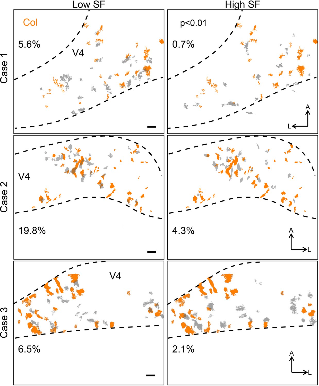
Relationships between V4 spatial frequency (SF) and color-selective domains in three cases.
SF domains (marked by gray) were the areas with a significant response difference (two-tailed t-test, p<0.01) between low SF conditions (0.25–0.5 cycles/deg, 45° and 135°, left panel) and high SF conditions (3–6 cycles/deg, 45° and 135°, right panel). Color domains (marked by orange) were superimposed over results based on activated regions (in gray) under different SF conditions. Each row of subplots represents results from different cases. Scale bar: 1 mm.
Figure 7—figure supplement 2
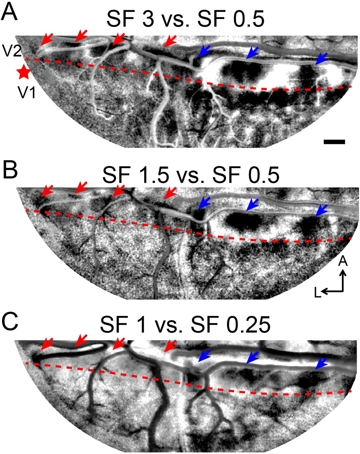
Differential spatial frequency (SF) maps acquired by subtractions between different SF pairs (same case as Figure 7).
(A–C) Differential SF maps produced by subtracting the average image of two oriented grating stimuli at a low SF (A, B: 0.5 cycles/deg; C: 0.25 cycles/deg) from the corresponding average image at a higher SF (A: 3 cycles/deg; B: 1.5 cycles/deg; C: 1 cycle/deg). Red star: estimated foveal location. The arrows indicate the high SF preference regions in V2. Scale bar: 1 mm.
Author response image 1
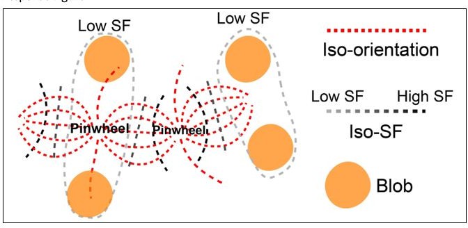
Illustration of the architecture in V1.
Some of the pinwheel centers are in low SF, and some are in high SF. The iso-SF contours (achromatic dashed lines) intersect with iso-orientation contours (red lines connecting two neighboring pinwheel centers) mostly at a right angle. Low SF preference regions (circled by light gray dashed lines) are filled with orientation domains that prefer low SF and color blobs (orange patches).
Author response image 2

Color maps obtained by comparing red/green and white/black gratings with different orientations.
A. Used orientations: 45° and 135°. B. Used orientations: 45°. C. Used orientations: 135°.
Tables
Table 1
Summary of the preferred spatial frequencies (SFs) in different visual areas.
| Preferred SF (mean ± SD cycles/deg.) | V1 | V2 | V4 |
|---|---|---|---|
| Case 1 | 2.86 ± 1.40 N = 147,207 | 2.03 ± 1.51 N = 103,377 | 1.23 ± 1.32 N = 490,921 |
| Case 2 | 2.96 ± 1.37 N = 194,847 | 2.20 ± 1.52 N = 186,288 | 1.15 ± 1.26 N = 635,679 |
Table 2
Comparisons used to generate different functional domains.
| Comparison | Domain type | ΔdR/R criteria |
|---|---|---|
| RG vs. WB | Color | <0 |
| Luminance | >0 | |
| 0° vs. 90° | 0° | <0 |
| 90° | >0 | |
| 45° vs. 135° | 45° | <0 |
| 135° | >0 | |
| High SF (≥2 cycles/deg) vs. low SF (<1.5 cycles/deg) | High SF | <0 |
| Low SF | >0 |
-
SF: spatial frequency.
Additional files
Download links
A two-part list of links to download the article, or parts of the article, in various formats.
Downloads (link to download the article as PDF)
Open citations (links to open the citations from this article in various online reference manager services)
Cite this article (links to download the citations from this article in formats compatible with various reference manager tools)
Spatial frequency representation in V2 and V4 of macaque monkey
eLife 12:e81794.
https://doi.org/10.7554/eLife.81794


