Figures and data in Oligodendrocyte-mediated myelin plasticity and its role in neural synchronization

Figures
Tables
Additional files

4 figures, 5 tables and 1 additional file

Figures

Figure 1 with 4 supplements

Download asset Open asset

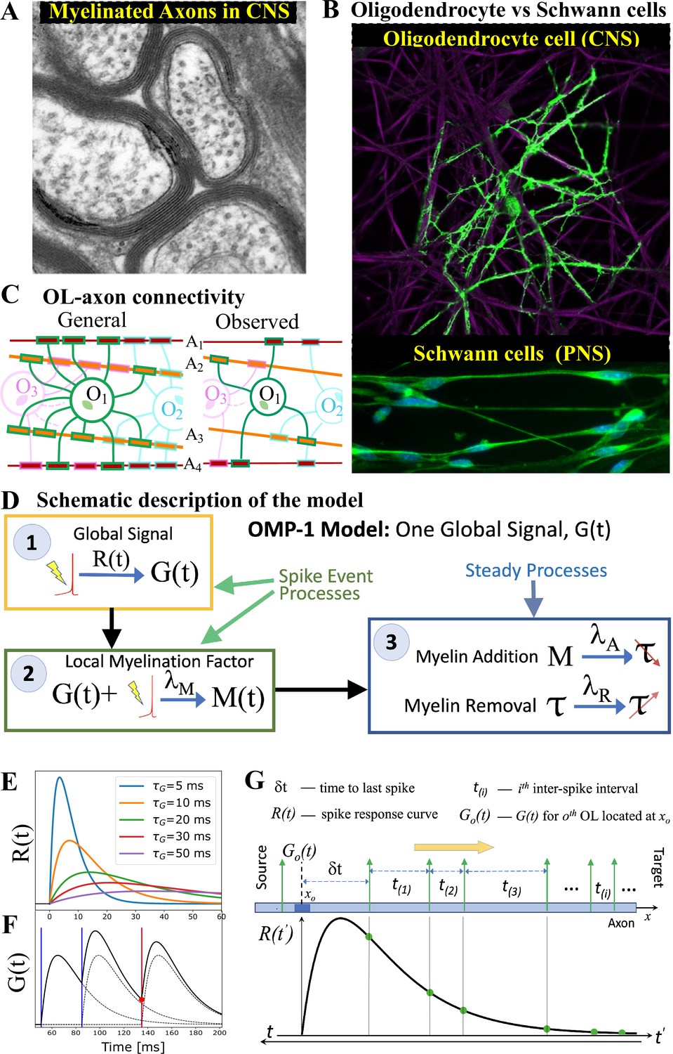
OMP motivation and model description.

(A) Cross-section of myelinated axon bundle in CNS illustrates that myelin thickness on adjacent axons differs. (B) Single OL (green) myelinates many different axons (purple), which is in stark contrast to Schwann cells in the PNS, which myelinate only one axon. (C) OL-axon connectivity: OLs tend to avoid placing multiple processes on a single axon, thus maximizing the number of axons it myelinates. (D) Schematic depiction of the OMP-1 model which contains only the three basic steps required for this type of OMP to work. (E) Spike-response curves $R (t)$ for increasing values of $τ_{G}$ . (F) The equation governing the release of $G (t)$ is linear and the response to multiple spikes (vertical lines), is the linear sum of individual responses (dashed lines). The release of $M$ after each spike at any given OL process/axon will be proportional to the amplitude of $G (t)$ at the time of spike (red dot for red spike). (G) The sum over responses can also be viewed as sampling of $R (t)$ in reverse time. Panels A and B have been adapted from Chapter 45 Figure 1 in Fields, 2013, used with permission.

Figure 1—figure supplement 1

Download asset Open asset

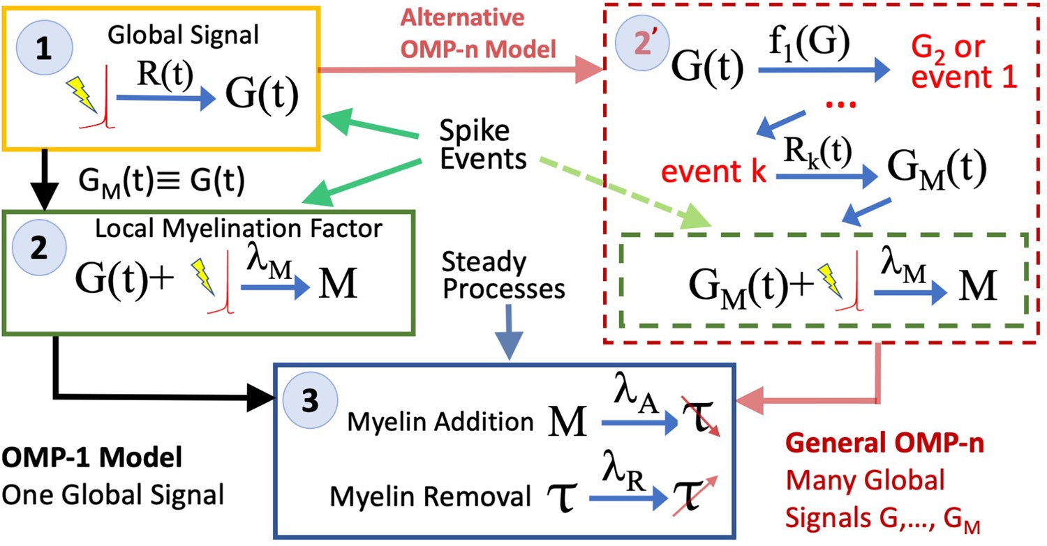
OMP-1 model vs OMP-n model.

A more complex OMP models can be constructed; however their structure differs from the simplest OMP-1 model only in step 2, where multiple global factors can participate, together with a cascade of events, which can be triggered by given threshold events, each potential having their own response functions, $R_{k} (t)$ . Ultimately, the whole cascade will lead to the production of the myelination-promoting factor $M$ , as in the case of OMP-1.

Figure 1—figure supplement 2

Download asset Open asset

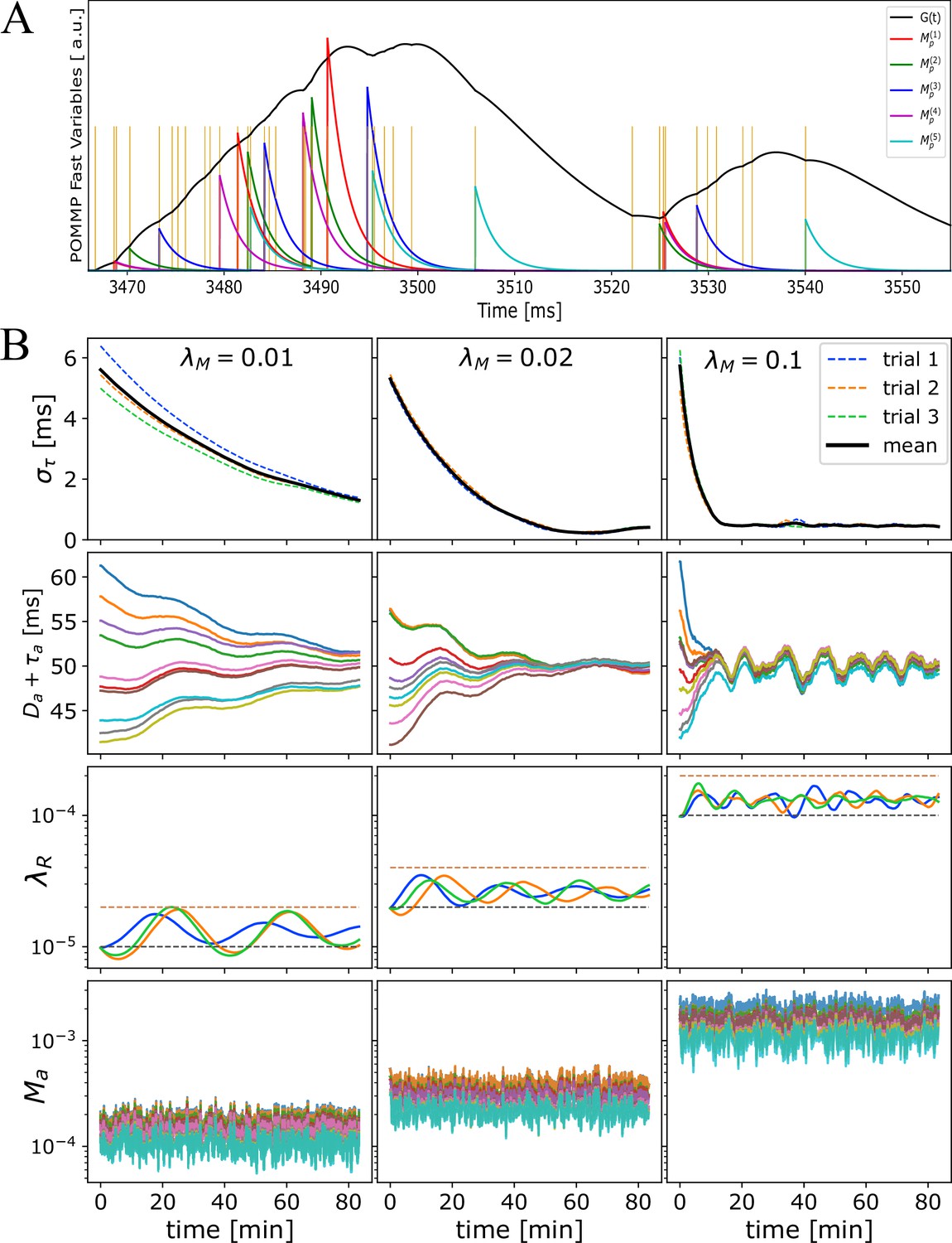
Time progression of OMP fast and slow variables.

Time progression of OMP variables when correlated Poisson spikes are conducted through OC with a single OL, $N_{O} = 1$ , and for $N_{A} = 10$ axons. The ordering of the spikes carries statistically the signature of the fixed delays. The OMP parameters for this simulation are $τ_{G} = 30$ ms, $τ_{s} = 100$ ms, $λ_{A} = 0.1$ ms^-1, $σ_{j} = 5$ ms, $λ_{M} = 0.01$ ms^-1, and $λ_{H} = 10^{- 6}$ ms^-1. (A) A millisecond time-scale dynamics of $G (t)$ and $M_{a} (t)$ , in response to incoming spikes (yellow vertical lines). For clarity, only five of the total $N_{A} = 10$ axons are shown. Time reported in milliseconds is just an offset from the beginning of the last $T_{e} = 10$ second epoch. (B) Time progression of $σ_{τ}$ (top row) and OMP model variables, as indicated, over $T_{\exp} = 5000$ seconds, plotted as the averages over $T_{e} = 10$ second epochs, and different columns showing different values of $λ_{M}$ , as indicated. The second row from the top shows the 10 delays for each axon, for a single trial, combined with the fixed delays (showing the convergence of the arrival times). The third row shows the time evolution of the myelin removal rate, $λ_{R}$ , guided by the homeostatic equation (Equation 17) with black and red dashed lines indicating the simple homeostatic balance estimate ( $λ_{M} N_{A} / τ_{s}^{2}$ ) and twice that value, respectively. Differently colored trajectories are the results from three independent trials, with the same parameters but different random initializations of fixed and adaptive delays ( $σ_{D} = 5$ ms). The bottom row shows the concentrations of $M$ for each axon in a single trial. For the relatively large, $τ_{G} =$ 30 ms, differences in concentrations are not as drastic as they are for $τ_{G} =$ 10 ms (see Figure 2—figure supplement 1).

Figure 1—figure supplement 3

Download asset Open asset

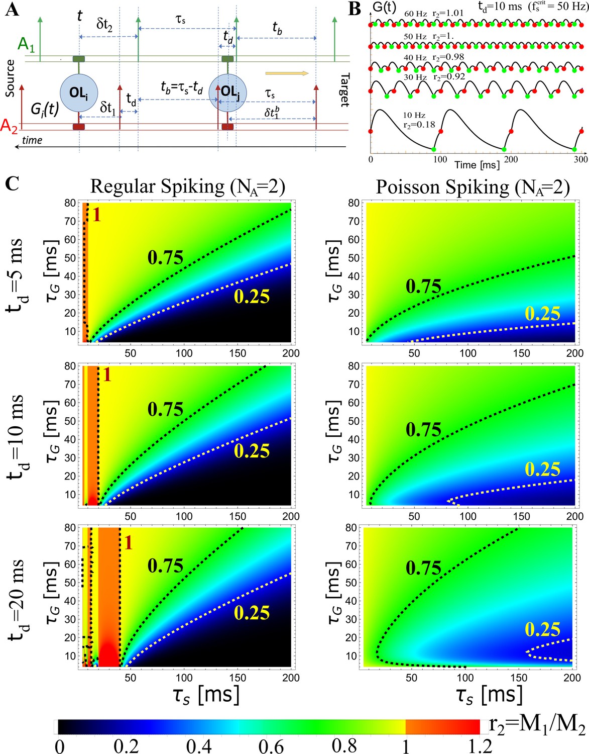
Theoretical predictions of OMP model.

Theoretical predictions for $M_{a}$ for $σ_{j} = 0, N_{A} = 2$ . (A) Schematic depiction of the temporal relationship between spikes in a pair of axons ( $A_{1}, A_{2}$ ; $N_{A} = 2$ ) in the case of regular spiking, illustrating different scenarios when calculating $G (t)$ . The ‘leading’ edge spikes (green) are offset by a fixed delay, t_d, over the ‘lagging’ spikes (red). (B) Examples of $G (t)$ for $t_{d} = 10$ ms and for five different spiking frequencies $f_{s} \in [10, 30, 40, 50, 60]$ Hz, as indicated, showing also the corresponding ratios, $r_{2} = M_{1} / M_{2} = M_{g r e e n} / M_{r e d}$ . Occurrences of ‘red’ and ‘green’ spikes are plotted together with $G (t)$ , indicating also the level of $M$ released, as it is proportional to $G (t)$ . We see that up to the critical frequency, $f_{s}^{c r i t} = 50$ Hz, the lagging axon will have more myelination factor, $M$ , as desired, but this reverses above the critical frequency. (C) Theoretical predictions for the ratio, $r_{2} = ⟨ M_{1} ⟩ ⟨ M_{2} ⟩ .$ , as a function of $τ_{G}$ and $τ_{s}$ for three different fixed time-delays, $t_{d} =$ 5, 10, and 20 ms (rows, as indicated), in the case of regular (left column) and Poisson (right column) spiking. The regions with red/orange hues are the regions of instability, where, $r_{2} > 1$ which will lead to further desynchronization, and is only happening for regular spiking. For Poisson spiking, the ratio is always lt₁, as is evident from Equation 3, hence, the ‘lagging’ axon will always have enhanced myelination relative to the ‘leading’ axon, due to a higher concentration of, $M$ which is desired for stable synchronization in all regimes.

Figure 1—figure supplement 4

Download asset Open asset

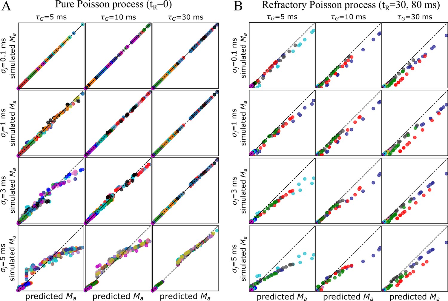
Theoretical predictions vs simulations.

Comparing theoretical predictions with simulations ( $σ_{j} > 0, N_{A} = 10$ ). The mean $M_{a}$ values obtained in simulations (y-axis) are compared to the theoretical prediction (x-axis) given by Equation 4, which ignores jitter. (A) The mean $M_{a}$ values are from a simulation sets specified in Appendix 1—table 4, for which correlated Poisson spiking was used. The results are shown as a grid plot for different values of jitter and characteristic spike response time, $τ_{G}$ . Individual points from the same parameter set are colored the same, with different parameter sets/runs being colored by cycling through 15 different colors with no particular meaning attached to the coloration. Each set had 2, 5, or 10 points (one per axon). We see that the predictions made for $σ_{j} = 0$ case hold very well for small jitter ( $\leq σ_{j} \leq 1$ ), but fail for larger jitters, particularly for $σ_{j} = 5$ ms, making the differences in $M_{a}$ across axons smaller. Nevertheless, even for large jitter, when $τ_{G}$ is large enough, the prediction given by Equation 4 is in reasonable agreement with the observed/simulated values. (B) Same as in (A), but this time spikes were simulated using a refractory Poisson process with $t_{R} = 30$ and $t_{R} = 80$ ms. Because now it violates the assumption of a memoryless process, under which the derivation of Equation 4 is made, the predictions fail for any amount of jitter or $τ_{G}$ . We note that theoretical predictions for a general renewal process with any amount of jitter are outside the scope of the current manuscript.

Figure 2 with 2 supplements

Download asset Open asset

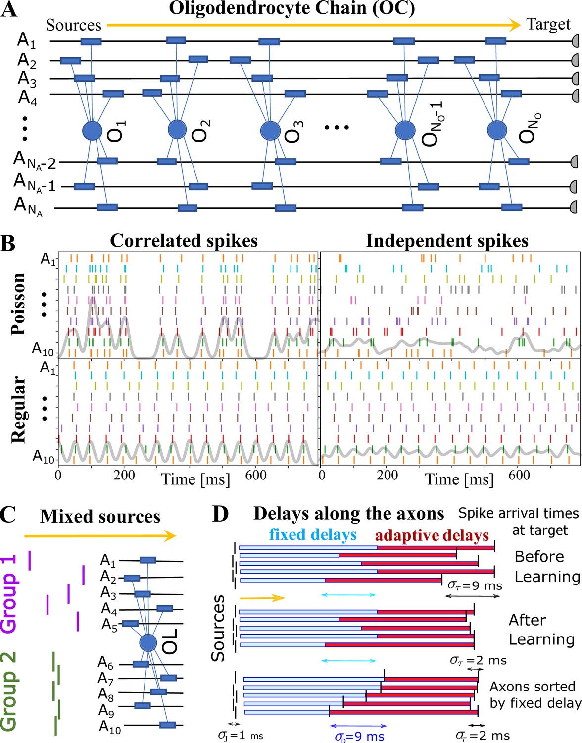
OMP simulations with action potentials/spikes conducted along ‘oligodendrocyte’ chain (OC).

(A) OC with $N_{O}$ ‘effective oligodendrocytes’ (segments), myelinating $N_{A}$ axons ( $ℳ$ is an $N_{O} \times N_{A}$ matrix of ones). (B) examples of ‘pure’ spikes used in our simulations: correlated *versus* independent spikes, and Poisson *versus* regular spiking. Gray lines are moving averages of all spikes using a sliding Gaussian window with 10 ms RMS width. (C) example of ‘mixed’ signals in which axons in Group 1 are conducting independent spikes and those in Group 2 carry correlated spikes. The two groups can potentially interfere with the expected synchronization behavior of each ‘pure’ group. Different groups could also contain spikes time-locked within each group, but independent between the groups. (D) schematic depiction of time delays between the signal source and the target. Fixed delays are not modifiable and essentially represent the spread in spike times as they enter the axonal bundle of myelinated axons, whose delays are adaptive. Note, that the horizontal bars represent the magnitude of the fixed and adaptive delays, not the axons.

Figure 2—figure supplement 1

Download asset Open asset

Time progression of OMP variables for correlated spikes.

Time progression of the slow variables in the OMP model, similar to one shown in Figure 1—figure supplement 2B, but now with faster spike responses in the OL, $τ_{G} = 10$ ms, and for different $λ_{H}$ (values shown in columns), using only one myelin production rate, $λ_{M} = 0.02$ , and $σ_{j} = 1$ ms. The independent trials, each have with their own set of randomly chosen fixed delays ( $σ_{D} = 6$ ms). The top row shows the time progression of $σ_{τ}$ for each trial (dotted red line is the mean over all trials). The second row are the 10 delays, $τ_{a}$ , for each axon, and the third row are the same delays when combined with the fixed delays (showing the convergence of the arrival times). The fourth row shows the time evolution of $λ_{R}$ , with black and red dashed lines indicating values $λ_{M} N_{A} / τ_{s}^{2}$ (the balancing estimate for independent spikes) and twice that value, respectively. The bottom row shows the concentrations of $M$ for each axon.

Figure 2—figure supplement 2

Download asset Open asset

Time progression of OMP variables for independent spikes.

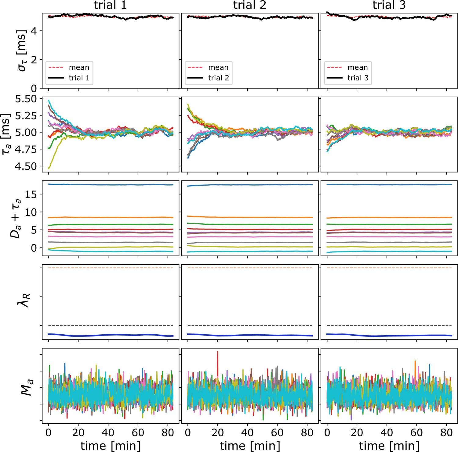
Time progression of the slow variables (averages over $T_{e} = 10$ s epochs) in the OMP model when the spikes are independent with Poisson ISI. Here, the columns show three independent trials with the same set of OMP parameters but each with its own set of randomly chosen fixed delays ( $σ_{D} = 5$ ms). The OMP parameters for this simulation are $τ_{G} = 10$ ms, $τ_{s} = 100$ ms, $λ_{M} = 0.01$ , $λ_{H} = 10^{- 7}$ $σ_{j} = 1$ ms, $N_{O} = 10$ and $N_{A} = 10$ axons. The top row shows the time progression of $σ_{τ}$ for each trial (dotted red line is the mean over all trials). The second row are the 10 axonal delays, $τ_{a}$ and the third row are the same delays when combined with the fixed delays (showing the delay profile that will be fed into the next OL segment in the chain). The fourth row shows the time evolution of $λ_{R}$ , with black and red dashed lines indicating values $λ_{M} N_{A} / τ_{s}^{2}$ (the balancing estimate for independent spikes) and twice that value, respectively. The bottom row displays the concentrations of $M$ for each axon.

Figure 3 with 2 supplements

Download asset Open asset

OMP model behavior as a function of OMP and signal parameters.

(A) When spikes are independent, $σ_{τ} (t)$ consistently show no change in overall synchronization (purple; innermost circle in the model selection pie-chart); for correlated signals significant synchronization occurs, largely depending on $τ_{s}$ and $τ_{G}$ . (B) individual OMP synchronization profiles, $σ_{τ} (t)$ , simulations for $N_{A} = 10$ , $λ_{H} = 10^{- 6}$ , $λ_{M} = 0.02$ , with $τ_{G} = 30$ ms (top panel) vs. $τ_{G} = 10$ ms (bottom). Dashed lines are for $N_{O} = 1$ and solid lines for $N_{O} = 10$ . Colors indicate the jitter level: $σ_{j} = 1$ ms (red), $σ_{j} = 3$ ms (blue), $σ_{j} = 5$ ms (green). (C) dependence of $σ_{τ} (t)$ on the number of OLs, $N_{O}$ , in the OC. We show both the comparison based on the raw time, as well as when matched in terms of the total number of neural spikes encountered by the OLs (inset). (D) density of $σ_{τ}^{\infty}$ estimates dependence of $σ_{τ}$ on the number of OL in OC. (E) Percent reduction in $σ_{τ}$ vs $τ_{G}$ and $τ_{s}$ for $σ_{D} = 10$ ms; (inset) ratio of the $M$ concentrations for two axon case, $N_{A} = 2$ , which matches well the overall pattern of synchronization. (F) dependence of $σ_{τ}^{\infty}$ (bar plot) and the synchronization time constant, $τ_{L} = 1 / L_{τ}$ , (semi-log plot, above) on the number of axons, $N_{A}$ values are only for runs declared as E1 blue curve inset indicates percent of E1, for different $N_{A}$ (for all spike rates).

Figure 3—figure supplement 1

Download asset Open asset

Exploring OMP properties and parameters.

Exploring OMP with a large number of parameter settings. (A) For any given setting of OMP parameters, simulations are repeated n_r times each with a random choice of fixed delays ( $D_{a}$ , parameterized with $σ_{D}$ ) and initial adaptive delays (parameterized with $τ_{0}$ and $p_{τ}$ ). These individual temporal profiles/trials (colored lines) are averaged and the mean is reported as the synchronization profile, $σ_{τ} (t)$ (that we refer to as a set or run). (B) A grid plot of $σ_{τ} (t)$ for correlated spikes using 12 parameter runs (3 trials and the mean), revealing its dependence on $N_{O}$ and $σ_{j}$ (4 $N_{O}$ and 3 $σ_{j}$ values, for $N_{A}$ = 10, $τ_{G} = 10$ ms, $λ_{H} = 0.000001$ , $λ_{M} = 0.02$ ). Some of these profiles are shown in Figure 3B to illustrate OMP instabilities with small $N_{O}$ and fixed delays, which are overcome with increasing $σ_{j}$ and $N_{O}$ . (C) The center panel shows all runs specified in the left panel of Appendix 1—table 1. We summarize such large number of runs in two ways: (1) we average all $σ_{τ} (t)$ within a subset of runs grouped by some parameter, $τ_{G}$ , as shown in the left panel; (2) we also fit all $σ_{τ} (t)$ to 5 models, as described in Materials and Methods, and plot the distribution of $σ_{τ}^{\infty}$ as shown in the right panel. In some cases we also plot the distribution of $τ_{L}$ parameters. (D) Figure 3A results with $σ_{D} = 10$ ms are shown here for $σ_{D} = 5$ ms and also (E) compared to the equivalent runs using the instantaneous myelination OMP model. We used a smaller bandwidth for kernel density estimation to highlight the differences, which are not apparent at smoother KDE values. (F) Summary of average profiles grouped by $N_{A}$ , shown in Figure 3F for $σ_{D} = 5$ ms, and additionally for $σ_{D} = 10$ ms.

Figure 3—figure supplement 2

Download asset Open asset

Model fitting for synchronization profiles.

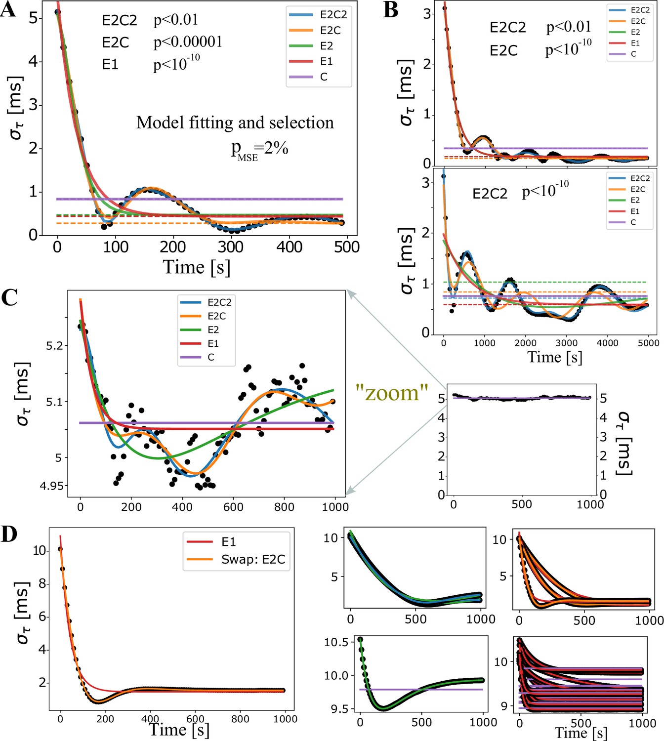
Model fits for quantifying synchronization performance across different parameter runs.

(A) An example of fits for all five nested models. Dashed lines represent estimates of the long-time baseline, $σ_{τ}^{\infty}$ . (B) In most cases, comparing the dashed lines, the model selection does not affect the estimate of the baseline (top panel), but can sometimes have a significant impact. For example, in the bottom panel, the baselines differ by nearly 50%. For such a complex synchronization profile it is actually hard to determine the true long-time baseline and the only way to resolve those situations is to run really long simulations, which we could not afford in this early and extensive exploratory phase. (C) In the majority of runs, the less restricted models were deemed the best with the standard F-test. When magnified, it is clear that E2C2 offers a statistically better description than the constant model, which we label (C). On the other hand, when considered at the full scale (small graph on the right), we desire to classify such a profile simply as the constant model, (C). This is achieved by introducing a fudge factor, $p_{MSE} = 2$ %, which under our modified F-test selects the model C. (D) We also introduced a ‘swapping’ rule. This rule reverts the fit back to the less restricted model when the true MSE in the restricted model is 500 times larger than the one for the restricted model. This did not seem to be consequential, as in most simulations very few swaps occurred, and when they occurred seemed to be justified, as shown in the large panel on the left, where the E1 model suggestion, given by the modified F-test, was reverted to a double exponential fit. The four panels on the right show all swaps obtained with runs specified in Oligodendrocyte-mediated Myelin Plasticity and its Role in Neural Synchronization Appendix 1—table 3, which was the case that had most of the swaps, and most of those were swaps from C to E1 (lower right panel) which had a very small range. Hence, the swap did not change $σ_{τ}^{\infty}$ significantly but had a large effect on the value of $τ_{L}$ , which is hence less reliable in our summary statistics.

Figure 4 with 3 supplements

Download asset Open asset

Selective synchronization with mixed signals; effects of $λ_{H}$ and $σ_{D}$ parameters.

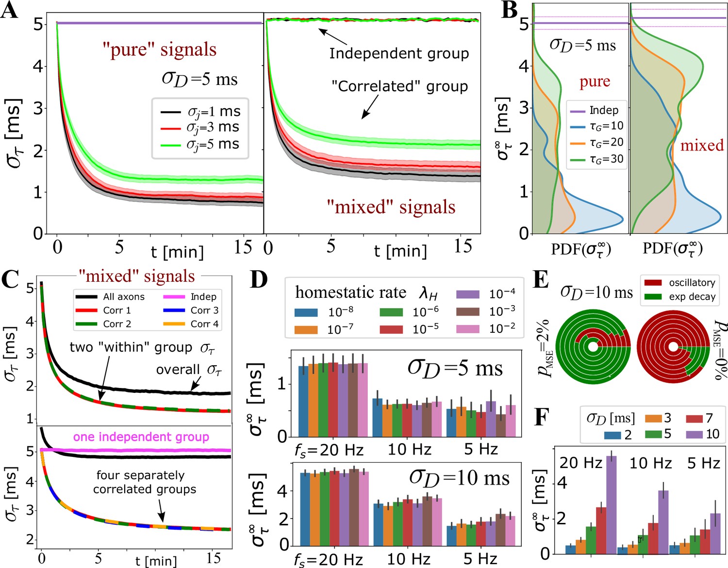
(A) Average $σ_{τ} (t)$ (grouped by $σ_{j}$ ; shaded regions indicate SE over the parameter sets for $N_{A} = 10$ and $σ_{D} = 5$ ; see Appendix 1—table 2). In the left panel is the average for the set of $N_{A} = 10$ axons conducting only ‘pure’ correlated signals, and on the right are the averages within two groups of 10 axons, out of $N_{A} = 20$ total that OL myelinates, carrying ‘mixed’ signals – one group conducting correlated signals and the other independent signals. The behavior of the correlated groups is clearly distinguishable from the independent ones (indicated by arrows). (B) Estimated density for $σ_{τ}^{\infty}$ comparing pure (left) vs mixed signals (right panel) for a wider range of parameters, including $N_{A} = 20$ and $N_{A} = 50$ , but with the number of axons carrying correlated signals matched in all cases ( $N_{A} = 10$ , $N_{A} = 25$ ). (C) Top panel shows $σ_{τ} (t)$ for two groups of correlated signals (colored lines) with Poisson spiking (correlated within group, but mutually independent); bottom panel shows results for four separately correlated groups + 1 independent group (cyan). Black lines represent the spread over all axons. (D) Investigating the influence of homeostatic regulation and homeostatic rate, $λ_{H}$ , grouped by different firing rates and different $σ_{D}$ . (E) Model selection chart depicting the relative proportions of oscillatory (E2C2, E2C) vs stable, single exponential (E1) $σ_{τ} (t)$ , for two different values of the F-test fudge-factor $p_{MSE}$ ; the innermost circle is for $λ_{H} = 10^{- 2}$ and the outermost for $λ_{H} = 10^{- 8}$ . (F) OMP synchronization performance for different magnitudes of fixed delays, $σ_{D}$ .

Figure 4—figure supplement 1

Download asset Open asset

Supplemental results for Figure 4.

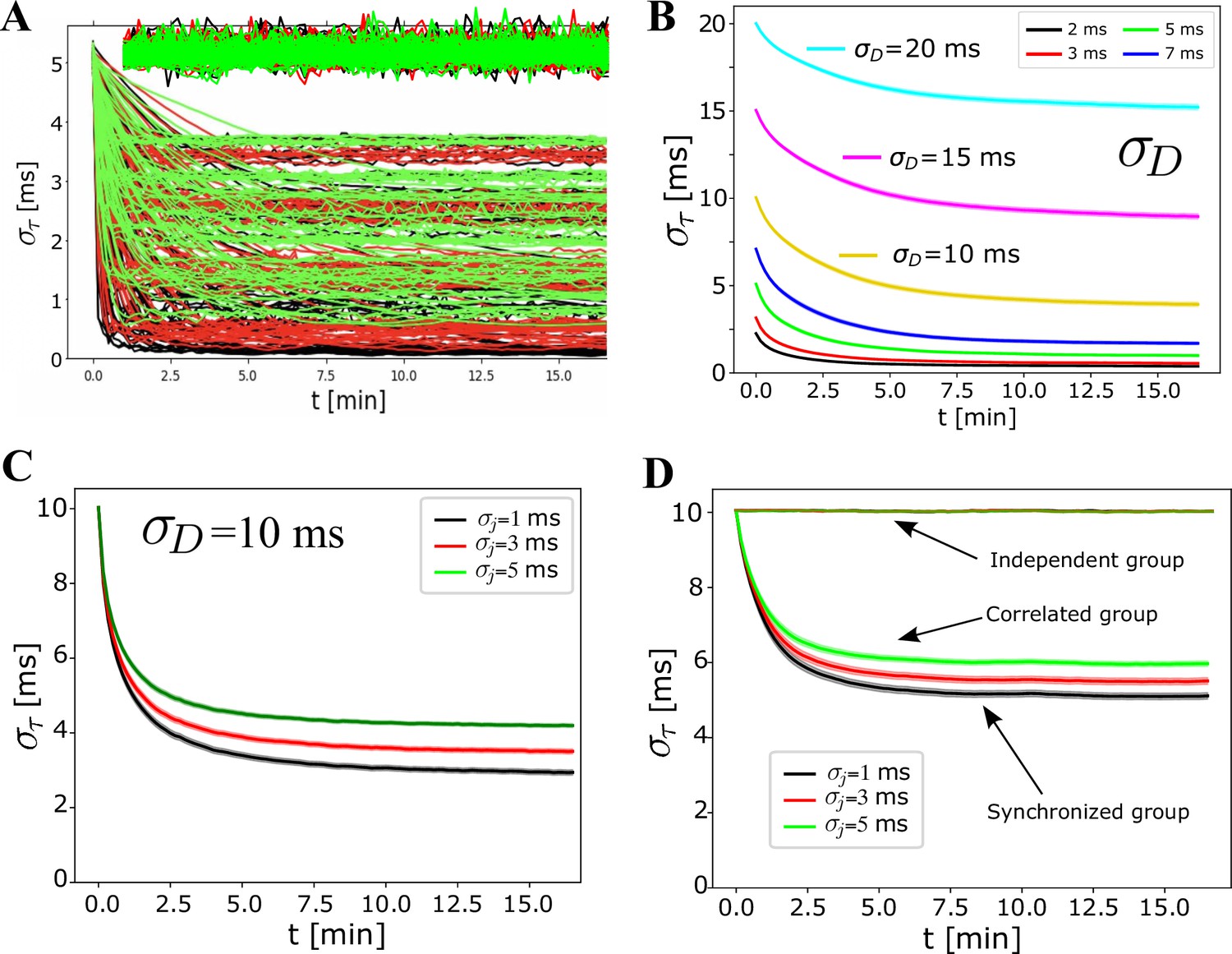
(A) Individual runs for the averages reported in Figure 4A for mixed signals, one conducting correlated spikes and the other independent spikes. Individual runs for independent spikes here are manually offset for clarity, not to overlap with profiles obtained with the correlated spikes, but are mainly shown to demonstrate that the actual spread in the performance is much larger than what the shaded standard error (SE) indicates for the independent group, appearing only as lines when averaging over many runs (and drawn as a ‘thick’ purple line for pure independent signals in Figure 4A, where the SE was even smaller). (B) Influence of $σ_{D}$ on synchronization efficiency. (**C–D**) Averages over all runs with $σ_{D} = 10$ ms, grouped by jitter, comparing (C) pure signals with (D) mixed signals with one independent and one correlated group, as was similarly shown in Figure 4A for $σ_{D} = 5$ ms.

Figure 4—figure supplement 2

Download asset Open asset

Influence of additional OMP and signal parameters.

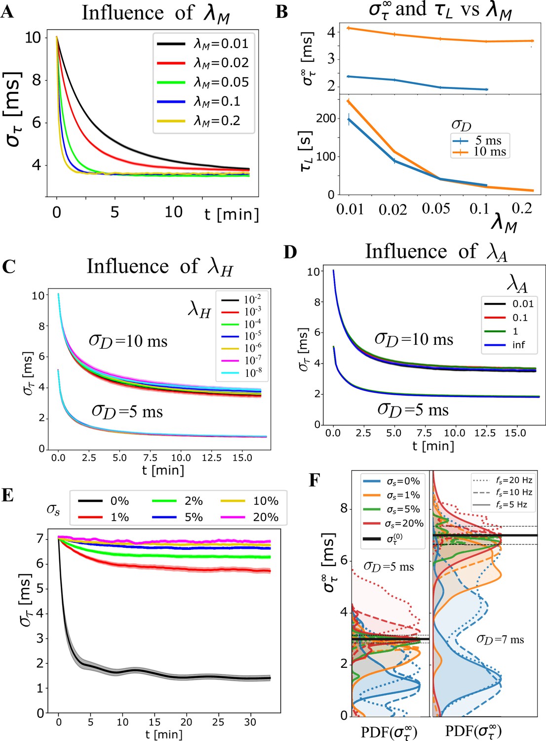
Exploring additional OMP and signal parameters. (A) Average $σ_{τ} (t)$ , grouped by $λ_{M}$ , which highly influences the learning rate, as it sets the time scale for changes in myelination. (B) Bottom panel shows this explicitly via ‘learning time’, $τ_{L} = 1 / L_{τ}$ , as a function of $λ_{M}$ for $σ_{D} =$ 5 and 10 ms. The dependence of $σ_{τ}^{\infty}$ on $λ_{M}$ (top panel) was not strong and it appears to slightly favor faster rates. This ‘slight’ trend does not appear consistently and depends on the range of parameters chosen for averaging. (C) The average $σ_{τ} (t)$ for $σ_{D} = 10$ and $σ_{D} = 5$ ms, respectively, show that $λ_{H}$ does not have a strong influence on the behavior of the OMP model (also emphasized in Figure 4E). (D) Average $σ_{τ} (t)$ for $σ_{D} = 10$ and $σ_{D} = 5$ ms now grouped by the myelin conversion rate, $λ_{A}$ , including the instantaneous myelination model, Equation 15, and showing that $λ_{A}$ has a very small influence on synchronization. This might change when the saturation limits $τ_{\min}$ , $τ_{\max}$ become narrower, as well when different $τ_{nom}$ values in Equation 17 are used. We use saturation limits that allow highly heterogeneous values for the delays (3 ms to 100 ms), making it harder to achieve synchronization. (E) The sensitivity of OMP to firing rate variability, specified via $σ_{s}$ in the case of regular spiking, having ‘beating’ synchronized periods, but also even longer non-synchronized periods, potentially detrimental to the synchrony. Averages, grouped by $σ_{s}$ , indicate that when the spiking-rate variability is smaller than 5%, synchronization still occurs but is very inefficient. This might not be a problem since myelin plasticity operates on a very slow time scale, measured in days and months, but only if $σ_{τ}$ does not get worse during non-synchronized epochs. (F) The sensitivity to $σ_{s}$ quantified via $σ_{τ}^{\infty}$ , showing that variations greater than 5% exhibit de-synchronization effects but these might not arise for Poisson spiking.

Figure 4—figure supplement 3

Download asset Open asset

Oscillations due to homeostatic regulation.

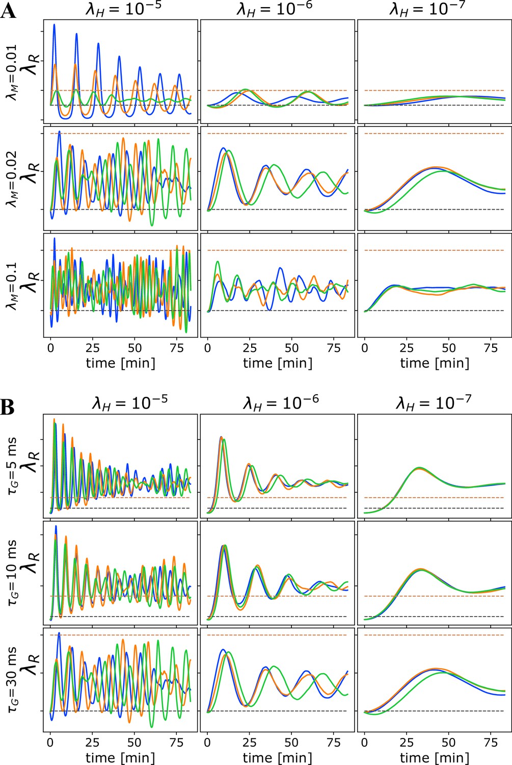
Oscillations in $λ_{R}$ due to homeostatic regulation. The theoretical guess for the balance between addition and removal of myelin, that we initialize $λ_{R}$ to at the start of each simulation, should work well for independent spikes, if saturation effects can be ignored. However, in most cases, this prediction does not match the true balancing value for $λ_{R}$ , and hence for fast homeostatic rates, the approach to equilibrium will be too fast and will induce oscillations. (A) Time progression of $λ_{R}$ in the OMP model for three different values of $λ_{H}$ (columns) and three different values of $λ_{M}$ when a set of correlated spikes with exponential ISI (Poisson) are conducted through = $N_{A}$ 10 axons. For this set of runs $N_{O} = 1$ , $τ_{G} = 30$ , and $σ_{j} = 5$ . (B) Time progression of $λ_{R}$ in the OMP model for three different values of $λ_{H}$ (columns) and three different values of $τ_{G}$ when a set of correlated spikes with exponential ISI (Poisson) are conducted through = $N_{A}$ 10 axons. For this set of runs, $N_{O} = 1$ , $σ_{j} = 5$ and $λ_{M} = 0.02$ . The spike-response time, $τ_{G}$ , does not influence the oscillation frequency of $λ_{R}$ as strongly as $λ_{M}$ .

Tables

Table 1

List of symbols used in the manuscript: OMP model parameters, OMP variables, spiking signal parameters, and data analysis and quantification parameters and other symbols.

For each we provide a short description and the range of the parameter values, or its dimensionality, in the case of the variables.

List of symbols used in this manuscript
Symbol	Description	Explored Values/Dimensionality
OMP model parameters
$R (t)$	OL transient response curve	see $τ_{G}$
$τ_{G}$	characteristic time for $R (t)$ ( $τ_{G} = τ_{r} = τ_{d}$ )	[2-100] ms
$λ_{M}$	production rate for factor $M$	[0.01, 0.5] ms^-1
$λ_{A}$	myelin conversion/addition rate	[0.01, 0.5] ms^-1
$λ_{R}$	myelin removal rate	Equation 16; variable for $λ_{H} > 0$
$λ_{H}$	homeostatic rate	[0, 10^-2] ms^-2
$N_{O}$	number of OL in OC	[1-20]
$N_{A}$	number of axons	[2-150]
$M$	myelination matrix	$N_{O} \times N_{A}$ : {full connectivity}
$τ_{\min}$	minimal delay attainable on axons	3 ms
$τ_{\max}$	maximal delay attainable on axons	100 ms
$τ_{nom}$	nominal/homeostatic delay	[10-90] ms
$τ_{0}$	initial adaptive delays parameter	$τ_{0} = τ_{n o m}$
$p_{τ}$	percent spread of initial adaptive delays	5%
OMP model variables
$G (t)$	global OL signal (Equation 8)	$N_{O}$ variables
$M_{a} (t)$	concentration of $M$ on axon $a$ (Equation 11)	$N_{O} \times N_{A}$ variables
$τ_{a} (t)$	conduction delay(s) for axon $a$ (Equation 12)	$N_{A}$ or $N_{O} \times N_{A}$ variables
$τ_{a}^{o} (t)$	$τ_{a}$ for OC segment $o$ (Equation 12)	$N_{O} \times N_{A}$ variables
$λ_{R} (t)$	myelin removal rate (Equation 17)	OMP parameter when $λ_{H} = 0$
Spiking signal parameters
$τ_{s}$	inter-spike time interval parameter	[10-250] ms
$f_{s}$	mean firing rate	[4-100] Hz
$t_{R}$	refractory period in refractory Poisson process	[0–100] ms
$σ_{j}$	amount of jitter given to spikes	[0–10] ms
$σ_{D}$	SD for fixed delays	[0–20 ] ms
$σ_{s}$	percent variability in firing rates	[0–20] %
$T_{e x p}$	total duration of simulation	[10 min - 10 hrs ]
$n_{e}$	number of recorded epochs during simulation	[20–500 ]
$T_{e}$	duration of each recorded epochs	$T_{\exp} / n_{e}$ [10 sec - 5 min]
$n_{r}$	number of replicated simulations/trials	[3 - 10]
Quantification parameters/other symbols
$σ_{τ}$	OC spread SD ( $D_{a} + τ_{a}$ )	evaluated after each epoch
$σ_{τ} (t)$	synchronization profile during OMP learning	$σ_{τ}$ values for n_e epochs
$σ_{τ}^{(0)}$	initial spread before learning, $σ_{τ}^{(0)} = σ_{τ} (0)$	determined by $σ_{D}$ , $τ_{0}$ , and $p_{τ}$
$σ_{τ}^{\infty}$	long-time baseline, $σ_{τ}^{\infty} = {lim}_{t \to \infty} σ_{τ} (t)$	estimated via model fitting
$τ_{L}$	characteristic time for synchronization	estimated via model fitting
$L_{τ}$	learning/synchronization rate	= $1 / τ_{L}$
$t_{d}$	generic name for fixed delays	NA
$D_{a}$	pre-specified/normalized fixed delay on axon $a$	random values, $N (0, σ_{D})$
$t_{(i)}$	ISI for the $i^{t h}$ interval	NA
$p_{ISI} (t_{(i)})$	probability density function of ISI	NA

Appendix 1—table 1

Parameter sets used in our OMP model simulations.

Parameter sets in the table on the left were used for exploring the general OMP model behavior with both, correlated and independent spikes, yielding $n = 2 \times 8640 = 17280$ runs. Simulations with $σ_{D} = 10$ ms were used to create Figure 3A, while other runs from this set are used in Figure 3—figure supplement 1 and Figure 4—figure supplement 2. The parameter sets on the right ( $n = 3200$ ) were used in Figure 3E, in which we comprehensively examined the two most important parameters, $τ_{G}$ and $τ_{s}$ .

Parameter	Values	Parameter	Values
$λ_{M}$	0.01, 0.02, 0.05, 0.1, 0.2	$λ_{M}$	0.02, 0.05
$λ_{A}$	0.01, 0.1, 1	$λ_{A}$	0.01
$λ_{H}$	10^-5, 10^-6	$τ_{G}$	4, 6, 8, …, 82
$N_{A}$	10, 25	$σ_{D}$	10
$N_{O}$	5, 10	$τ_{S}$	5, 10, 15, … 195, 200
$τ_{s}$	25, 50, 100, 200	$σ_{j}$	1
n_r	5	n_r	10
		T_e	60

Appendix 1—table 2

Parameter sets used in our OMP model simulations.

On the left are parameter sets used to create Figure 3B, C and D exploring the influence of the number of OL, $N_{O}$ , in the OC ( $n = 576$ runs). On the right are parameter sets exploring mixed signals shown in Figure 4A, B and C, which were repeated in three scenarios: (1) two equally sized groups of axons, one carrying correlated and the other independent spikes, (2) two equal and separately correlated groups, and (3) one independent and four equal separately correlated groups. Scenario 1 was used in Figure 4A and B, and scenarios 2 and 3 are shown in Figure 4C. Two additional matched sets of runs are performed for "pure" correlated or independent spikes, matched in terms of $N_{A}$ within a group, yielding a total of $n = 6912 + 2 \times 2304 = 11520$ runs.

Parameter	Values	Parameter	Values
$λ_{A}$	0.01, 0.1, 1	$N_{A}$	20, 50
$N_{O}$	1, 2, 5, 10	$N_{O}$	5, 10
$σ_{D}$	5	$τ_{s}$	25, 50, 100, 200
$t_{R}$	0, 30	n_r	5
$τ_{s}$	25, 50, 100, 200
n_e	500/ $N_{O}$

Appendix 1—table 3

Parameter sets used in our OMP model simulations.

On the left are parameter sets used to explore the influence of homeostatic rate ( $n = 2520$ ) shown in Figure 4D and E and Figure 4—figure supplement 2. Parameters used in Figure 4—figure supplement 2E, F, exploring the influence of the spiking rate variability on synchronization ( $n = 1296$ ).

Parameter	Values	Parameter	Values
$λ_{M}$	0.01, 0.02, 0.05, 0.1, 0.2	$λ_{M}$	0.02, 0.05, 0.1
$λ_{H}$	10⁻², 10⁻³, … , 10⁻⁷, 10⁻⁸	$λ_{A}$	0.1
$N_{A}$	10, 20	$N_{A}$	10, 20
$σ_{D}$	10	$τ_{G}$	10, 20, 30, 50
$σ_{j}$	1, 3	$σ_{D}$	5, 3, 7
n_r	5	$σ_{j}$	1
		$σ_{s}$	0, 1, 2, 5, 10, 20
		$T_{e}$	20

Appendix 1—table 4

Two parameter sets for simulations used in Figure 1—figure supplement 4A (left) and Figure 1—figure supplement 4B (right), comparing theoretical predictions for the pure Poisson synchronized spikes with $σ_{j} = 0$ to the values obtained in simulations with non-zero $σ_{j}$ .

For the table on the left, with $t_{R} = 0$ ms there were $n = 2916$ runs and for the one on the right, with refractory Poisson spikes ( $t_{R} = 30$ and 80 ms) there were $n = 288$ runs.

Parameter	Values	Parameter	Values
$λ_{M}$	0.01, 0.1	$λ_{M}$	0.01, 0.1
$λ_{A}$	0.1, 0.01, 0.001	$λ_{H}$	10^-7
$λ_{H}$	10^-7	$τ_{G}$	5, 10, 30
$N_{A}$	2, 5, 10	$σ_{D}$	5
$N_{O}$	1, 5, 10	$t_{R}$	30, 80
$τ_{G}$	5, 10, 30	$τ_{s}$	100, 200
$σ_{j}$	0.1, 1, 3, 5	$σ_{j}$	0.1, 1, 3, 5
n_r	3	n_r	2
n_e	1000	n_e	1000
$T_{e}$	20	$T_{e}$	5

Additional files

Transparent reporting form: https://cdn.elifesciences.org/articles/81982/elife-81982-transrepform1-v2.pdf
Download elife-81982-transrepform1-v2.pdf

Download links

A two-part list of links to download the article, or parts of the article, in various formats.

Downloads (link to download the article as PDF)

Open citations (links to open the citations from this article in various online reference manager services)

Mendeley

Cite this article (links to download the citations from this article in formats compatible with various reference manager tools)

Sinisa Pajevic
Dietmar Plenz
Peter J Basser
R Douglas Fields

(2023)

Oligodendrocyte-mediated myelin plasticity and its role in neural synchronization

eLife 12:e81982.

https://doi.org/10.7554/eLife.81982

Share this article

Cite this article

OMP motivation and model description.

OMP-1 model vs OMP-n model.

Time progression of OMP fast and slow variables.

Theoretical predictions of OMP model.

Theoretical predictions vs simulations.

OMP simulations with action potentials/spikes conducted along ‘oligodendrocyte’ chain (OC).

Time progression of OMP variables for correlated spikes.

Time progression of OMP variables for independent spikes.

OMP model behavior as a function of OMP and signal parameters.

Exploring OMP properties and parameters.

Model fitting for synchronization profiles.

Selective synchronization with mixed signals; effects of λH and σD parameters.

Supplemental results for Figure 4.

Influence of additional OMP and signal parameters.

Oscillations due to homeostatic regulation.

List of symbols used in the manuscript: OMP model parameters, OMP variables, spiking signal parameters, and data analysis and quantification parameters and other symbols.

Parameter sets used in our OMP model simulations.

Parameter sets used in our OMP model simulations.

Parameter sets used in our OMP model simulations.

Two parameter sets for simulations used in Figure 1—figure supplement 4A (left) and Figure 1—figure supplement 4B (right), comparing theoretical predictions for the pure Poisson synchronized spikes with σj=0 to the values obtained in simulations with non-zero σj.

Transparent reporting form

Downloads (link to download the article as PDF)

Open citations (links to open the citations from this article in various online reference manager services)

Cite this article (links to download the citations from this article in formats compatible with various reference manager tools)

Selective synchronization with mixed signals; effects of $λ_{H}$ and $σ_{D}$ parameters.

Two parameter sets for simulations used in Figure 1—figure supplement 4A (left) and Figure 1—figure supplement 4B (right), comparing theoretical predictions for the pure Poisson synchronized spikes with $σ_{j} = 0$ to the values obtained in simulations with non-zero $σ_{j}$ .