Functional cell types in the mouse superior colliculus
- Division of Biology and Biological Engineering, California Institute of Technology, United States
- Chinese Institute for Brain Research, China
- Tianqiao and Chrissy Chen Institute for Neuroscience, California Institute of Technology, United States
Figures
Figure 1
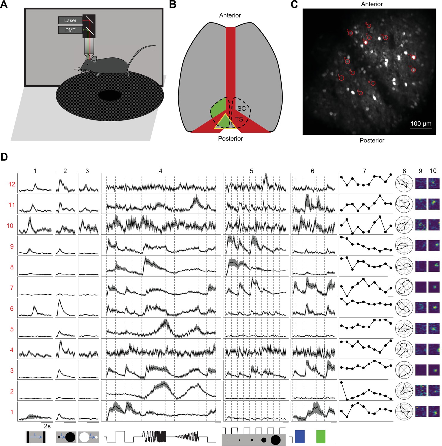
Two-photon imaging reveals diverse visual responses in awake mouse superior colliculus.
(A) Schematic of the experimental setup. Mice were head-fixed and free to run on a circular treadmill. Visual stimuli were presented on a screen. Neuronal calcium activity was imaged using two-photon microscopy. PMT, photomultiplier tube. (B) Schematic of mouse brain anatomy after insertion of a triangular transparent plug to reveal the posterior-medial part of the superior colliculus underneath the transverse sinus. TS: transverse sinus. (C) A standard deviation projection of calcium responses to visual stimuli in one field of view. (D) Response profiles of 12 neurons (rows) marked in C to visual stimuli in the bottom row. Columns 1–6 are time-varying calcium responses to a moving bar, expanding and contracting disks, a ‘chirp’ stimulus with modulation of amplitude and frequency, spots of varying size, and blue and green flashes. Gray shading indicates the standard error across identical trials. Each row is scaled to the maximal response. Scale bars: 2 s. Subsequent columns show processed results: (7) response amplitude to an expanding black disc on 10 consecutive trials. (8) polar graph of response amplitude to moving bar in 12 directions. (9 and 10) Receptive field profiles mapped with small squares flashing On or Off.
Figure 2 with 3 supplements
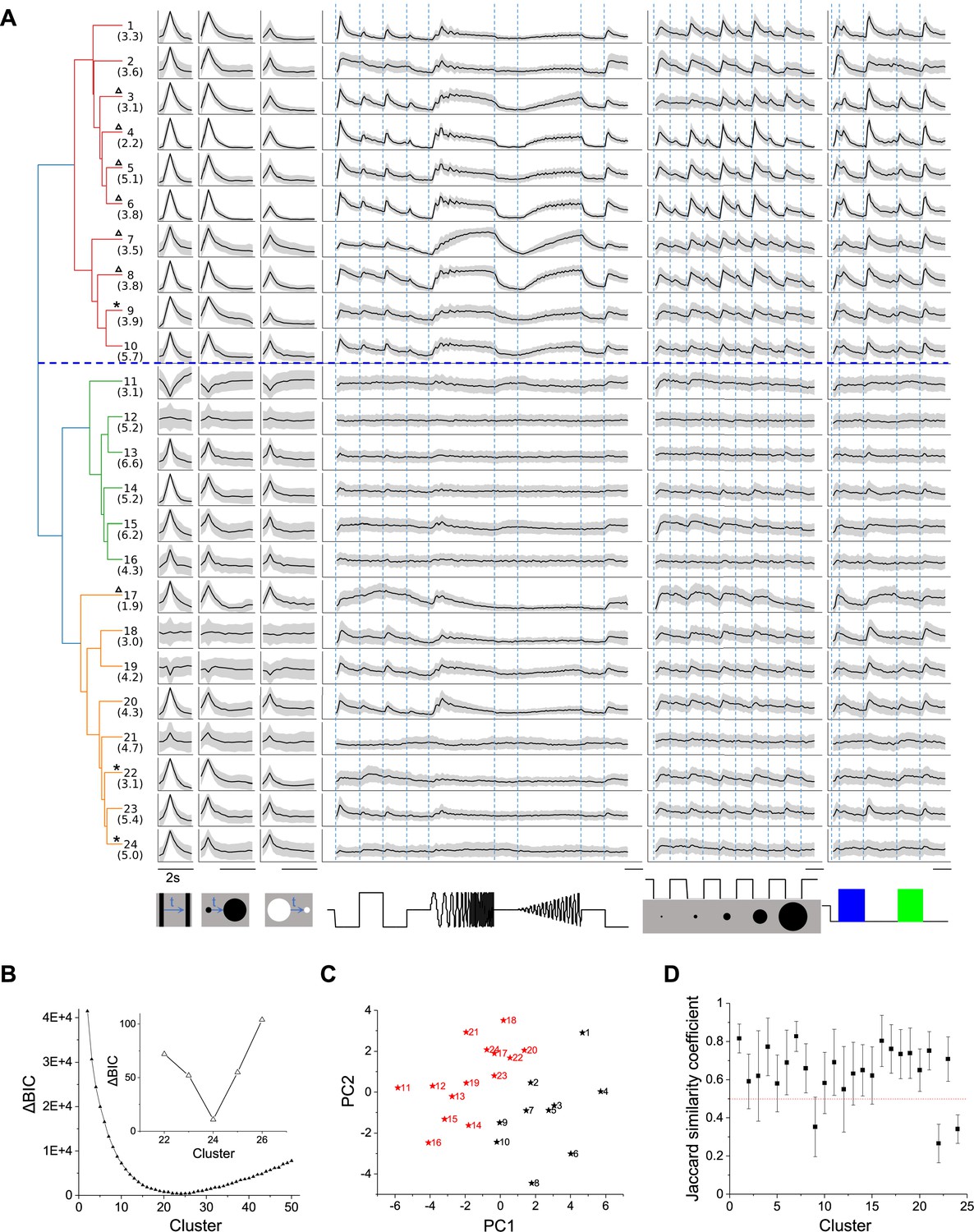
Twenty-four functional cell types in the mouse SC.
(A) Dendrogram of 24 clusters based on their distance in feature space. For each type, this shows the average time course of the neural response to the stimulus panel. Grey: standard deviation. The vertical scale is identical for all types and stimulus conditions. Blue dashed line separates groups 1 and 2. Numbers in parentheses indicate percentage of each type in the dataset. Stars mark the unstable clusters with JSC< 0.5 (see panel D). Triangles mark the clusters where more than half neurons are contributed by one mouse. Scale bars: 2 s. (B) Relative Bayesian information criterion (ΔBIC) for Gaussian mixture models with different numbers of clusters. (C) The center of each cluster in the first two principal axes of feature space. Black and red colors label Groups 1 and 2, respectively. (D) Jaccard similarity coefficient (JSC) between the full dataset and subsets (Mean ± SD).
Figure 2—figure supplement 1
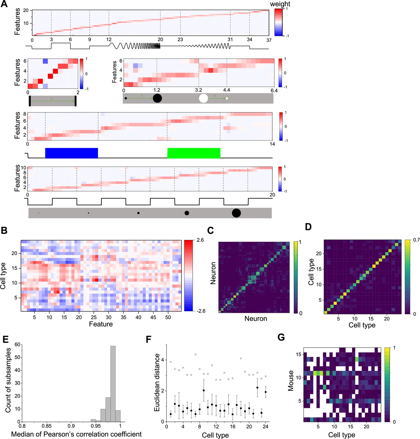
Clustering and validating (related to Figure 2).
(A) Temporal features were extracted from responses to five visual stimuli, including chirp, moving bar, expanding black disc and receding white disc, flashed blue or green squares, and flashed black discs with different sizes. Horizontal axis: time in s. (B) Feature-coefficients for the 24 cell types. Color bar indicates coefficients of features for each cell type. (C) Cell-wise co-association matrix (see Materials and methods). Color bar indicates co-clustering fraction. (D) Between-cluster rate, which is the cluster-wise average of the co-association matrix. (E) Histogram of median correlation coefficients between the original clusters and clusters identified on 100 subsets. (F) Black symbols indicate the Euclidean distance between original clusters and clusters identified on the subsets. Gray symbols indicate the shortest Euclidean distance between the original cluster and other clusters. (G) Contributions of different mice to each of the functional types. White color indicates no contribution.
Figure 2—figure supplement 2
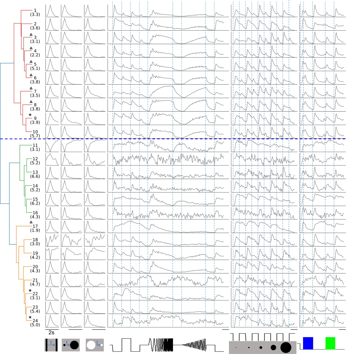
Dendrogram of 24 clusters showing normalized temporal profiles (related to Figure 2).
Figure 2—figure supplement 3
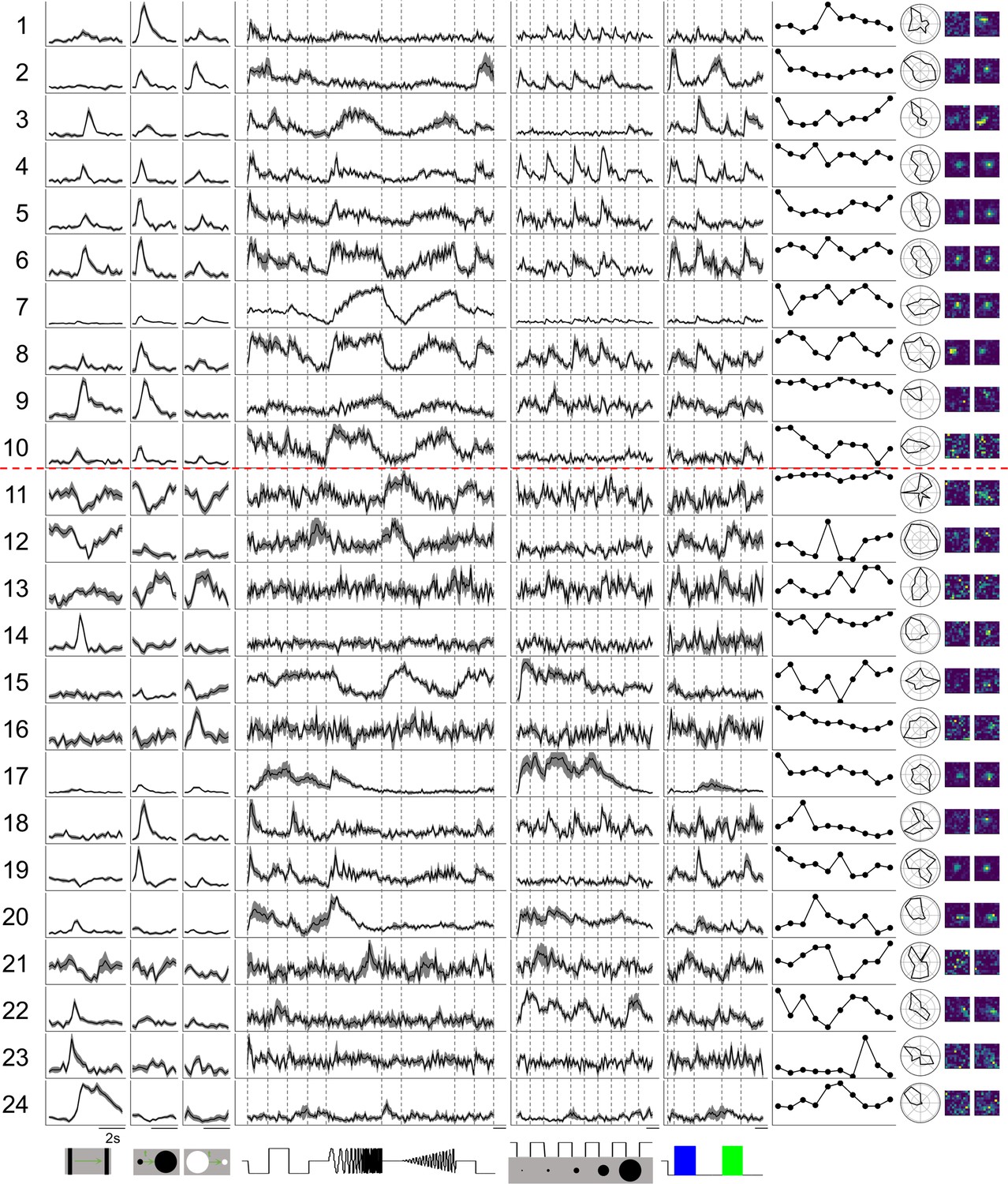
Example responses of single neurons in each type to visual stimuli (related to Figure 2).
Columns 1–6 are time-varying calcium responses to a moving bar, expanding and contracting disks, a "chirp" stimulus with modulation of amplitude and frequency, spots of varying size, and blue and green flashes. Gray shading indicates the standard error across identical trials. Each row is scaled to the maximal response. Scale bars: 2 s. Subsequent columns show processed results: (7) response amplitude to an expanding black disc on 10 consecutive trials. (8) polar graph of response amplitude to moving bar in 12 directions. (9 and 10) Receptive field profiles mapped with small squares flashing On or Off. Red dashed line separates Group 1 and Group 2.
Figure 3 with 1 supplement
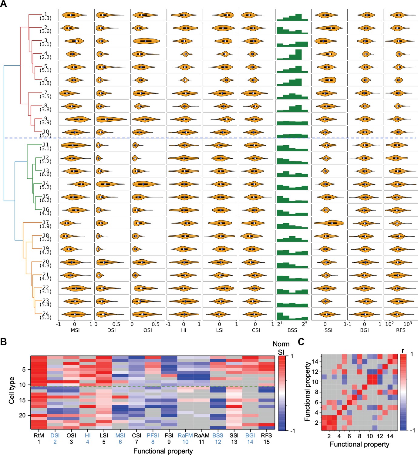
Functional diversity among different types.
(A) Violin plots or histograms of various response indices: motion selectivity index (MSI), direction selectivity index (DSI), orientation selectivity index (OSI), habituation index (HI), looming selectivity index (LSI), contrast selectivity index (CSI), best stimulus size (BSS), surround suppression index (SSI), blue green index (BGI), and receptive field size (RFS). Blue dashed line separates Group 1 and Group 2. (B) Normalized selectivity index (SI, normalized for each column) of functional properties represented by different cell types (See Materials and methods). RtM: response to motion; PFSI: peak-final selectivity index; FSI: frequency selectivity index; RaFM: response after frequency modulation; RaAM: response after amplitude modulation. Gray: values that are not significantly different from 0 (p≥0.05, one-sample t-test). Green dashed line separates Group 1 and Group 2. (C) Pearson’s correlation coefficients of the representation between pairs of functional properties. Gray: non-significant correlations (p≥0.05).
Figure 3—figure supplement 1
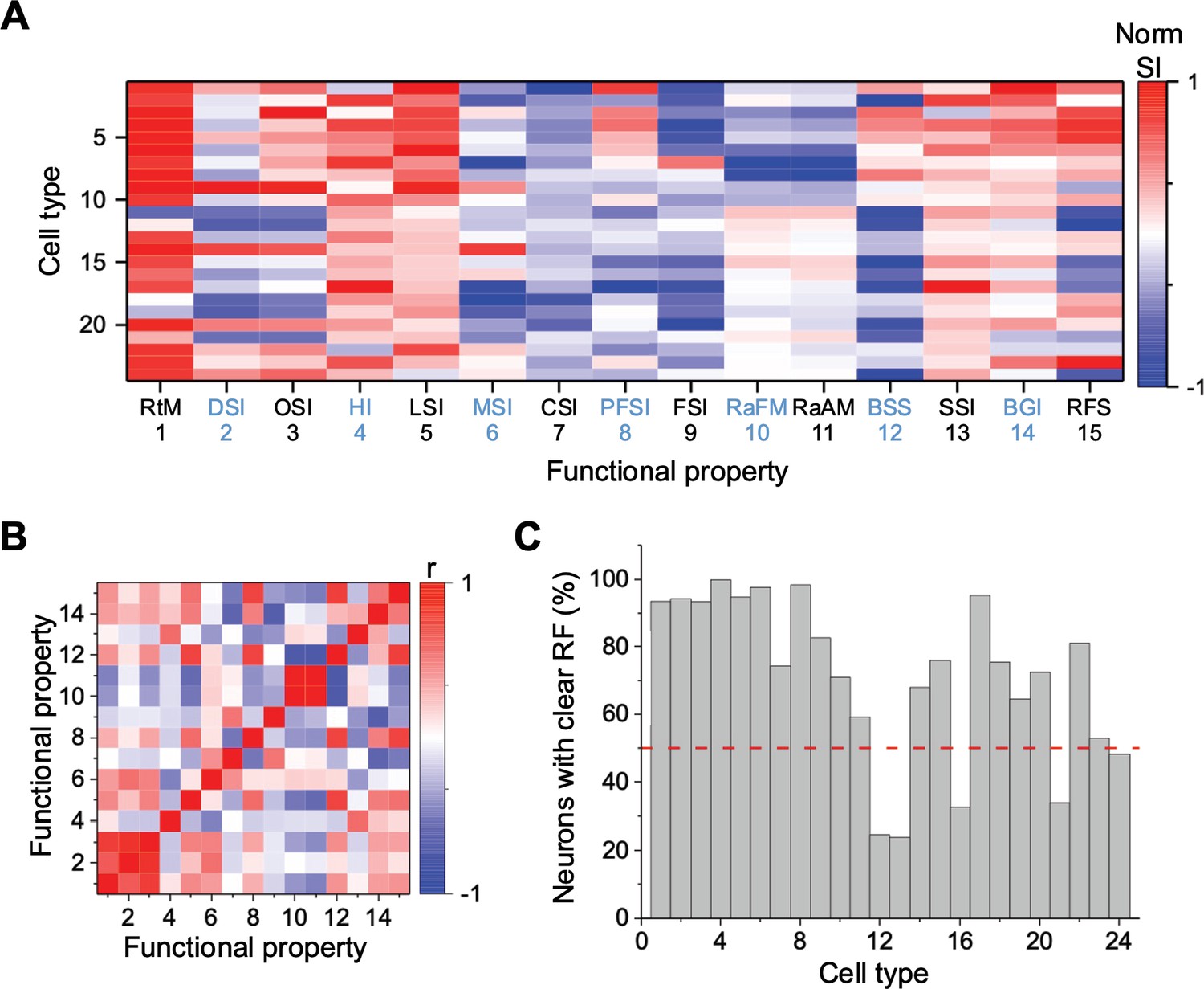
Functional properties of different cell types (related to Figure 3).
(A) Normalized selectivity index (normalized for each column) of functional properties represented by different cell types (see Materials and methods). (B) Pearson’s correlation coefficients of the representation between pairs of functional properties. (C) Percentage of neurons that show clear receptive fields to flash stimuli for each cell type.
Figure 4 with 2 supplements
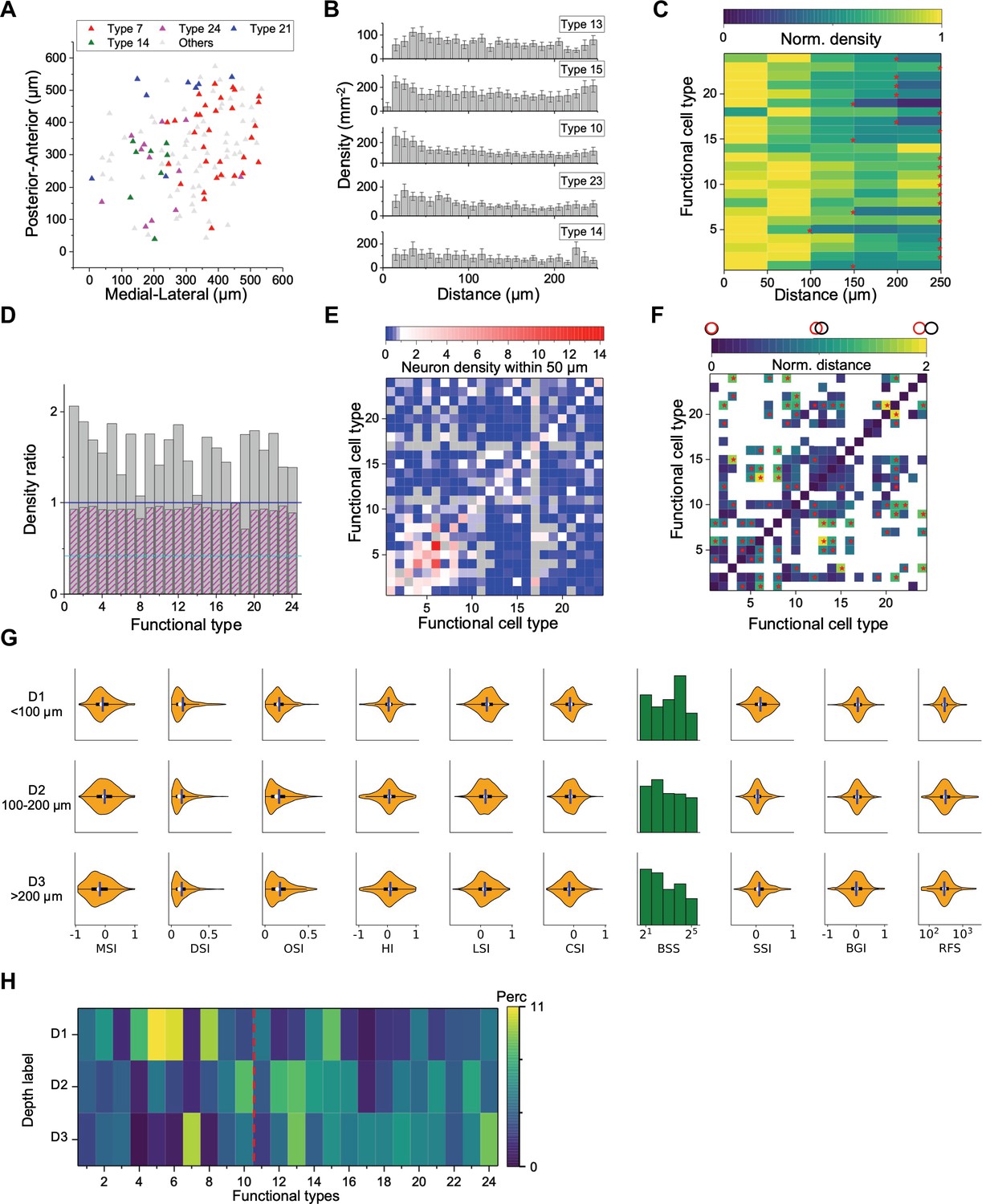
Spatial organization of functional cell types.
(A) Anatomical locations of four types of neurons from one sample recording. (B) Averaged density recovery profile (DRP) of five example types for all imaging planes. Error bars denote SEM. (C) Density of neurons of a given functional type at various distances from a neuron of the same type. Red stars mark the smallest radius within which the neuron density is larger than half of the peak density. (D) Decay of the DRP for each functional type. Gray bars: the ratio between the density at a distance of 0–0.5 RF diameters and the density at 0.5–1 RF diameters. Magenta bars: Same but for cells from all the other types. Cyan line: The value for W3 retinal ganglion cells (Zhang et al., 2012). (E) Density of neurons from different functional types (columns) within 50 μm of a given neuron whose type is indicated by the row. Note the largest density is for cells of the same type except types 8, 11, and 16. Gray: insufficient data to estimate density. (F) Normalized anatomical distance between neurons in any two functional types. Red stars indicate significant separation (p<0.05, bootstrap analysis). White: insufficient data. (G) Functional properties of neurons in three ranges of depth. Display as in Figure 3A. (H) The percentage of functional types in each depth range. Red dashed line separates Group 1 and Group 2.
Figure 4—figure supplement 1
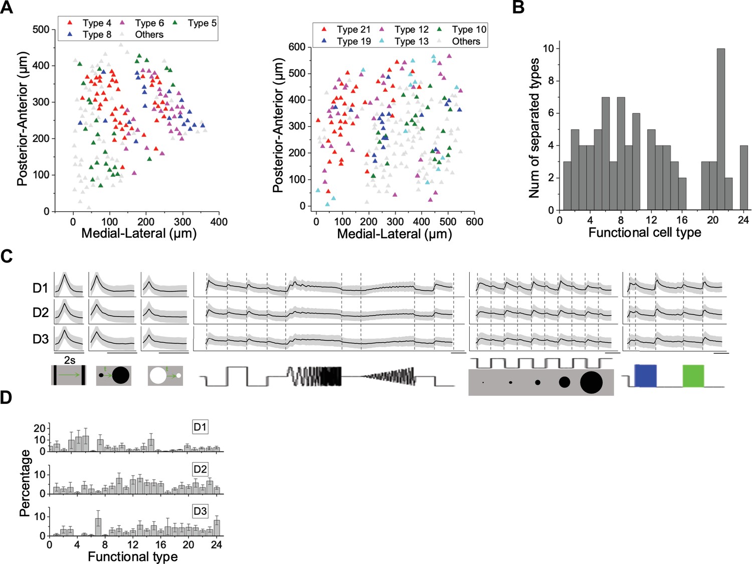
Anatomical organization of functional types (related to Figure 4).
(A) Anatomical locations of different types of neurons in two examples of imaging fields. (B) Number of types that are significantly separated from each reference type (p<0.05, bootstrap analysis). (C) Temporal response across depth. Display as in Figure 2A. (D) The percentage of functional cell types across depth. Error bars denote SEM.
Figure 4—figure supplement 2
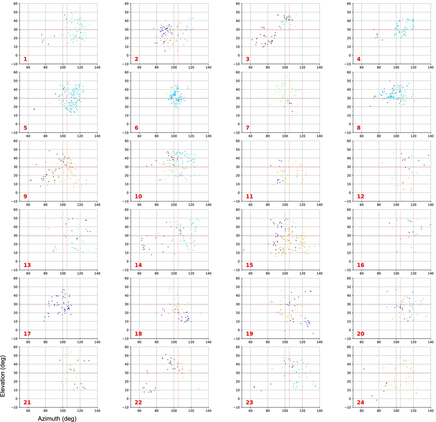
Receptive field center positions for each functional type (related to Figure 4).
Cell types are indicated by the red number at the corner. Color indicates different mice. Axes represent azimuth (horizontal) and elevation (vertical) in degrees. Red cross indicates median azimuth and elevation for all types.
Figure 5
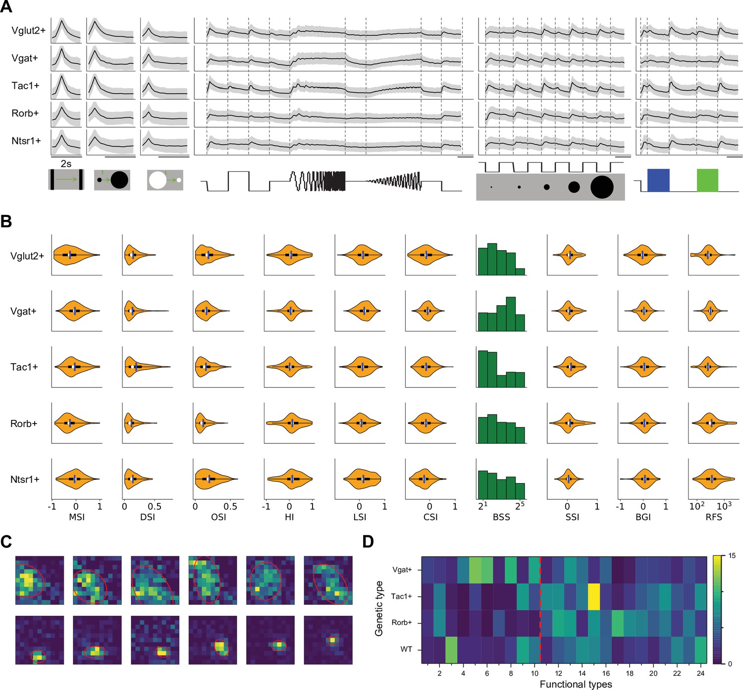
Functional properties in genetically labeled populations.
(A) Average response to the chirp stimulus of five genetically labeled cell types. Display as in Figure 2A. (B) Functional properties of the genetically labeled types. Display as in Figure 3A. (C) Example receptive fields of Ntsr1+ neurons mapped with squares flashing Off and fitted with an ellipse. (D) The percentage of functional types in mice with different genetic backgrounds. Red dashed line separates Group 1 and Group 2.
Figure 6 with 1 supplement

Comparison with functional RGC types.
(A) Weights of different RGC types on each SC type (see Materials and methods). Green dashed line separates Group 1 and Group 2. (B) Plot of mean (triangle) and median (star) OSI versus DSI for 32 functional RGC types. Baden et al., 2016. Color codes functional type. (C) Plot of mean (triangle) and median (star) OSI versus DSI for 24 functional types in the SC. Color codes functional type. (D) PCA of the visual responses of SC and RGC types, plotting the fractional explained variance against the number of components. Inset enlarges the part in the dashed rectangle. The uncertainty in these values was <0.01 (SD) in all cases, as estimated from a bootstrap analysis.
Figure 6—figure supplement 1
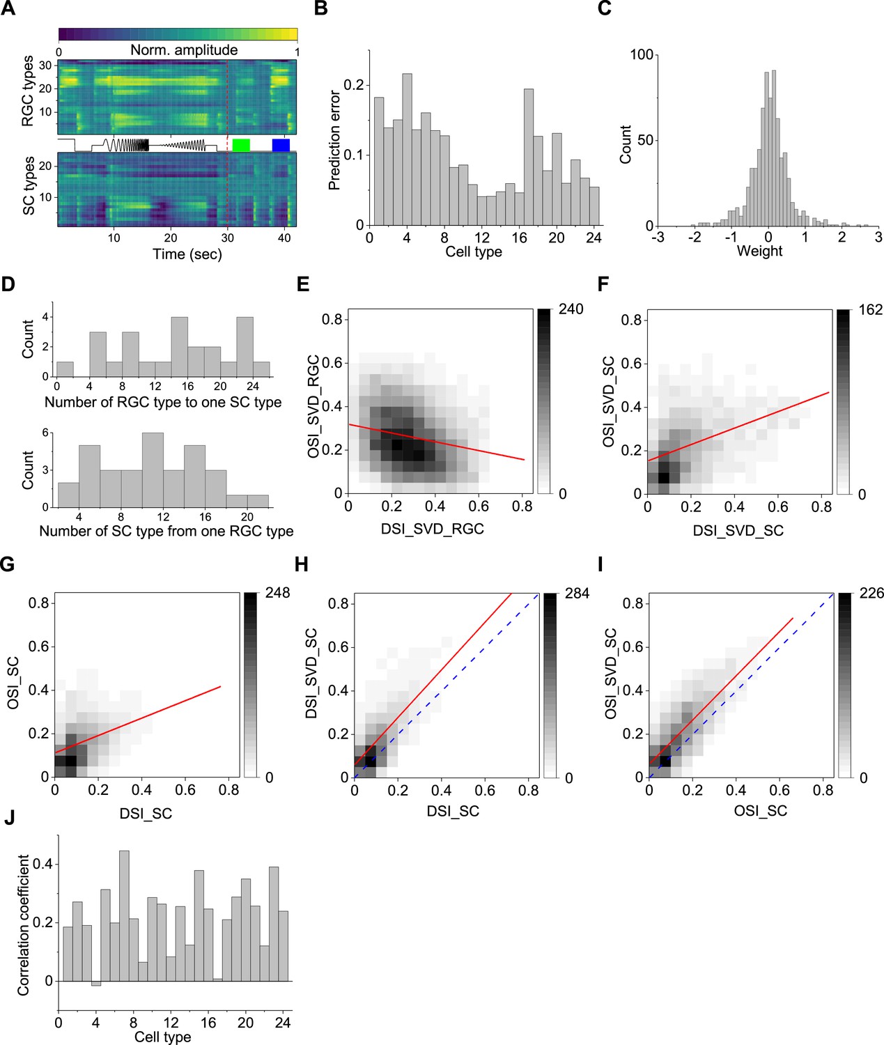
Comparisons between SC neurons and RGCs (related to Figure 6).
(A) Visual responses of RGC types (Baden et al., 2016) and SC types. (B) Prediction error from RGC types to SC types (Equation 28). (C) Histogram of the weights of RGC types to SC types in Figure 6A. (D) If one only considers weights , this histograms the number of RGC types contributing to one SC type, and vice versa the number of SC types with contributions from one RGC type. (E) Plot of OSI vs DSI among RGCs, as reported in Baden et al., 2016. (F) Plot of OSI vs DSI for SC neurons, calculated from the present study by the same SVD algorithm used in Baden et al., 2016. (G) Plot of OSI vs DSI for SC neurons, using the simpler definition from the present study. (H) Plot of DSI for SC neurons, computed by the SVD algorithm (Baden et al., 2016) versus the present definition. Note the close correspondence. (I) As panel (H) for OSI. This analysis shows that the comparison between the retina results in Baden et al., 2016 and SC results in the present study does not suffer from different analysis methods. (J) Correlation coefficients between OSI and DSI for each functional type.
Additional files
Download links
A two-part list of links to download the article, or parts of the article, in various formats.
Downloads (link to download the article as PDF)
Open citations (links to open the citations from this article in various online reference manager services)
Cite this article (links to download the citations from this article in formats compatible with various reference manager tools)
Functional cell types in the mouse superior colliculus
eLife 12:e82367.
https://doi.org/10.7554/eLife.82367


