Sex, strain, and lateral differences in brain cytoarchitecture across a large mouse population
- Department of Computer Science, Open University of Israel, Israel
- Faculty of Biotechnology and Food Engineering, Technion - Israel Institute of Technology, Israel
Figures
Figure 1 with 2 supplements
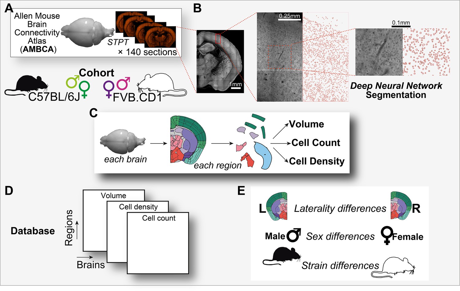
Graphical abstract.
(A) Analysis is based on a cohort of 507 mouse brains from the Allen Mouse Brain Connectivity Atlas (AMBCA), males and females, of C57BL/6J and FVB.CD1 strains. Each brain was imaged in serial two-photon tomography (STPT) and comprises ~140 coronal sections spaced 100 μm apart along the anterior–posterior axis. (B) Example of nucleus segmentation in the isocortex. Each section was divided into tiles of 312 × 312 pixels (109 × 109 μm) (zoom-ins, right). A deep neural network cell segmentation model (see ‘Methods’) was applied to detect the contours of nuclei for downstream analysis across tiles, sections, and whole brains, as shown. (C) For each brain and region that passed QC (see ‘Methods’), volume, cell density, and cell count were computed, resulting in a comprehensive database (D) available through our GUI. (E) The measured variables displayed region-specific laterality differences, sex and strain differences across the population.
Figure 1—figure supplement 1
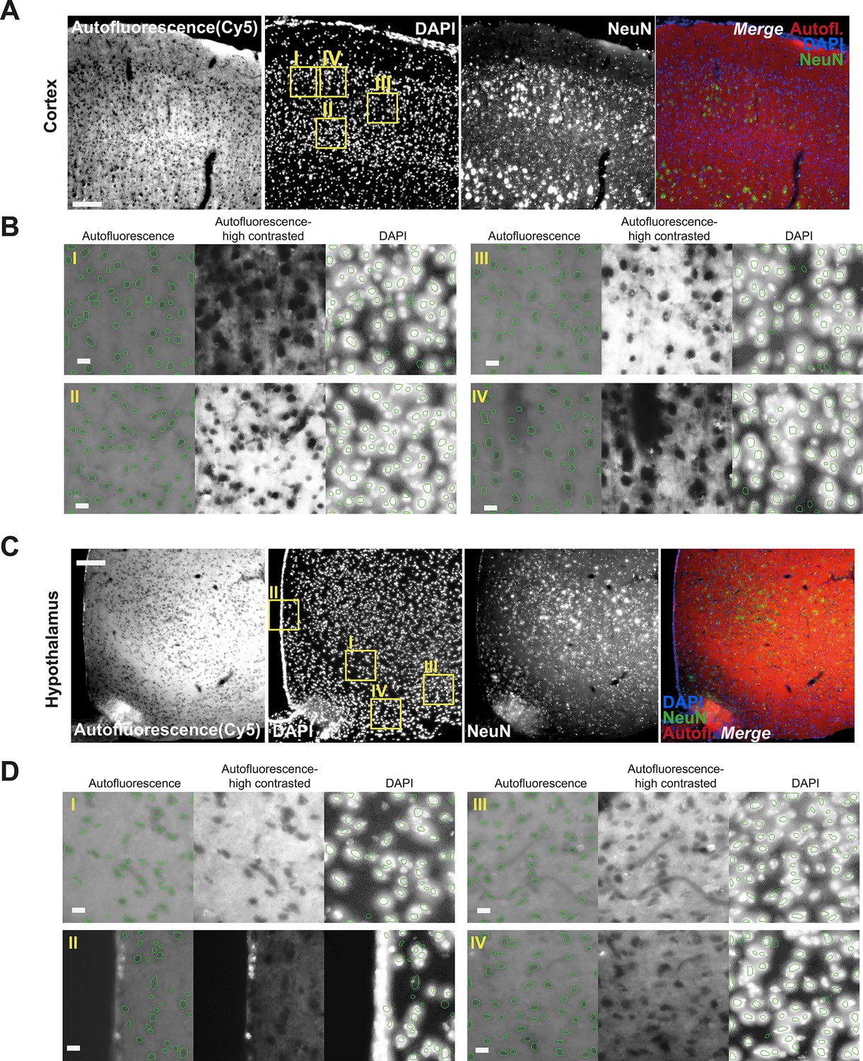
Autofluorescence signal corresponds to nucleus validation.
(A) Mouse brain was perfused with 4% paraformaldehyde (PFA) followed by sectioning, anti-NeuN immunohistochemistry and DAPI counterstaining. Representative image from cortex (A) or hypothalamus (C) showing autofluorescence (Cy5-far red channel), DAPI, NeuN, and the merge of the three channels. (B, D) We applied the same segmentation DNN used for the Allen Mouse Connectivity dataset. Each tile in (B) and (D) shows detected objects on top of the original images (left), autofluorescence high contrast (middle), and DAPI overlayed with the same objects (right). Scale bars, (A and C) 50 μm; (B and D), 10 μm.
Figure 1—figure supplement 2
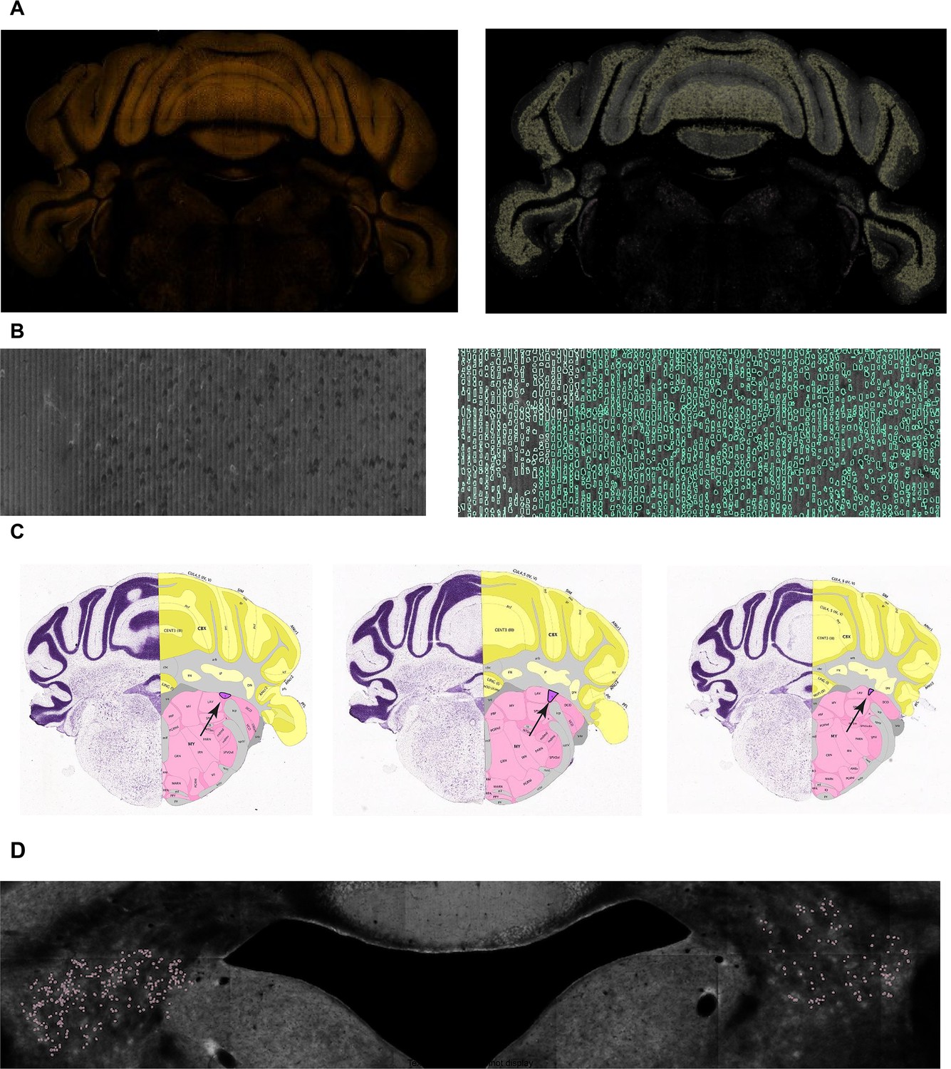
Discarding whole brains or regions of lower technical quality.
(A) A dark image (left; Experiment #112672268 section #110) causing a brain to be discarded. Although the upper part of the image is well segmented (right), the lower part, corresponding to medulla, contains no information. (B) An optical or physical artifact (left; Experiment #268399145 section #77) displaying distinct columns (left). This artifact resulted in the model inaccurately detecting a large number of cells (right). In such cases, whole brains were discarded. (C) Three consecutive slides displaying the Nucleus y (y) region in purple. Such regions of small volume were discarded. (D) An example region for which the difference in cell count between right and left hemispheres was large. In case the average difference was consistently large across brains, the region was discarded.
Figure 2 with 3 supplements
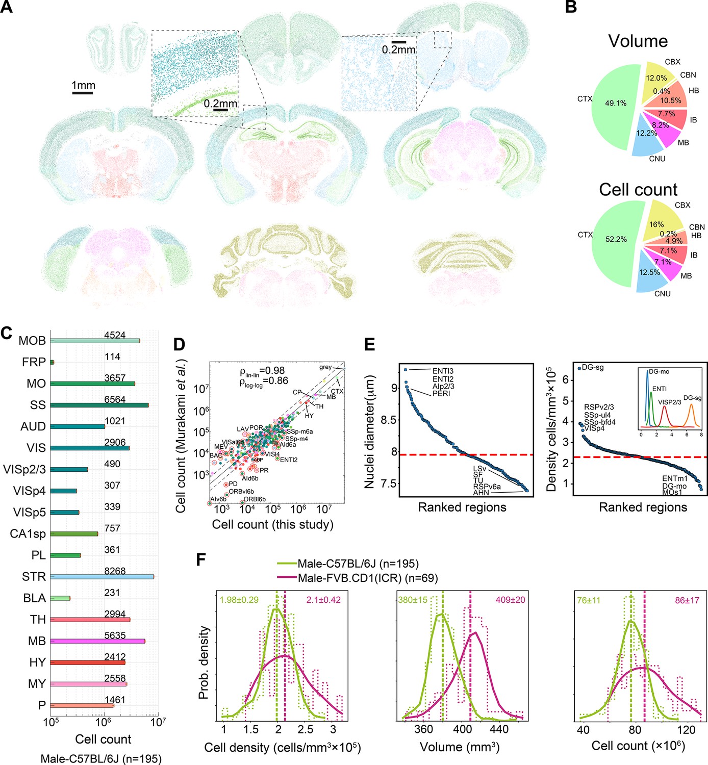
Survey of neuroanatomic properties of the mouse brain.
(A) Segmentation of several sections of one particular brain; segmented nuclei are colored using the Allen Mouse Brain Atlas (AMBA) region convention. (B) Pie charts of the median volumes and cell counts across all 507 brains in the main brain regions, colored using AMBA nomenclature. (CTX: cerebral cortex; CNU: cerebral nuclei; MB: midbrain; IB: interbrain; HB: hindbrain; CBN: cerebellar nuclei; CBX: cerebellar cortex). (C) Median cell counts for selected brain regions in C57BL/6J males (number near bars in thousands; SEM is displayed per region yet values are very small). (D) Comparison of region cell counts between this study and Murakami et al., over C57BL/6J males; dots above/below the dashed lines represent regions with greater than twofold difference. The correlation coefficient in both linear and log scales is displayed. The intraclass correlation coefficient (ICC) values were 0.98–0.99 for six ICC forms. (E) Ranking of 532 regions by nucleus diameter (left) and density (right). Each dot corresponds to the median value of one region over 507 brains. Red dashed line, median across regions. Inset shows distributions of density over 507 brains for selected regions. (F) Distribution of cell density (left), brain volume (middle), and cell count (right), comparing C57BL/6J males and FVB.CD1 males across basic cell groups and regions (‘gray’). Step-like dashed lines represent histograms while full lines correspond to kernel estimations of the probability density function. Dispersion values correspond to standard deviations. Source data for panels (D, E) is provided in Figure 2—source data 1.
-
Figure 2—source data 1
Comparison of cell count per region (male C57BL/6J) with Murakami et al., 2018; median cell diameter and cell density per region over all 507 brains in this study.
- https://cdn.elifesciences.org/articles/82376/elife-82376-fig2-data1-v3.xlsx
Figure 2—figure supplement 1
Technical aspects of 3D cell counting.
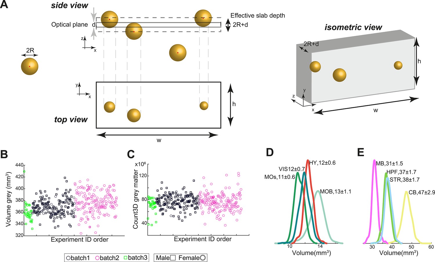
(A) Cell projection onto the section and the relevant volume. Side view: cells in 3D vs. the section plane. Top view: cell projections onto the plane of the section. Cell whose center is more than away from the plane are not counted. Isometric view: the resulting slab for the purpose of density calculation. The slab volume is , hence the density is . (B) Brain gray matter volume as a function of the order by which the experiments were performed by AMBCA. Batches (as indicated by the experiment ID) are designated by different colors. Squares and circles correspond to males and females, respectively. The first batch displays a slightly smaller volume, while the second and batches are almost identical. (C) Same as (B) for total cell count. No batch effect is evident. (D, E) Volume distributions of C57BL/6J regions showing slightly higher variance of main olfactory bulb (MOB) and cerebellum (CB) compared to other regions of the same size.
Figure 2—figure supplement 2

Comparison with quantification based on nuclear staining.
In all panels, the nuclei quantification was made on nine female C57BL/6J brains which were stained by Hoechst and imaged by serial two-photon tomography (STPT) (see ‘Methods’). These brains were compared with 140 female C57BL/6J brains from AMBCA imaged by STPT. Above each panel correlation coefficient (r) is shown together with an intraclass correlation coefficient (ICC) value. (A) Scatter plot of the median per-region volume based on the Allen Mouse Brain Connectivity Project (AMBCA) autofluorescence (x-axis) vs. Hoechst (y-axis), dots are colored according to the Allen Mouse Brain Atlas (AMBA) color code and example region names are noted. The scale is logarithmic, diagonal line represents y = x and dashed lines correspond to twofold difference. (B) Same as (A) for regions’ cell count. (C) Comparison of calculated per-region cell density between Hoechst and AMBCA autofluorescence. Blob size corresponds to region volume. The scale is linear. (C1) cortical regions layer 2/3, 4, 5, and 6a, (C2) cortical regions layer 1 and 6b, (C3) brain stem regions, (C4) cerebellar regions. (D) Per-region ratio (log2 scale) between quantifications, (D1) for cortical layers; (D2) for brain stem and cerebellum.
Figure 2—figure supplement 3
Density and nucleus diameter along cortical regions.
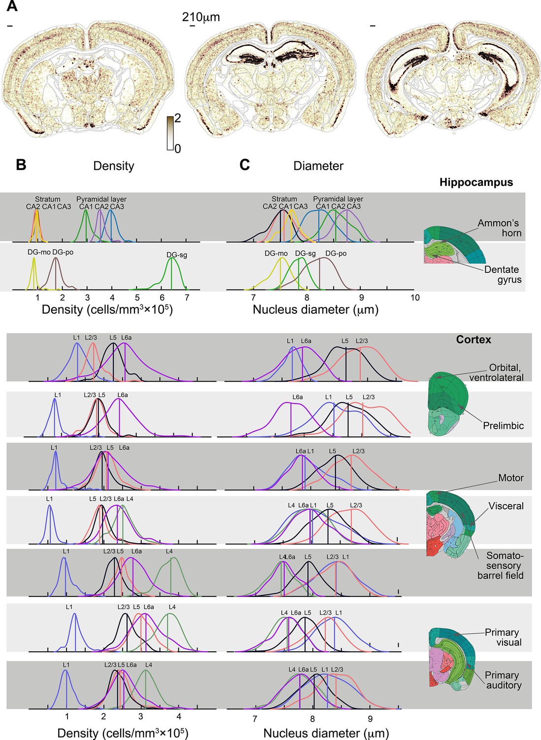
(A) Local density is shown as a heatmap over the anatomy of three coronal sections of one brain. White, low; dark brown, high local density (arbitrary units); scale bars on upper left corners equal 210 μm. (B, C) Distribution of cell density (B) and nucleus diameter (C) in the hippocampus and selected cortical regions, in 195 C56BL/6J male mice. The two upper rows show Ammon’s horn and the dentate gyrus of the hippocampal formation, and the rows below show examples of cortical regions, each resolved to its cortical layers. On the right, approximate locations of each region are indicated in coronal sections of the Allen Mouse Brain Atlas (AMBA).
Figure 3 with 1 supplement

Region-wise laterality of cell densities in C57BL/6J.
(A) Laterality differences in density (all C57BL/6J brains n = 369) shown for all regions whose volume >0.05 mm3 (excluding layers 1 and 6b) resulting in 559 regions. Regions are sorted by their bias to the left. Red and blue dots show layer 2/3 and layer 5/6a, respectively. Upper inset shows the distribution of layer 2/3 regions and layer 5/6a in red and blue lines, respectively. (B) Scatter plot of the density of the left vs. right hemisphere for parasubiculum (PAR). Each dot corresponds to one brain. Vertical and horizontal cyan lines correspond to the left and right median values, respectively. The dashed dotted line is equi-density value and the dashed line corresponds to a 10% offset by the median of the left density. The inset shows an analogous scatter plot for volume, with no observed lateral bias. (C) Percentage of brains with tendency for left or right hemisphere density across cortical areas (blue, left > right; orange, right > left). (D) Scatter plots of the density of the left vs. right hemisphere for visceral area layers 2/3, 4, 5, and 6A.
Figure 3—figure supplement 1

Volcano plots showing region-wise comparison of left vs. right hemispheres in C57BL/6J and FVB.CD1.
(A, B) Density comparisons for C57BL/6J and FVB.CD1, respectively. (C, D) The same for volume.
Figure 4 with 1 supplement
Sexual dimorphism in C57BL/6J.
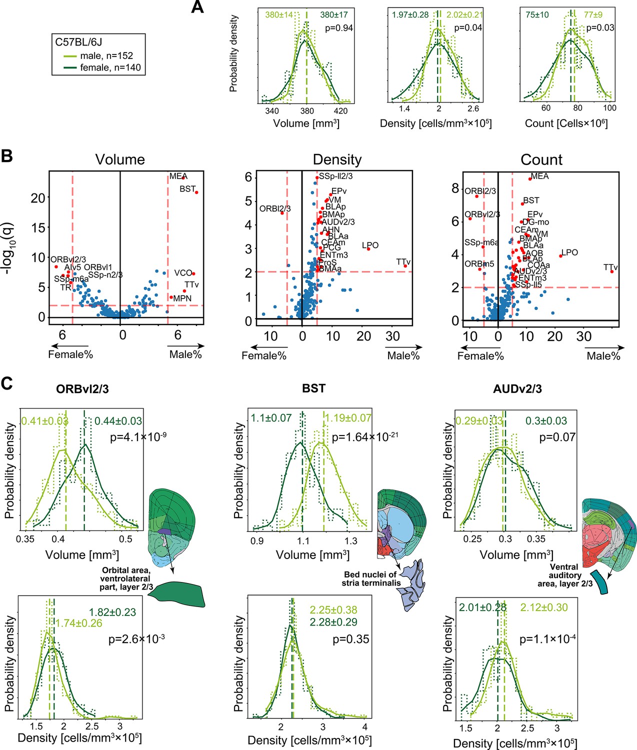
(A) Distribution of volume (left), density (middle), and cell count (right) for the whole brain gray matter (‘gray’) in female (dark green), and male (light green). p-Values correspond to a rank-sum test. Step-like dashed lines represent histograms while full lines correspond to kernel estimations of the probability density function. Dispersion values correspond to standard deviations. (B) Volcano plots showing per-region statistical testing for male versus female difference in volume (left), density (middle), and cell count (right), each dot representing one region. Horizontal axis, median differences (%); vertical axis, q-values (FDR-corrected rank-sum p-values by BH procedure in -log10 scale). Red dots highlight regions with an effect size larger than 5% and q < 0.01. Source data for this panel is provided in Figure 4—source data 1. (C) Examples of regions that display sexually dimorphic volume and/or density. Distributions of volumes appear in the upper row, distributions of densities in the lower row.
-
Figure 4—source data 1
Median values per region for cell count, volume and cell density for male and female C57BL/6J or FVB.CD1.
- https://cdn.elifesciences.org/articles/82376/elife-82376-fig4-data1-v3.xlsx
Figure 4—figure supplement 1
Validation and additional aspects of sexual dimorphism.
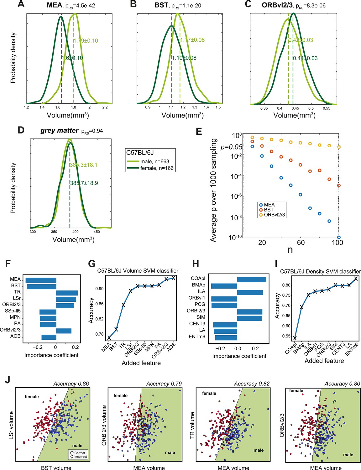
(A–D) Independent validation of region-specific sexual dimorphism in C57BL/6J. Using data from an independent cohort of 663 males vs. 166 females, we display the volume distributions of regions found to display dimorphism in our basic cohort – medial amygdala (MEA) (A), bed nuclei of the stria terminalis (BST) (B), and ORBvl2/3 (C). Also shown is the similarity between whole-brain volumes (D). p-values are based on a rank-sum test. (E) The average p-value for sexual dimorphism in MEA (blue), BST (red), and ORBvl2/3 (blue) as a function of sample size. Specifically, n males and n females from our cohort were randomly selected and the rank-sum p-value was calculated. Shown is the average p-value over 1000 such random selections. (F) Top 10 regions when constructing a linear support vector machine (SVM) volume-based classifier. (G) Accuracy of volume-based classifiers when using the top 10 regions, adding one region at the time. (H, I) Same as (E, F) but for density-based classifiers. (J) Four examples of two-dimensional SVM based on volume information, as indicated on x and y axes; with accuracies indicated above. The separating line splits the plane into female/male domains. Red/blue markers represent individual males and females, respectively. Circles and diamonds represent correct and incorrect classifications, respectively.
Figure 5
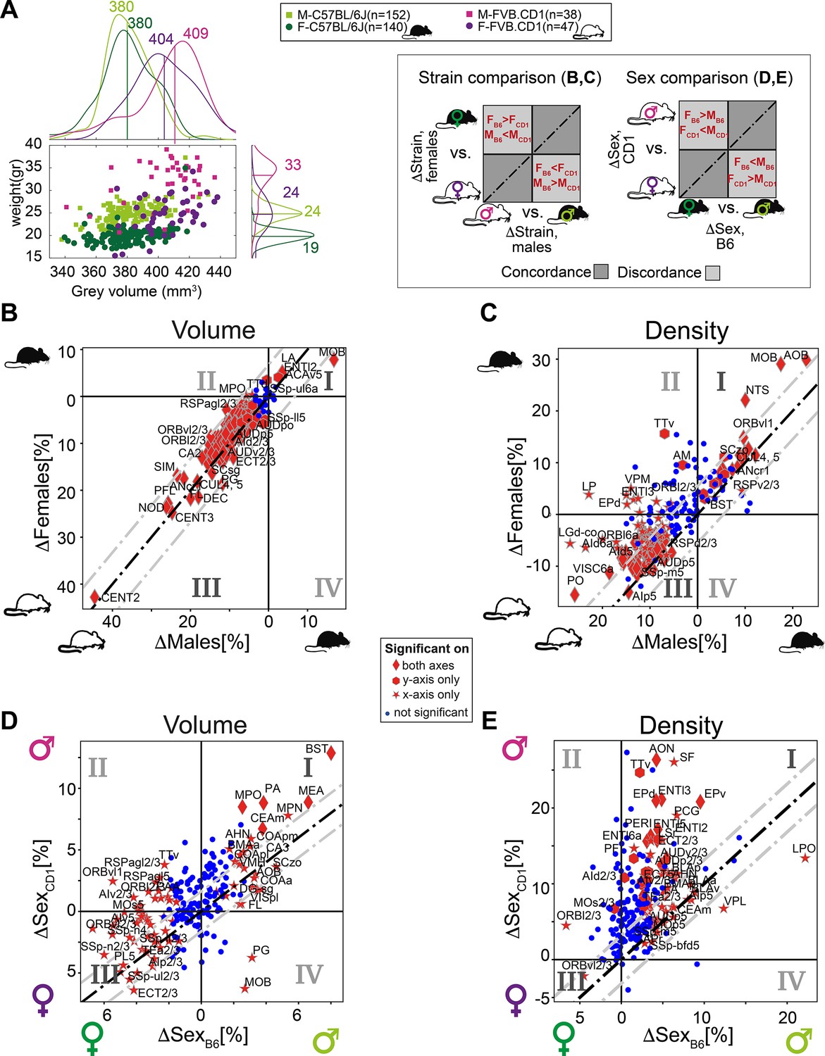
Sexual and cross-strain dimorphism in C57BL/6J (B6) and FVB.CD1 (CD1).
(A) Scatter plot showing body weight vs. gray volume for 507 brains. Side panels show the group distributions of gray matter volume (upper) and weight (right). Lines are the medians whose values are indicated. (B, C) Strain comparison of per-region volume (B) and density (C). Differences between the median values of the strains, per region, are shown for males (horizontal axis) and females (vertical axis). Points in quadrants I and III suggest concordance between males and females across strains, as illustrated in the schematic on the left. Red markers designate statistical significance (q-value < 0.05) in either axes or in both. (D, E) Sex comparison of per-region volume (D) and density (E). Points in quadrants I and III suggest concordance between C57BL/6J and FVB.CD1 across sex, as illustrated in the schematic on the left. Source data for panels (A–E) is provided in Figure 5—source data 1.
-
Figure 5—source data 1
Volume and body weight per mouse; strain differences in volume or cell density for male and female; sex differences in region volume or cell density for C57BL6 and FVB.CD1.
- https://cdn.elifesciences.org/articles/82376/elife-82376-fig5-data1-v3.xlsx
Figure 6 with 1 supplement
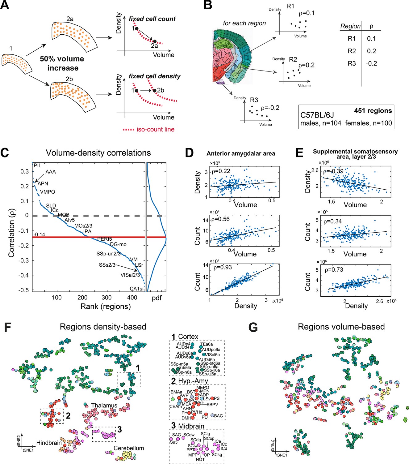
Correlations between volume, cell count, and density.
(A) Schematic illustration of two types of relations between regional cell density and volume, associating region expansion with a fixed number of cells (upper) or with a fixed density (lower). Each regional expansion can be represented by a shift in the volume–density plane (right column). (B) A scheme showing how for each region the correlation between density and volume was measured over the whole dataset. (C) Brain regions ranked by the correlation between volume and density based on C57BL/6J (104 males, 100 females). Correlations higher than 0.14 or lower than –0.14 correspond to q-values lower than 0.05. Side panel displays the distribution of correlation values, and its median is denoted by the red line. Arrows point to regions mentioned in the following panels. (D) Correlations between volume, density, and count in the anterior amygdalar area (AAA). (E) As (D), for supplemental somatosensory area, layer 2/3 (SSs2/3). (F, G) Visualizing similarity between brain regions across the population, by tSNE embedding on pairwise correlations between region density (F) or region volume (G). Each dot represents a region and is colored according to the Allen Mouse Brain Atlas (AMBA) convention. Dashed rectangles indicate zoom-ins on three frames on each tSNE.
Figure 6—figure supplement 1
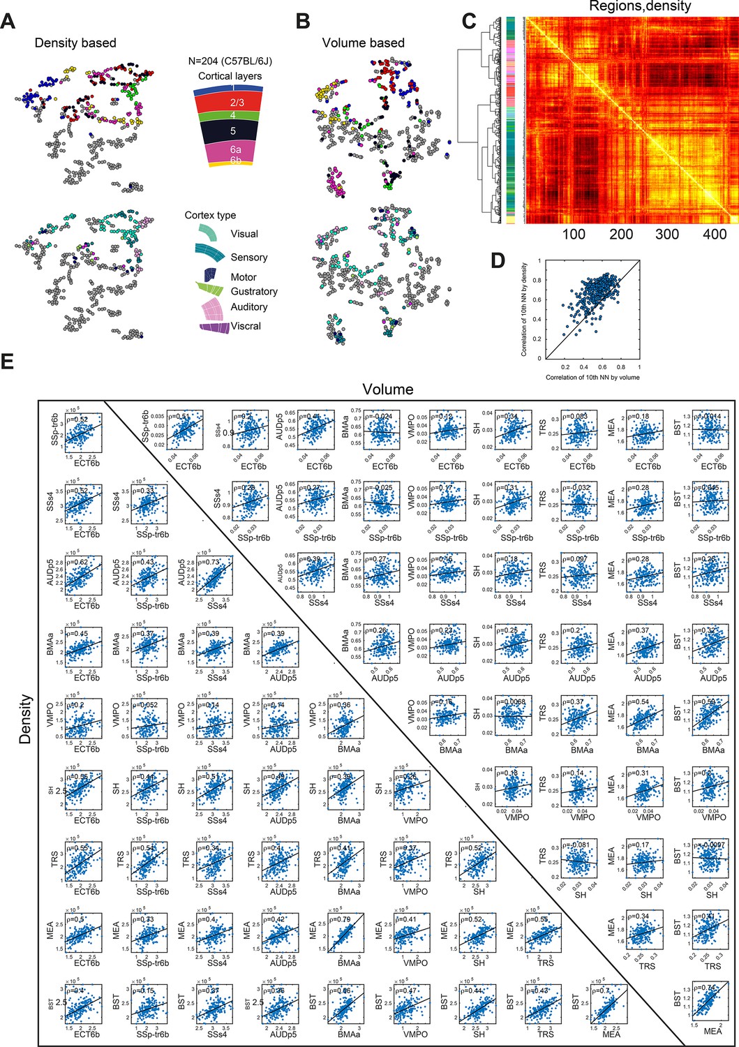
Region to region correlation within the C57BL/6J population.
(A) tSNE as shown in Figure 5F, each dot is a region and tSNE is calculated based on density data of 204 C57BL/6J mice. Upper panel shows different cortical layers (color code on the right) and lower panel show different cortical regions. (B) Same as (A) but for tSNE based on volume data. (C) The heatmap corresponding to the similarity between pairs or regions based on their density across 204 C57BL/6J brains (451 regions). The tSNE plots correspond to a 2D embedding of this heatmap. (D) Region-to-region correlation matrix based on density data, and order of region is based on hierarchical clustering (linkage), which is shown on the left. A bar with the region color code is shown to the left of the heatmap. (E) Scatter plot showing the 10th best correlation of each region when is calculated in the volume data (x-axis) or density data (y-axis). (E) example scatter plots showing the correlation between pairs of regions based on volume (upper triangular) or density (lower triangular). The examples are shown on a representatives set of preselected regions, BST, ECT6b, SSp-tr6b,SSs4, AUDp5, BMAa, VMPO, SH, TRS, and MEA.
Author response image 1

Heatmap of ISH data for five genes across brain regions .
Tables
Table 1
Breakdown of the data by strain and sex.
| Strain | Females | Males | Total |
|---|---|---|---|
| C57BL/6J | 174 | 195 | 369 |
| FVB.CD1(ICR) | 69 | 69 | 138 |
| Total | 243 | 264 | 507 |
Table 2
Model performance over out-of-sample tiles.
| Segmentation (pixel-wise) scores | Detection (cell-wise) scores | |||||
|---|---|---|---|---|---|---|
| Region | # cells in the test set | Jaccard index | F1 | Total errors | Accuracy | False positive rate |
| Isocortex | 192 | 0.982 | 0.991 | 0.002 | 0.962 | 0 |
| MEA | 115 | 0.975 | 0.987 | 0.001 | 0.962 | 0 |
| HY | 163 | 0.953 | 0.974 | 0.003 | 0.938 | 0.005 |
| HIP | 566 | 0.986 | 0.992 | 0.001 | 0.979 | 0.009 |
-
MEA: medial amygdala; HY: hypothalamus; HP: hippocampus.
Additional files
Download links
A two-part list of links to download the article, or parts of the article, in various formats.
Downloads (link to download the article as PDF)
Open citations (links to open the citations from this article in various online reference manager services)
Cite this article (links to download the citations from this article in formats compatible with various reference manager tools)
Sex, strain, and lateral differences in brain cytoarchitecture across a large mouse population
eLife 12:e82376.
https://doi.org/10.7554/eLife.82376


