A pH-dependent cluster of charges in a conserved cryptic pocket on flaviviral envelopes
- Bioinformatics Institute (A*STAR), Singapore
- Department of Chemistry, Manchester Institute of Biotechnology, The University of Manchester, United Kingdom
- Department of Biological Sciences, 16 Science Drive 4, National University of Singapore, Singapore
- Department of Chemistry, The Pennsylvania State University, United States
- School of Biological Sciences, Faculty of Biology, Medicine and Health, Manchester Institute of Biotechnology, The University of Manchester, United Kingdom
Figures
Figure 1 with 1 supplement
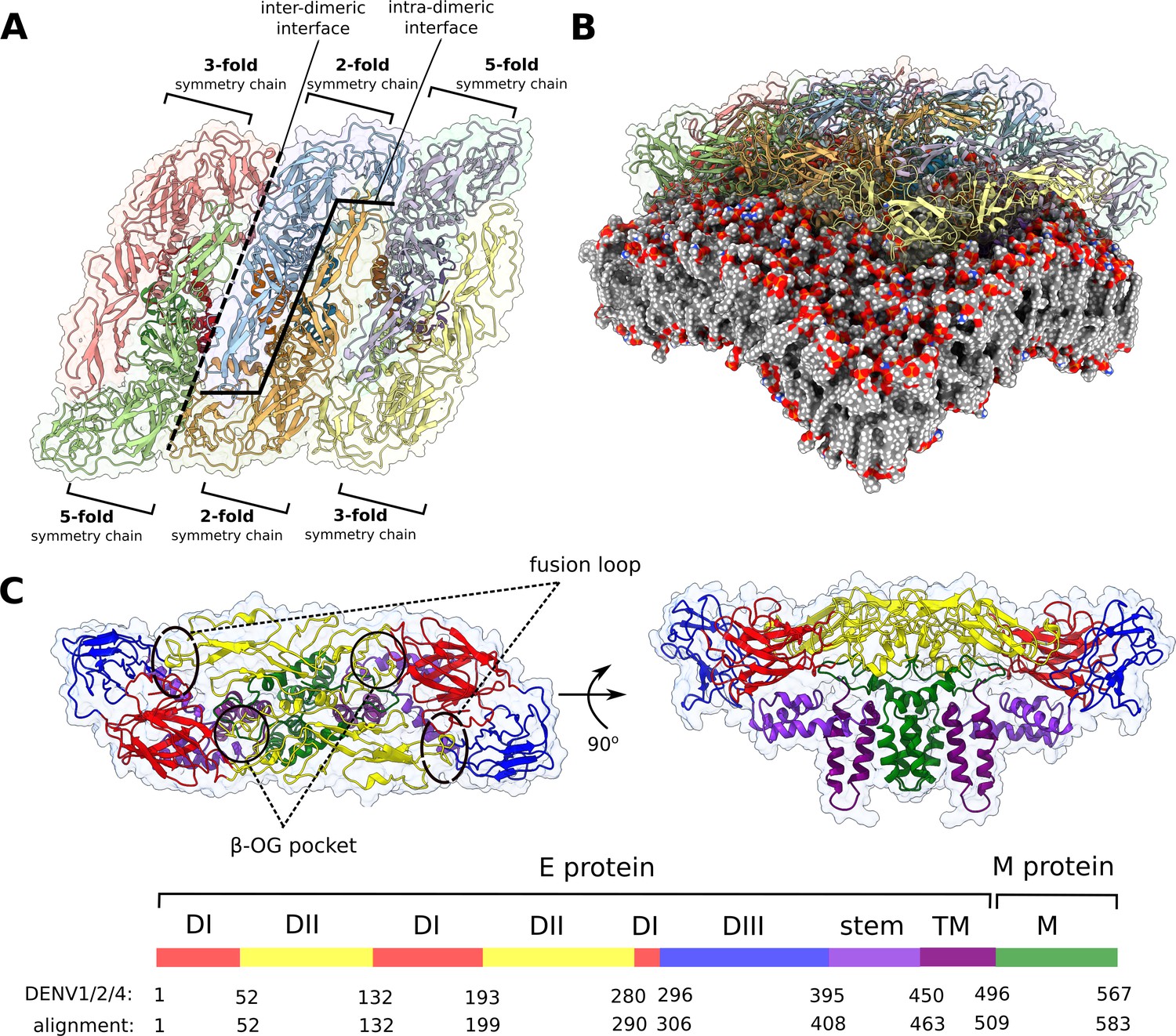
Flaviviral raft structure and domain organisation.
(A) A top-down view on the flaviviral envelope protein raft consisting of three E2M2 heterotetramers organised in a parallel fashion. Chains differ in the context of their immediate environment and are described in terms of the symmetry fold, which is repeated across the entire viral particle. In this model, the majority of interchain contacts is retained for the central dimer (consisting of two 2-fold symmetry chains), while the edge 3-fold symmetry chains are not bordering neighbouring rafts as in the full virion. (B) The curvature of the envelope membrane is imposed by that of the protein rafts. See also Figure 1—figure supplement 1. (C) Top and side views of the E2M2 heterotetramer shown in ribbon representation and coloured by functional domains. Protein surface is shown as a transparent outline. The six flaviviral strains differ in length, and residue numbers on the key correspond to the alignment of all strains and to DENV1, 2, and 4. By convention, individual residues mentioned in the text are always matched with DENV2 numbering.
Figure 1—figure supplement 1
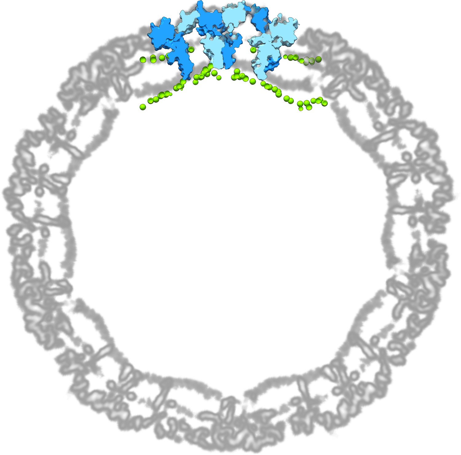
An atomistic model of a DENV2 raft and its curved membrane overlaid with a cryo-EM map of a DENV2 envelope (PDB: 3J27; EMDB: EMD-5520).
The EM map is depicted as a single plane spanning the centre of the viral particle. For clarity, the raft model is visualised as a thin slice overlaid with the cryo-EM map. Raft chains are shown in alternating light and dark blue surfaces, while membrane phosphorus atoms are shown in green spheres.
Figure 2
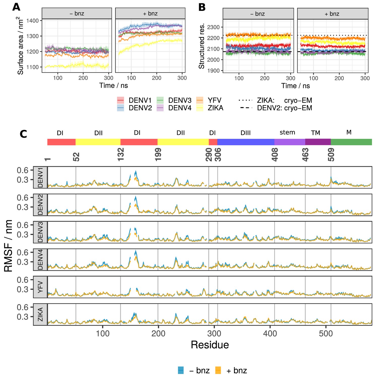
Global raft properties for all six viral serotypes showing the effect of benzene probes added to the solvent.
(A) The total SASA across all viral systems increases with the addition of hydrophobic benzene probes to the solvent. The first 50 ns of each simulation was considered as equilibration and therefore omitted from the analysis. (B) The number of residues participating in secondary structure (defined as constituent elements of ⍺-helices, β-sheets, β-bridges, or turns) remains largely unaffected in benzene systems and closely corresponds to the values describing the experimentally derived cryo-EM structures. (C) The RMSF values describing whole-residue fluctuations are similar across solvent types and viral serotypes. The gaps in lines are due to the sequence alignment which accounts for differences in length or deletions/insertions between different flavivirus envelope proteins, ensuring that the corresponding residues are vertically aligned. All values displayed in panels are averaged across repeats and, in the case of RMSF, across all chains of the system. Standard error is shown as a transparent ribbon around the mean value.
Figure 3 with 1 supplement
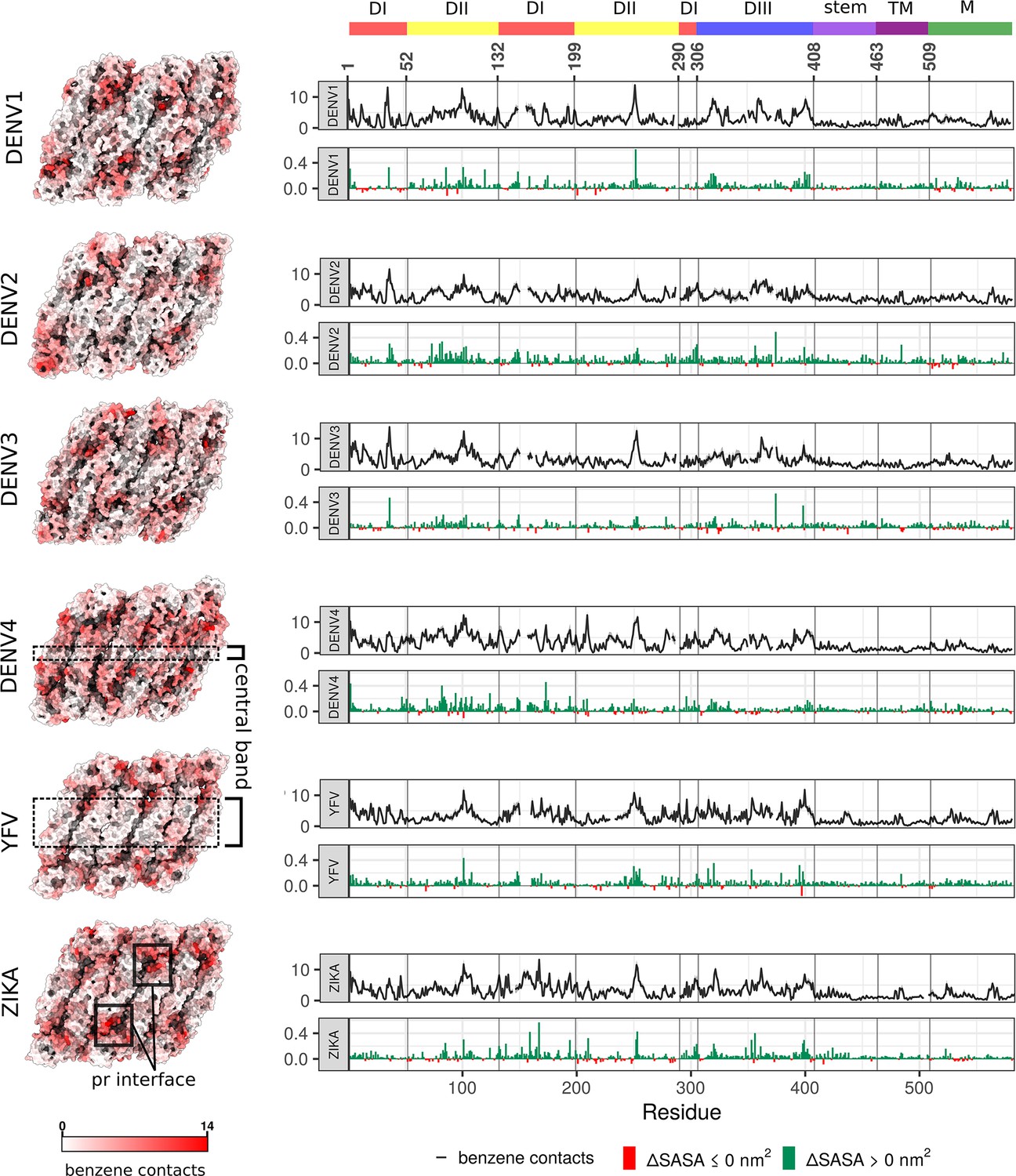
Benzene contacts and changes in SASA shown for all six viral serotypes.
(Left) The average number of benzene contacts per residue is shown on viral raft structures. The values for individual chains are averaged across repeats. For patterns of residue conservation and phylogenetic relationships between strains, see Figure 3—figure supplement 1. (Right) In each upper graph, the mean value of benzene contacts per residue averaged across all chains and repeats is shown in black line, with standard error displayed as a grey ribbon. In each lower graph, the average change in SASA is shown in nm (Bhatt et al., 2013), calculated as (SASA+bnz - SASA-bnz), with an increase shown in green and decrease in red. As with Figure 2, the gaps in lines are due to flavivirus-specific sequence alignment.
Figure 3—figure supplement 1
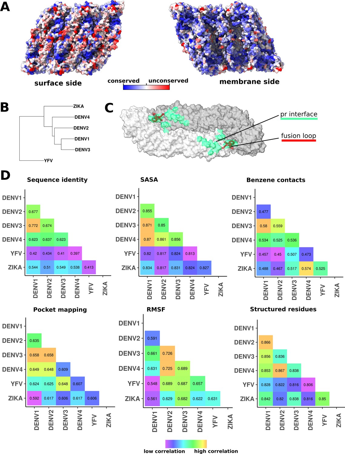
Residue conservation and phylogenetic relationships of flaviviruses correlated with simulation properties.
(A) Raft residue conservation as shown on the raft surface. The surface side is turned towards the exterior of the viral particle, while the membrane side is interacting with the lipid bilayer and is for the most part hidden from the host immune system. (B) Phylogenetic relationship of six flaviviruses presented by an unrooted neighbour joining (NJ) tree. DENV1 and DENV3 are most closely related viral serotypes, while YFV is comparatively distant in evolutionary terms to the DENV group. (C) The E protein dimer showing the pr interface (green surface) and the fusion loop (red ribbon; residues 98–111). The dimer is shown in a surface representation with individual chains coloured in shades of grey. (D) Correlation analyses of properties associated with the selected viral serotypes. Sequence identity matrix shows percentage identity of E and M protein sequences in a pairwise fashion. This matrix reflects evolutionary relationships between viruses shown in panel B. Other matrices display pairwise correlations of viral properties obtained from MD simulations. The values of SASA, RMSF, and number of structured residues were derived from water-only simulations, while benzene contacts and pocket densities were taken from benzene simulations. All correlations were calculated using the Spearman’s rank correlation coefficient method.
Figure 4 with 1 supplement
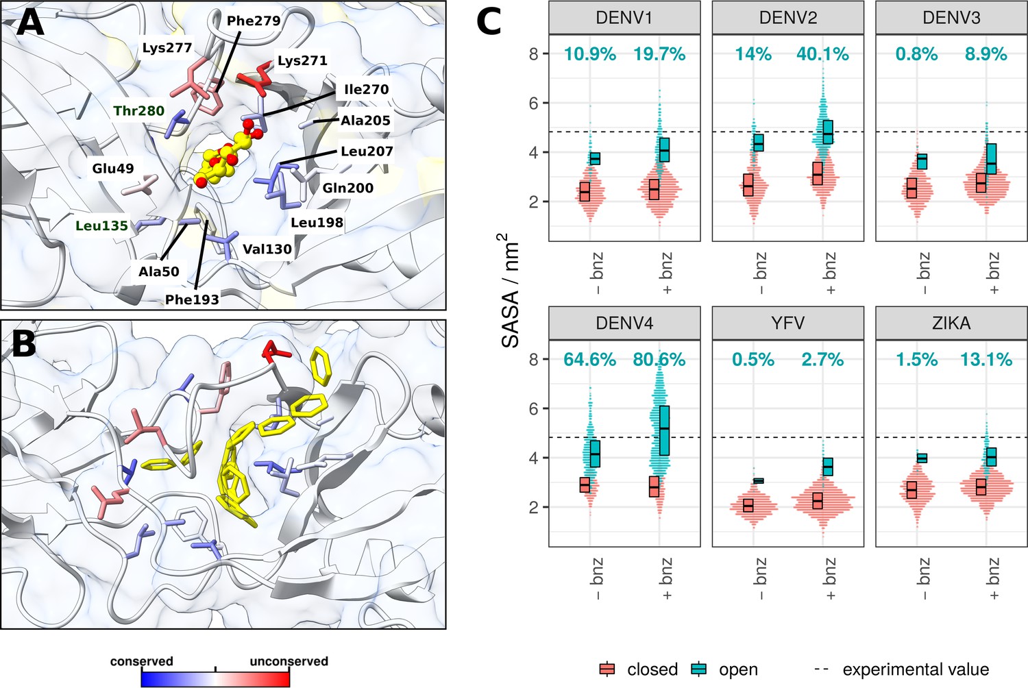
β-OG pocket in the presence of the β-OG ligand or benzene, and its SASA across viral serotypes.
(A) The β-OG detergent molecule co-crystallised inside the cryptic pocket of the DENV2 sE protein (PDB code: 1OKE) (Modis et al., 2003) . The protein is shown as a combination of white ribbon and transparent surface representations. The β-OG molecule is shown in yellow sticks, with oxygen atoms highlighted in red. The residues surrounding the ligand are accentuated in stick representation and coloured based on their conservation scores calculated in Consurf (Ashkenazy et al., 2016). Residue labels correspond to DENV2. (B) A representative simulation snapshot of benzene molecules occupying the β-OG pocket in the DENV2 system. Benzenes are shown in yellow stick representation. Other elements of the system are visualised in the same way as in panel A. (C) Cumulative SASA for all residues lining the pocket (labelled in panel A) across six flaviviral serotypes. The data was visualised as a swarm plot, where a SASA measurement for each sampled frame was represented as a horizontally stacked non-overlapping point. The spread of points therefore describes the distribution of SASA measurements for systems in absence (-bnz) or presence of benzene (+bnz). Pocket SASA values are shown separately depending on the solvent composition. Open and closed conformations of the pockets were differentiated by applying a k-means clustering algorithm (details in the Methods section). The percentage of the β-OG pocket observed in an open conformation is specified for each simulation system. The indicated experimental SASA value of the pocket is that measured for the crystal structure (panel A) averaged across the two chains. See also Figure 4—figure supplement 1.
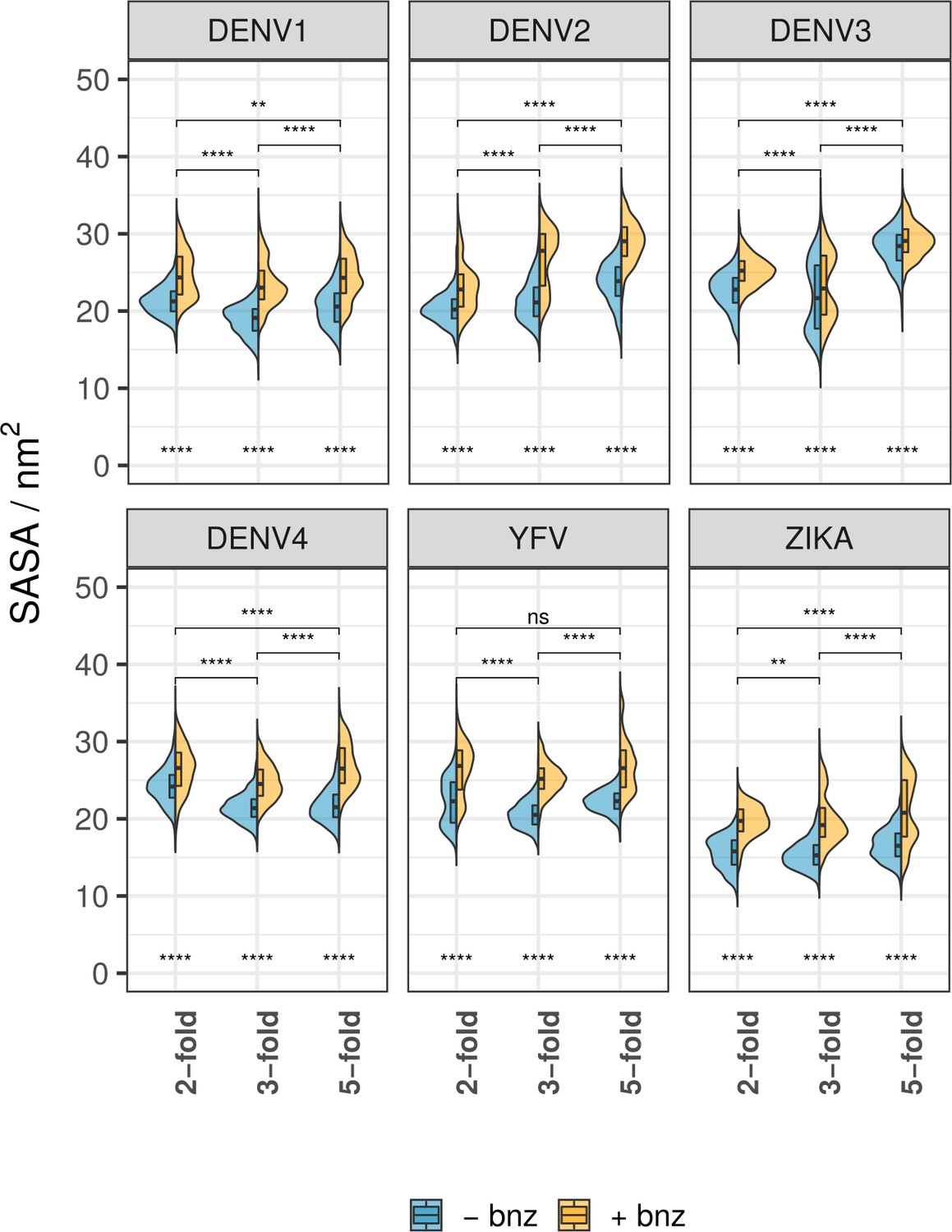
Figure 4—figure supplement 1
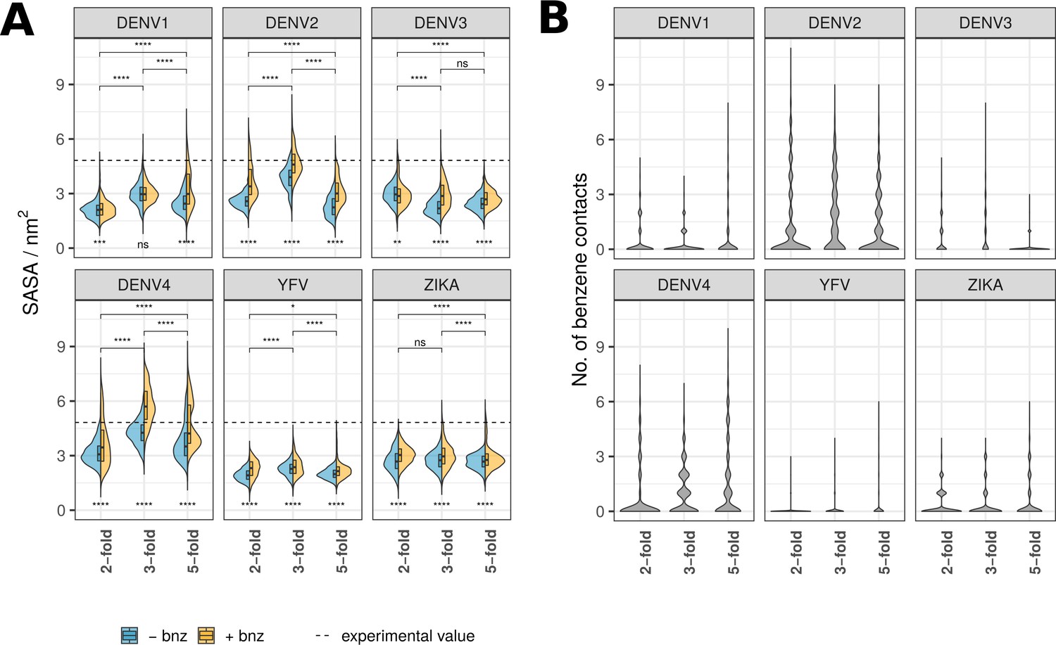
β-OG pocket properties of SASA and benzene contacts shown for individual viral strains and chain types.
(A) SASA calculated for β-OG pocket residues shown in split violin plots, where the blue area represents pocket SASA in water-only simulations, while the yellow surface represents simulations with benzene molecules present in the solvent. Experimental SASA value corresponds to the crystal structure pockets averaged across two chains. The division of pockets based on chain positions on the raft follows the labelling convention described in Figure 1A. Scores underneath the violin plots indicate the significance of SASA difference for water-only and benzene simulations. Pairwise scores above the plots describe a significant difference between chain types (across both solvent types). Significance is calculated using a Wilcoxon signed-rank test (ns: p>0.5; *: p≤0.5; **: p≤0.01; ***: p≤0.001; ****: p≤0.0001). (B) The number of benzene contacts occupying the β-OG pocket at any given point throughout the course of simulations. The values are shown for individual viruses and chain types.
Figure 5 with 1 supplement
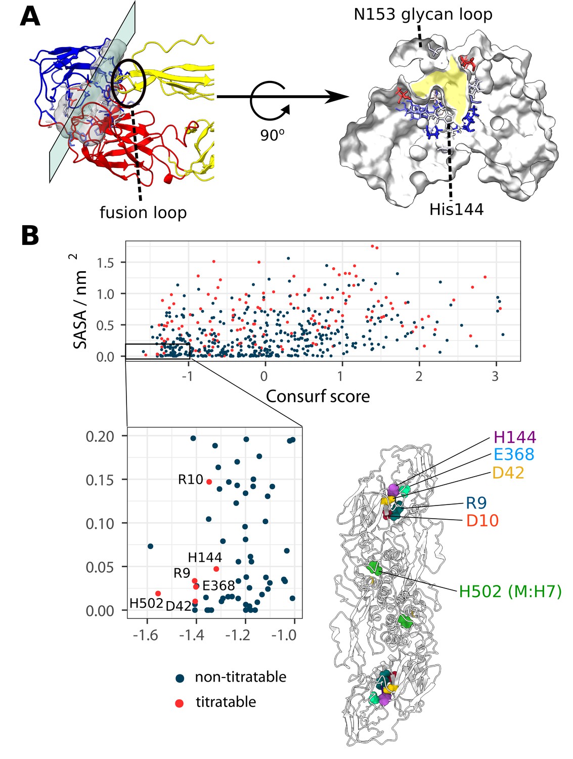
The location of the ⍺ pocket and the selection of all conserved, buried and titratable residues on the flaviviral envelope, showcasing a charge cluster associated with the pocket.
(A) Left side: The ⍺ pocket density displayed as a transparent grey surface located on the intrachain DI-DIII and interchain DII-DIII interface. The E protein is shown in ribbon representation and coloured according to domain assignments (as seen in Figure 1). The plane represents a directional slice of the pocket shown on the right side of the panel. Right side: The protein is shown in white surface representation and the residues lining the pocket are displayed as sticks and coloured according to their Consurf conservation score. The pocket is highlighted in yellow. (B) The selection of E and M protein residues according to the properties of conservation, burial, and ionizability. Residues characterised by a high degree of conservation (Consurf score ≤–1.0) and solvent inaccessibility (SASA ≤0.2 nm2) are shown in the inset. Additionally, titratable residues are labelled and displayed on the E2M2 structure, where it becomes apparent that almost all selected residues occupy the DI-DIII interface region associated with the ⍺ pocket. For ⍺ pocket SASA measurements across flaviviral strains, see Figure 5—figure supplement 1.
Figure 5—figure supplement 1
⍺ pocket SASA values across different viral strains and solvent compositions.
Grouping categories and the methods for calculating statistical significance are described in Figure 2A.
Figure 6 with 7 supplements
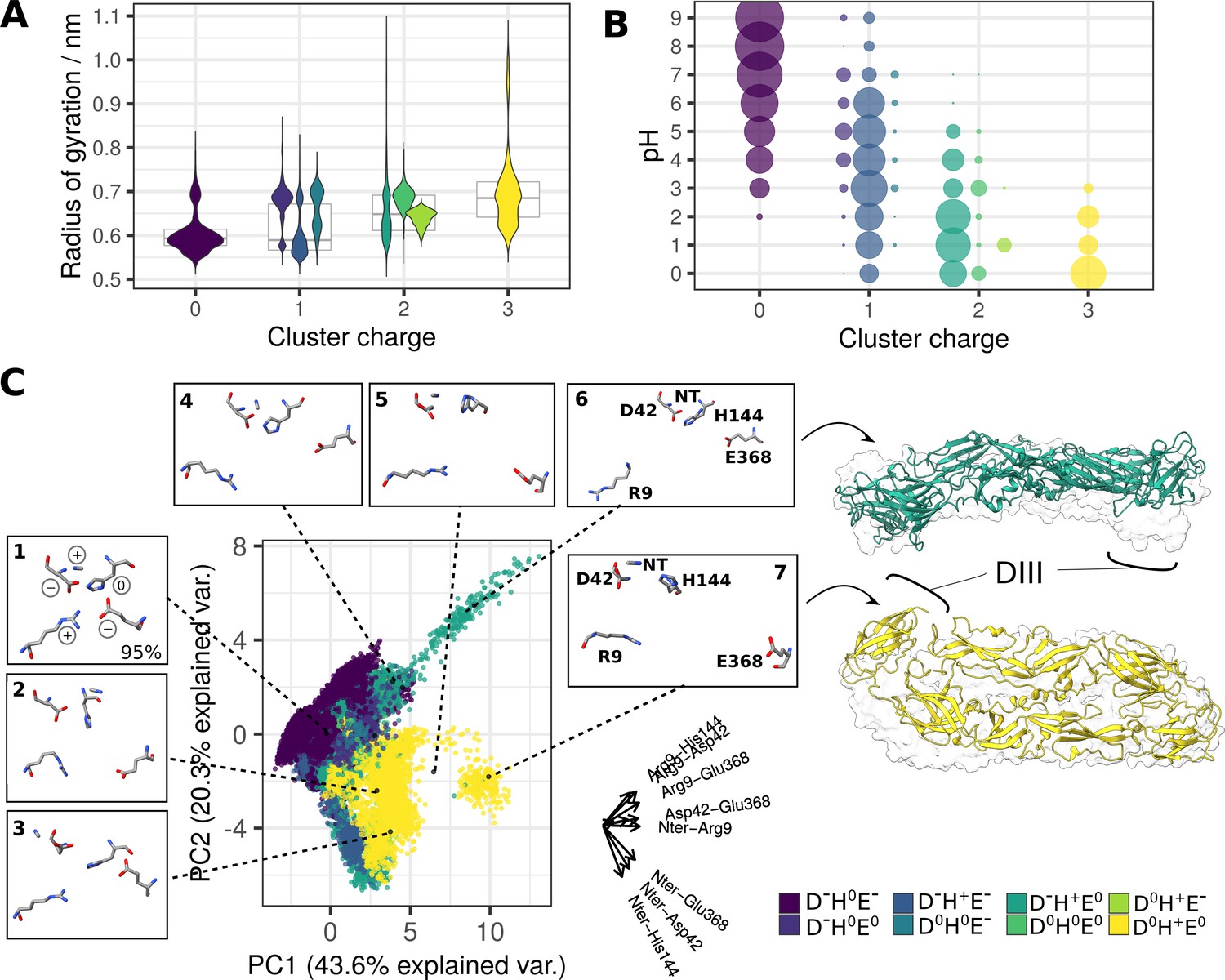
The response of the charge cluster to varying pH conditions.
For convergence of pKa values in constant-pH simulations, see Figure 6—figure supplement 1. (A) Disruption of the charge cluster (assessed via its radius of gyration) in relation to the charge pattern (violin plots in the foreground) and overall cluster charge (boxplots in the background). The measurements were obtained over a range of pH values (pH 0–9). The violin plots represent the distribution of y-values (radius of gyration measurements) for each protonation state, where the total area of violin(s) for each protonation state is constant. The codes in the legend describe residue charges for the residues that were titrated in the simulation system: Asp42, His144, and Glu368. N-ter and Arg9 had a fixed positive charge and were therefore omitted. For predicted pKa values of selected residues, see Figure 6—figure supplement 2. (B) Occurrence of distinct protonation states at different pH conditions. Point sizes correspond to the population sizes at each value. D-H0E- is a dominant pattern of charge in high and neutral pH conditions, whereas the remaining seven patterns (representing +1,+2, and+3 total cluster charge) appear at low pH conditions. See also Figure 6—figure supplement 3. (C) PCA describing cluster conformations based on the intra-cluster distances. The axes corresponding to the original variables are shown on the right side of the plot (labels for the smallest axes His144-Glu368 and Asp42-His144 omitted for clarity). Clustering analysis of the five residues (details in the Methods section) generated nine distinct conformations which are projected onto the PCA and shown in insets around the plot. Conformations 8 and 9 had a negligible contribution to the total number of structures and were therefore excluded from the visualisation. The snapshots corresponding to structures undergoing a greater conformational change at low pH are visualised in ribbon representation (trajectories shown in Figure 6—videos 1; 2). Transparent surfaces represent the starting sE dimer conformation, demonstrating the extent of the conformational shift. Ribbon colours correspond to the specific charge patterns under which the conformational change had occurred (green and yellow for D-H+E0 and D0H+E0, respectively). For SASA of the ⍺ pocket across different charge states of the cluster, see Figure 6—figure supplement 4. For the effects of benzene on the conserved cluster behaviour, see Figure 6—figure supplement 5.
Figure 6—figure supplement 1
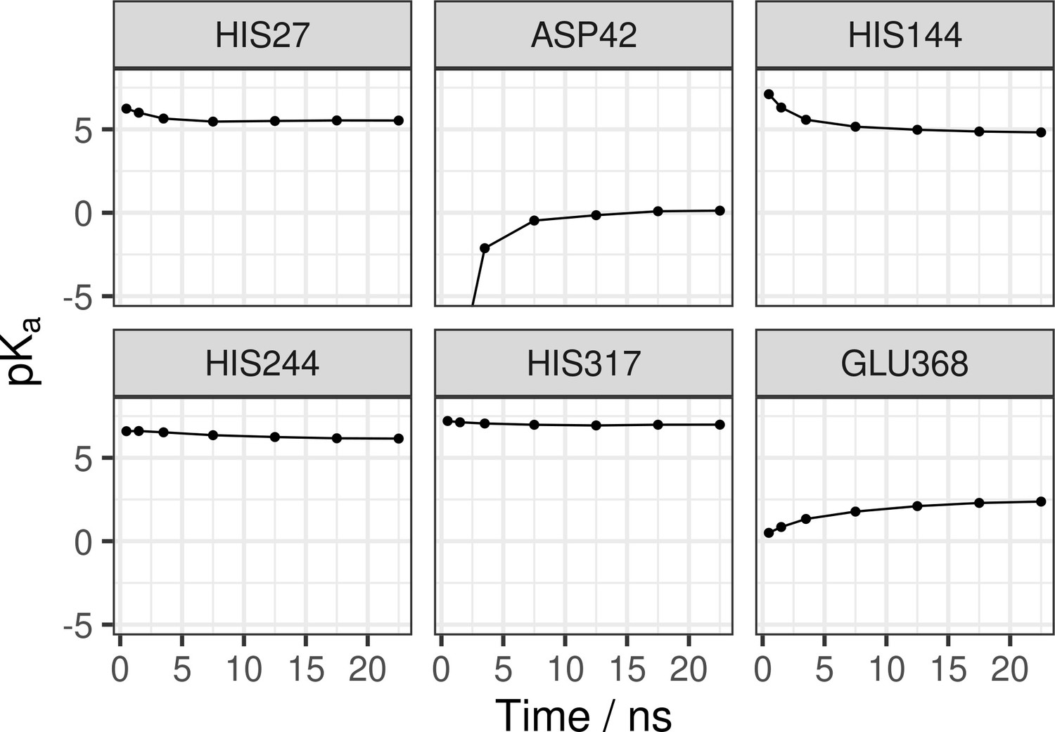
Convergence of pKa values.
pKas were calculated from a deprotonated fraction of each residue of interest and using the Hendersson-Hasselbalch equation. The pKas were calculated using progressively longer simulation times (1, 2, 5, 10, 15, and 20 ns, as well as the full-length trajectory). The pKa convergence is satisfied within ~5 ns of simulation, with buried residues (Asp42, His144, Glu368) converging more slowly as compared to the surface-exposed residues.
Figure 6—figure supplement 2
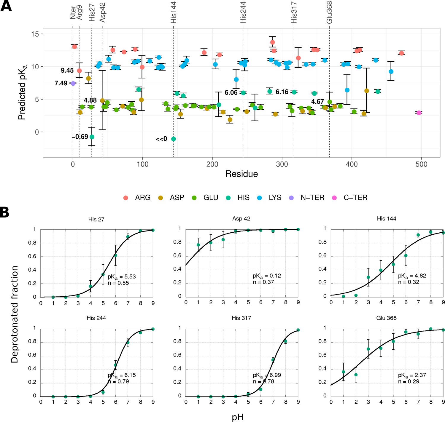
Prediction of pKa values for selected E protein residues using static structures and MD simulations.
(A) A pKa prediction for all titratable residues of the E protein calculated by the FD/DH method. The values are averaged across three chains in the asymmetric unit and standard errors are shown as whiskers. (B) Titration of selected residues derived from constant-pH simulations of the DENV2 sE dimer. The values are averaged across both chains and all repeats, with the standard errors shown as whiskers. The curves are fitted according to the Hill equation, where n is a Hill coefficient describing cooperativity between proton binding sites (n<1, negative cooperative binding; n=1, independent binding; n>1, positive cooperative binding).
Figure 6—figure supplement 3
Occurrence of conformations at different charge states.
Conformation 1 is predominant at all charge states, whereas other conformations are enriched at higher charges (+2 and+3) occurring at low pH. The labelled percentages describe the population proportion belonging to conformation 1.
Figure 6—figure supplement 4
⍺ pocket SASA values across different protonation states (violins) and charge states (boxplots) of the conserved cluster.
The SASA measurements were calculated from constant-pH simulations and across a range of pH values (pH 0–9). The violin plots (in the foreground) represent the distribution of SASA values for each protonation state, and the boxplots (in the background) show the distribution of SASA for each charge cluster. The codes in the legend are residue charges for the residues that were titrated in the simulation system (Asp42, His144, and Glu368).
Figure 6—figure supplement 5
Benzene contacts and its effects on the charge cluster.
(A) Number of benzene contacts for each residue within the cluster of charges (Nter-Arg9-Asp42-His144-Glu368) and across examined virus species. (B) The radius of gyration (measuring cluster disruption) in relation to the number of benzene molecules interacting with His144 across all examined flaviviruses. The increased number of benzene molecules within the ⍺ pocket leads to a greater disorder within the cluster. A point-to-point line connects the mean values of all groups (whereas boxplots highlight the median values of groups).
Figure 6—video 1
The top-down view of the DIII dissociation in DENV2 sE dimer under low pH conditions.
Figure 6—video 2
The side view of the DIII tilt in DENV2 sE dimer under low pH conditions.
Author response image 1
sE protein dimer capacitance as a function of pH.
The charge fluctuation was allowed on twelve residues of the simulation system (six on each monomer): His27, Asp42, His144, His244, His317, Glu368.
Tables
Table 1
Flaviviral envelope raft simulations in presence or absence of benzene in the simulation system.
| Strain | Solvent* | Time / ns | Repeats |
|---|---|---|---|
| DENV1-PVP159 | water | 300 | 3 |
| DENV1-PVP159 | 0.6 M benzene | 300 | 5 |
| DENV2-NGC | water | 300 | 3 |
| DENV2-NGC | 0.6 M benzene | 300 | 5 |
| DENV3-H87 | water | 300 | 3 |
| DENV3-H87 | 0.6 M benzene | 300 | 5 |
| DENV4-H241 | water | 300 | 3 |
| DENV4-H241 | 0.6 M benzene | 300 | 5 |
| YFV-17D | water | 300 | 3 |
| YFV-17D | 0.6 M benzene | 300 | 5 |
| ZIKA-H/PF/2013 | water | 300 | 3 |
| ZIKA-H/PF/2013 | 0.6 M benzene | 300 | 5 |
-
*
Both types of solvent contained charge-neutralising 0.15 M NaCl.
Additional files
Download links
A two-part list of links to download the article, or parts of the article, in various formats.
Downloads (link to download the article as PDF)
Open citations (links to open the citations from this article in various online reference manager services)
Cite this article (links to download the citations from this article in formats compatible with various reference manager tools)
A pH-dependent cluster of charges in a conserved cryptic pocket on flaviviral envelopes
eLife 12:e82447.
https://doi.org/10.7554/eLife.82447


