Figures and data in Quantifying how post-transcriptional noise and gene copy number variation bias transcriptional parameter inference from mRNA distributions

Figures
Tables
Additional files

15 figures, 16 tables and 1 additional file

Figures

Figure 1

Download asset Open asset

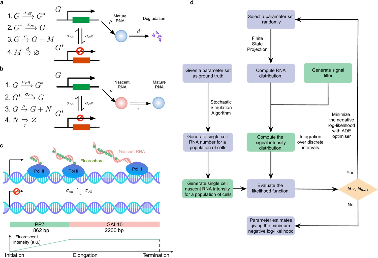
Overview of the inference of transcriptional parameters from synthetic data.

(a) A schematic illustration of the telegraph model. (b). A schematic of the delay telegraph model. The double horizontal line for nascent mRNA removal indicates this is a delayed reaction. (c) Illustration showing promoter switching between two states, Pol II binding to the promoter in the ON state and subsequently undergoing productive elongation. Note that the length of the nascent mRNA tail increases until Pol II terminates at the end of the gene. As Pol II travels through the 14 repeats of the PP7 loops, the intensity of the mRNA increases due to fluorescent probe binding to the mRNA; intensity saturates as Pol II enters the *GAL10* gene body. (d) Illustration of the algorithms to generate synthetic data and to perform inference from mature and nascent mRNA data. The green boxes are only applicable for the inference of the fluorescence signal intensity of nascent mRNAs; note that in nascent mRNA inference, the "RNA number" in the flow chart should be interpreted as the number of bound Pol II molecules on the gene. A large iteration step $N_{max}$ ( $\geq 10^{4}$ ) is chosen as the termination condition for the optimizer.

Figure 2

Download asset Open asset

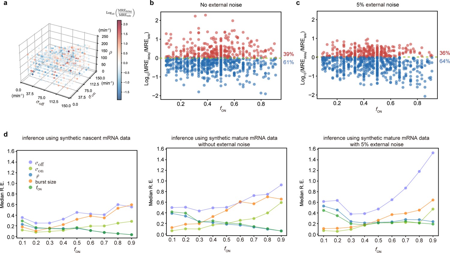
Accuracy of the inferred kinetic parameters from synthetic mature and nascent mRNA data using the telegraph and delay telegraph model, respectively.

(a) 3D scatter plot showing the ratio of the mean relative error from nascent mRNA data (using delay telegraph model ${MRE}_{delay}$ ) and the mean relative error from mature mRNA data (using the telegraph model ${MRE}_{tele}$ ) for 789 independent parameter sets sampled on a grid. Red data points indicate parameter sets with lower relative errors for mature data compared to nascent data, blue datapoints indicate parameter sets with lower relative error for nascent data compared to mature data (b) Same data as (a) but shown as a function of the fraction of ON time, $f_{ON}$ . For $\approx 61 %$ of the parameters, the inference accuracy is higher when using nascent mRNA data. (c) Sampling from the same parameter space, we then add log-normal distributed noise (size 5%) to the initiation rate $ρ$ (see text for details) to mimic external noise due to post-transcriptional processing that is only present in mature mRNA. Log₁₀ of the ratio of the median relative error (MRE) using perturbed mature mRNA data against Log₁₀ MRE using nascent mRNA data is shown as a function of the true fraction of ON time, $f_{ON}$ . For $\approx 64 %$ of the parameters, the inference accuracy is higher when using nascent mRNA data. (d) The median relative error of each transcriptional parameter as a function of the fraction of ON time, using synthetic nascent mRNA, synthetic mature mRNA data and synthetic mature mRNA with external noise. Inference from nascent data is generally more accurate than using mature mRNA data.

Figure 3

Download asset Open asset

Inference results using four mature mRNA data sets with sample sizes of 2333, 6366, 4550 and 3163 cells, respectively.

(a) Representative smFISH image of a yeast cell with *PP7-GAL10* RNAs labeled with Cy3 and the nucleus labeled with DAPI. (b) The DAPI and Cy3 signals were used to determine the nuclear and cellular mask, respectively. Detected and fitted spots are indicated in green. Mature RNA count distribution (pink) for segmentation method 1 with a best fit obtained from the telegraph model (gray curve). Scale bar is 5 μm(**c-d**) The DAPI and Cy3 signals were used to determine the nuclear and cellular mask using a second independent segmentation tool (segmentation 2). Mature RNA count distribution (gray and cyan) with/without counting the transcription site (TS) for segmentation method 2 with a best fit obtained from the telegraph model (gray curves). (e) Bar graphs of inferred transcriptional parameters (merged mature RNA data) from fitting the distributions of the two segmentation methods (‘seg1’ and ‘seg2’) as well as the distribution of mature RNAs only (‘seg2 -TS’ which indicates the exclusion of one spot in each cell that represents the transcription site). The burst size was computed as $ρ / σ_{off}$ and the fraction of ON time as $σ_{on} / (σ_{on} + σ_{off})$ . Error bars indicate standard deviation computed over the four datasets. (f) Distribution of the integrated DAPI intensity for each cell. Cyan line represents a Gaussian bimodal fit with highlighted regions indicating the intensity-based classification of G1 and G2 cells. Distributions of the mature RNA count for all cells (merged) and cell-cycle classified cells (G1 cells and G2 cells). (g) Tables and bar graphs of inferred parameters for merged and cell-cycle-specific data. Note that the transcriptional parameters $σ_{on}, σ_{off}, ρ$ are normalised by the degradation rate and hence dimensionless. For the cell-cycle-specific data, parameters were inferred per gene copy.

Figure 4

Download asset Open asset

Inference from the normalized nascent mRNA distributions for merged and cell-cycle specific data.

(a) Normalized nascent mRNA distributions of merged cell-cycle data were obtained by normalizing the signal intensity of the transcription site (defined as the brightest spot in the cell) by the median signal intensity of the cytoplasmic spots (shown in orange and zoom-in depicted in the inset). In all 4 datasets, approximately 90% of the detected cytoplasmic spots fell in the range 0.5× median – 1.5× median (grey bargraph). Black line in normalized distribution on the right represents best fit with delay telegraph model. (b) Nascent RNA distributions for cell-cycle-specific data. Black lines represent best fits with delay telegraph model. (c) Bar graphs comparing the transcriptional parameters, burst size, fraction of ON time and Fano factor for cell-cycle-specific and merged data. Error bars indicate standard deviation of the four datasets. (d) Normalized ACF plots of cell-cycle-specific and merged data. The ACF plots are generated by stochastic simulations using estimated parameters from merged and cell-cycle specific nascent mRNA data for each of the four data sets; these were compared with the ACF measured directly using live-cell data in Donovan et al., 2019 (green line). (e) The sum of squared ACF residuals of merged and cell-cycle-specific data from each dataset (this is the sum of squared deviations between the measured and estimated normalised ACF where the sum was calculated over all time points).

Figure 5

Download asset Open asset

Inference results using the rejection method.

(a) Nascent RNA distributions for cell-cycle-specific and merged data. Black lines represent best fits with delay telegraph model using the rejection method. (only the distributions for dataset #1 $k = 4$ are shown). (b) Estimated transcriptional parameters, burst size, fraction of ON time and Fano factor (mean values and standard deviation error bars of the four datasets) by rejecting the first $k$ bins with $k = 1, 2, 3, 4$ . The estimated parameters are listed in Appendix 4—table 3. (c) Normalized autocorrelation function (ACF) predicted by stochastic simulations using the estimated parameters (for $k = 4$ ) for each of the four data sets versus that measured directly using live-cell data (green line). (d) The sum of squared residuals of the ACF of cell-cycle-specific data from each dataset without/with rejection when $k = 4$ .

Figure 6

Download asset Open asset

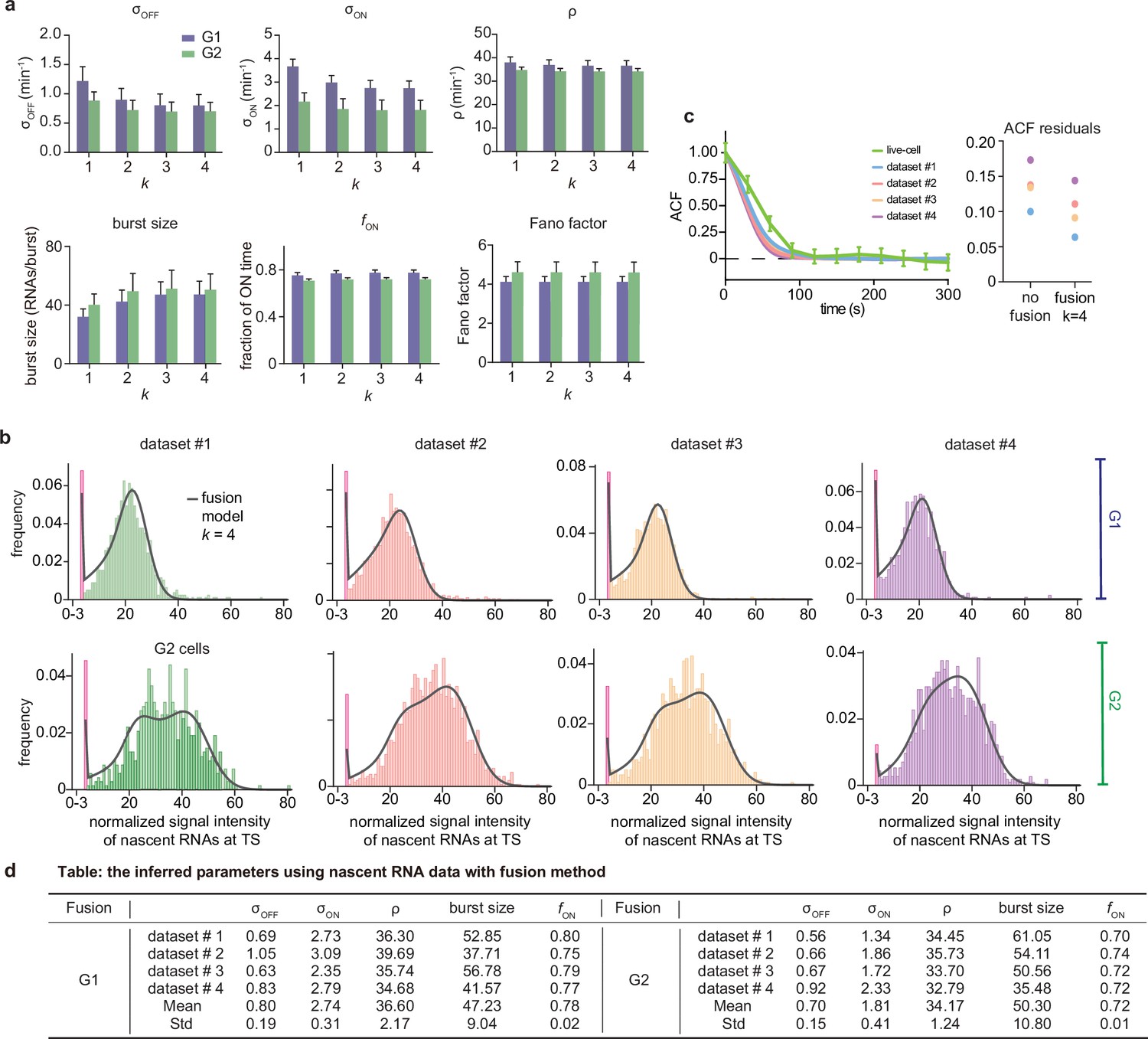
Inference results using the fusion method.

(a) Estimated burst size, fraction of ON and Fano factor (mean values and standard deviation error bars of the four datasets) by combining the first $k$ bins with $k = 1, 2, 3, 4$ . (b) Corresponding fitted distributions for G1 (top row) and G2 (bottom row) using delay telegraph model with the fusion method (only the distributions for $k = 4$ are shown). Magenta bar represents the combined bin 0–3 when $k = 4$ . (c) Normalised autocorrelation function (ACF) predicted by stochastic simulations using the estimated parameters (for $k = 4$ ) for each of the four data sets versus that measured directly using live-cell data (green line). The sum of squared residuals of the ACF plots using cell-cycle specific data without/with fusion method when $k = 4$ . (d) Estimated parameters of cell cycle specified data and merged data of nascent mRNAs with fusion method with $k = 4$ (fusing bins 0–3). These correspond to the fitted distributions in b. The elongation time $τ$ is fixed to 0.785 min. See the inferred parameters in Appendix 4—table 4 for all other values of $k$ .

Appendix 1—figure 1

Download asset Open asset

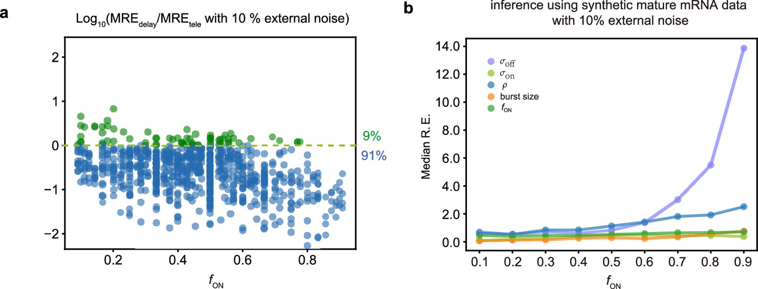
Comparing inference accuracy using synthetic nascent mRNA data and synthetic mature mRNA data with 10% external noise (log-normal distributed noise is added to the initiation rate $ρ$ to mimic external noise due to post-transcriptional processing that is only present in mature mRNA).

(a) Ratio of the mean relative errors in the two types of data as a function of the true fraction of ON time, $f_{ON}$ . For ≈91% (719/789) of the parameters, the inference accuracy is higher when using nascent mRNA data. (b) The median relative error of each transcriptional parameter as a function of the fraction of ON time using synthetic mature mRNA.

Appendix 1—figure 2

Download asset Open asset

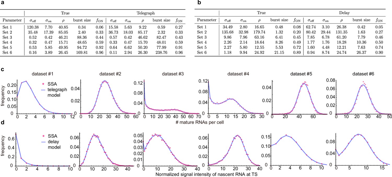
Inference with the telegraph model and delay telegraph model for six parameter sets.

(a) Estimates using the inference algorithm with the telegraph model (with no external noise) for six parameter sets. For both the ground truth and the estimated parameters, we fix the degradation rate $d = 1 {min}^{- 1}$ . (b). Estimates using the inference algorithm with the delay telegraph model for six parameter sets. For both the ground truth and the estimated parameters, we fix the delay $τ = 0.5 min$ . (c) Distributions from synthetic mature mRNA data fitted using the telegraph model. (d) Distributions from synthetic nascent mRNA data fitted using the delay telegraph model.

Appendix 2—figure 1

Download asset Open asset

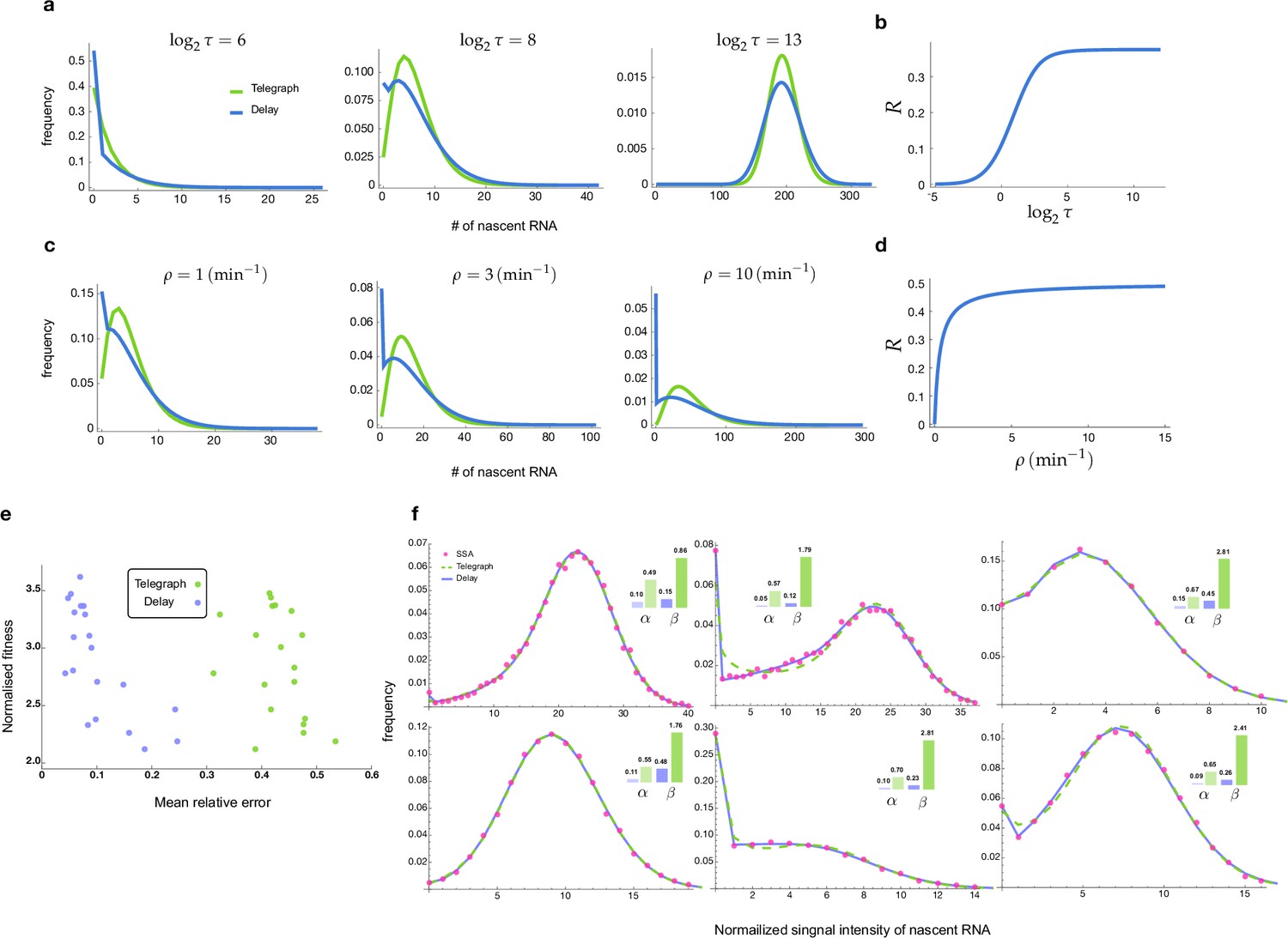
Distributions and mean errors of the transcriptional parameter inference.

(**a-d**) Comparison of the stochastic properties of the delay telegraph model and the telegraph model. a. Distributions of the nascent mRNA predicted by the delay telegraph model and the telegraph model for various values of $τ$ . We fix the parameters $(σ_{off}, σ_{on}, ρ) = (0.6, 0.03, 1)$ which implies that the change of $τ$ leads to a change in $x = τ (σ_{on} + σ_{off})$ at constant $y = (ρ / σ_{off}) {(σ_{off} / (σ_{off} + σ_{on}))}^{2}$ . (b) Corresponding relative error $R$ between the variances of two models calculated as a function of $τ$ using Equation (12). (c) Distributions of the nascent mRNA predicted by the delay telegraph model and the telegraph model for various values of $ρ$ . We fix the parameters $(σ_{off}, σ_{on}, τ) = (0.6, 0.03, 100)$ which implies that the change of $ρ$ leads to a change in $y$ at constant $x$ . (d) Corresponding relative error $R$ between the variances of two models calculated as a function of $ρ$ using Equation (12). (**e-f**) Inference of transcriptional parameters using as input synthetic fluorescent signal data generated by SSA simulations of transcription and fluorescent tagging for 10⁴ cells (see Methods section of the main text). (e) Mean relative error and normalised fitness score (fitness/number of samples) plot for 20 sets of numerical experiments. The inference is done in two different ways, using either the telegraph model (green) or the delayed telegraph model (blue). (f) Distributions of total fluorescent intensity from synthetic data (red dots) fit using the inference algorithm with telegraph model (dashed green) or delayed telegraph model (blue) for 6 different parameter sets. The insets show the relative errors in the estimates of the burst frequency ( $α$ ) and of the burst size ( $β$ ) calculated using Equation (13). Note that while both models provide a very good fit to the distribution from synthetic data, nevertheless parameter estimation is far more accurate using a delayed telegraph model. This is also reflected in (a) where we see low fitness scores for both models but a high mean relative error for estimates based on the telegraph model. The true and estimated parameters are shown in Appendix 2—table 1.

Appendix 3—figure 1

Download asset Open asset

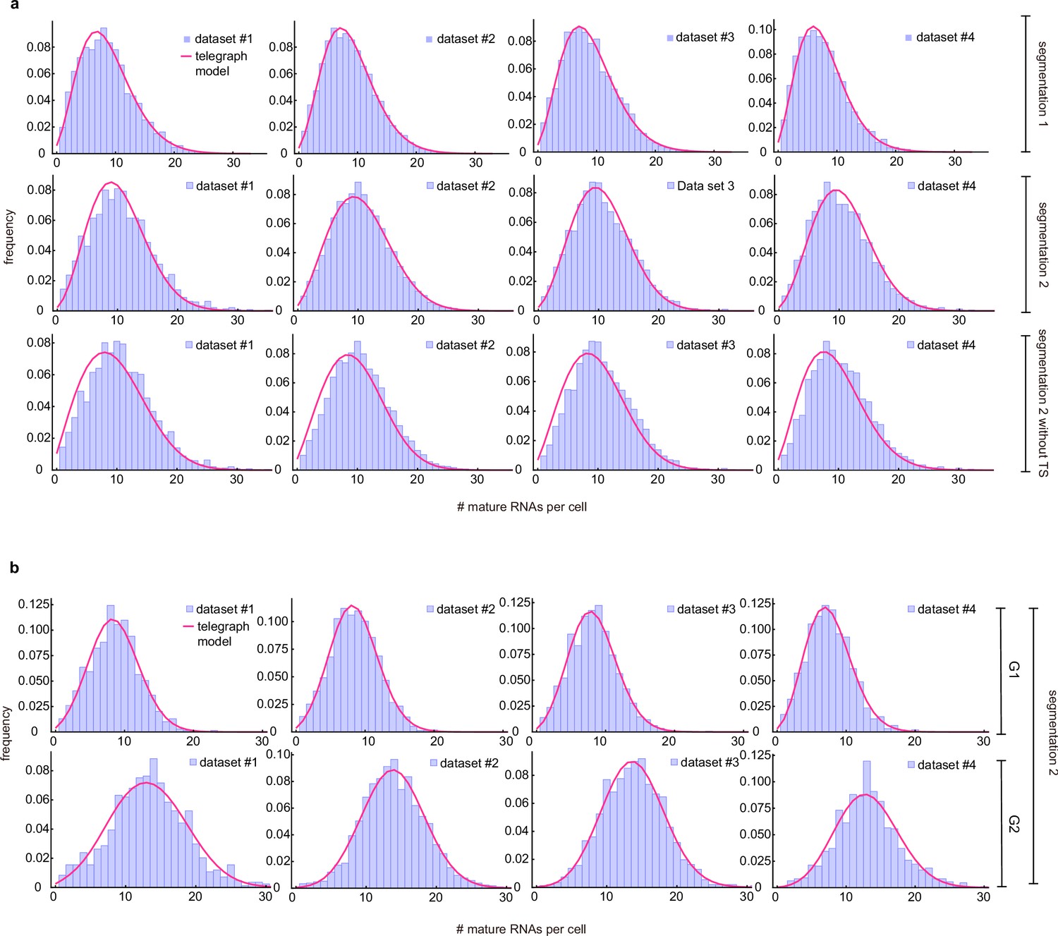
Merged and cell-cycle specific mature mRNA count distributions.

(a) Merged mature mRNA count distribution (purple) under segmentation method 1 and with/without counting the transcriptional site (TS) under segmentation method 2 with a best fit obtained from the telegraph model (magenta curves). (b) Cell-cyle specific mature mRNA count distribution (purple) under segmentation method 2 with a best fit obtained from the telegraph model (magenta curves).

Appendix 4—figure 1

Download asset Open asset

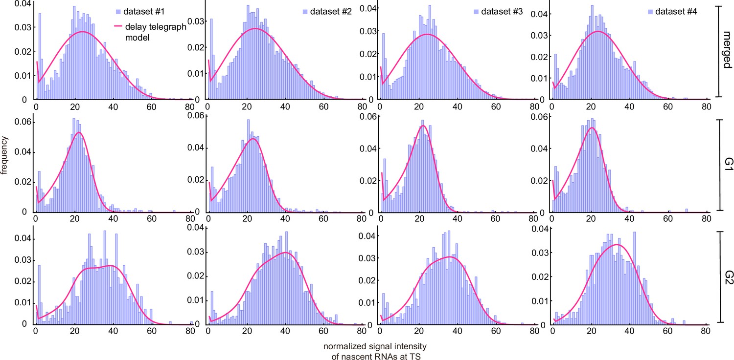
Inference results using merged and cell-cycle specific nascent data.

Experimental distributions (purple) are fit using the delay telegraph model (magenta curves).

Appendix 4—figure 2

Download asset Open asset

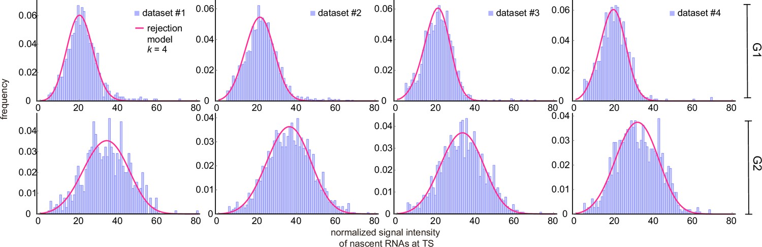
Inference results using cell-cycle specific data curated with the rejection method (only the distributions for $k = 4$ are shown).

Corresponding fitted distributions (purple) for G1 (top row) and G2 (bottom row) using the delay telegraph model (magenta curves).

Appendix 5—figure 1

Download asset Open asset

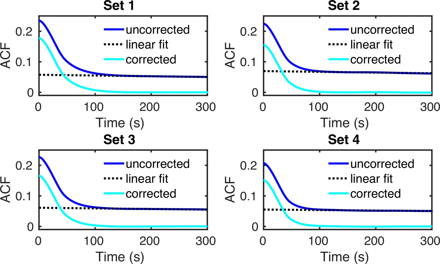
Autocorrelation functions of 10⁴ simulated *GAL10* intensity traces (solid blue lines).

The transcriptional parameters for G1 and G2 cells in the four sets of experimental data were obtained using the fusion method (see Figure 6d of the main manuscript). A linear fit (dashed black line) was subtracted to correct the ACFs for switching from G1 to G2 (solid cyan lines).

Appendix 6—figure 1

Download asset Open asset

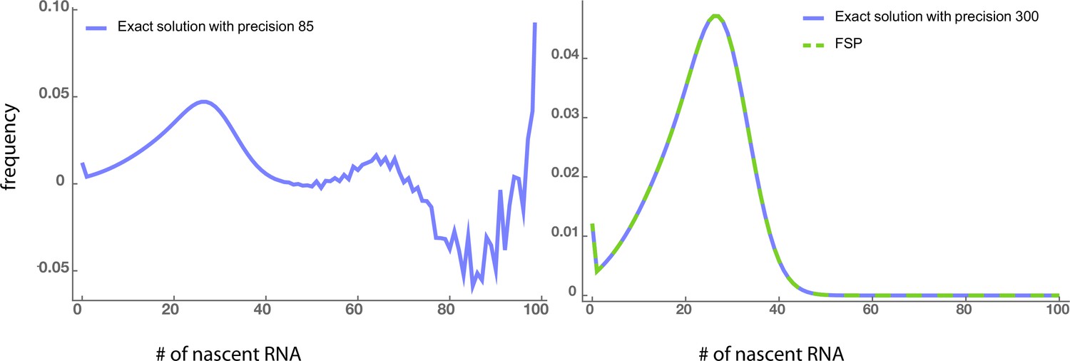
Left panel: Numerical instabilities due to the calculation of higher-order derivatives in the exact solution appear when the arithmetic precision is not very high (85).

Right panel: These instabilities disappear when the precision increases to 300. The exact solution with such high precision agrees well with the FSP method using double-precision floating-point (Float64) type. The parameters are, $σ_{off} = 1.71$ $σ_{on} = 5.82$ ,, $ρ = 53.74$ and. $τ = 0.56$

Appendix 7—figure 1

Download asset Open asset

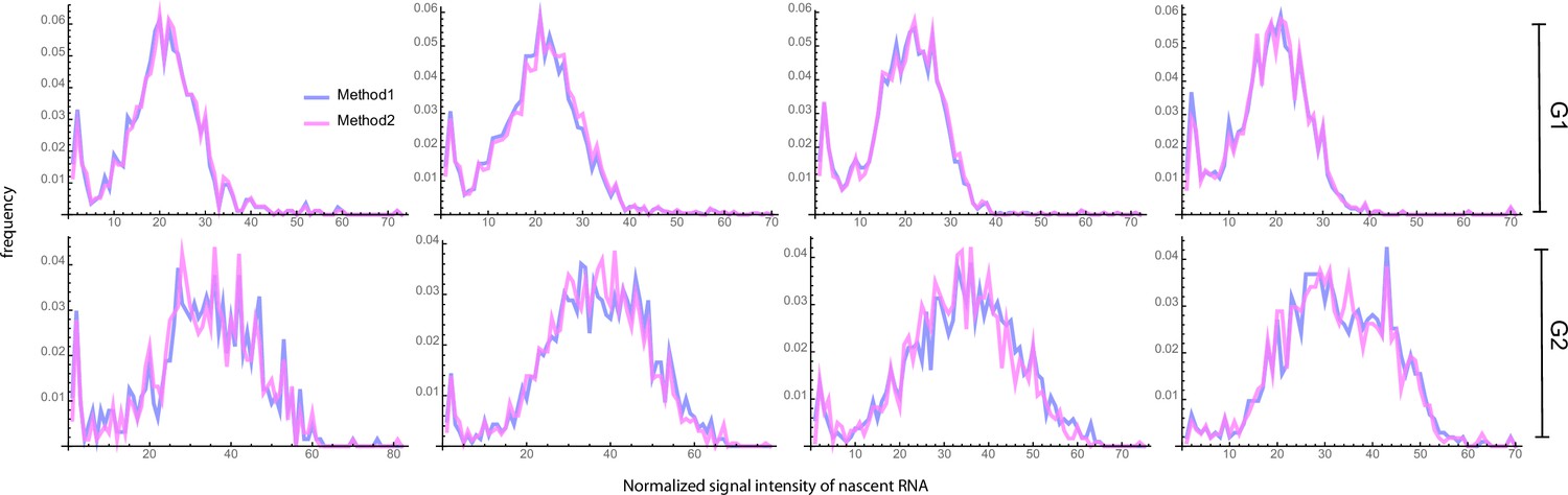
Blue curves (Method 1) show the fluorescent intensity distributions of the four experimental data sets after the classification of cells into G1 and G2 phases using the Fried/Baisch model.

Magenta curves (Method 2) show the same but using a bimodal Gaussian, as described in the main text.

Tables

Appendix 1—table 1

Mean and standard deviation of the parameters estimated from 10 independent synthetic datasets, generated for each parameter set in Appendix 1—figure 2.

Parameter	Mean					Standard deviation
Parameter	$σ_{off}$	$σ_{on}$	$ρ$	burst size	$f_{ON}$	$σ_{off}$	$σ_{on}$	$ρ$	burst size	$f_{ON}$
Set 1	31.85	2.69	15.68	0.53	0.10	19.07	0.22	7.68	0.07	0.05
Set 2	92.67	30.47	141.42	1.56	0.25	23.76	1.51	21.61	0.14	0.04
Set 3	9.94	8.01	63.35	6.39	0.45	0.72	0.19	1.94	0.25	0.01
Set 4	2.30	2.16	18.76	8.17	0.48	0.12	0.05	0.31	0.31	0.01
Set 5	2.26	5.80	12.57	5.59	0.72	0.19	0.30	0.11	0.41	0.01
Set 6	1.22	10.01	24.97	20.53	0.89	0.10	0.43	0.16	1.65	0.01

Appendix 1—table 2

95% confidence intervals of the 12 parameter sets (shown in Appendix 1—figure 2a-b).

Parameter	Telegraph CI			Delay CI
Parameter	$σ_{off}$	$σ_{on}$	$ρ$	$σ_{off}$	$σ_{on}$	$ρ$
Set 1	(6.76, 300.00)	(3.53, 8.49)	(5.59, 107.67)	(13.80, 300.00)	(1.85, 2.69)	(9.94, 160.51)
Set 2	(17.22, 190.38)	(14.56, 23.92)	(61.14, 250.51)	(103.80, 268.35)	(30.00, 35.38)	(161.54, 300.00)
Set 3	(0.54, 0.59)	(0.41, 0.43)	(46.08, 47.15)	(6.83, 8.55)	(6.42, 7.04)	(58.28, 63.18)
Set 4	(0.31, 0.35)	(0.46, 0.49)	(15.50, 15.91)	(1.64,1.99)	(1.65,1.85)	(17.92,18.77)
Set 5	(0.49, 0.85)	(5.82, 7.62)	(49.62, 50.92)	(1.56,2.59)	(4.58,5.85)	(12.08,12.97)
Set 6	(0.08, 0.16)	(2.46, 3.54)	(26.10, 26.54)	(0.73,1.24)	(7.53,9.75)	(24.32,25.14)

Appendix 1—table 3

Table showing the relative error against profile likelihood error of 12 parameter sets (shown in Appendix 1—figure 2a and b).

See text for details.

	Telegraph						Delay
	Relative error			Profile likelihood error			Relative error			Profile likelihood error
	$σ_{off}$	$σ_{on}$	$ρ$	$σ_{off}$	$σ_{on}$	$ρ$	$σ_{off}$	$σ_{on}$	$ρ$	$σ_{off}$	$σ_{on}$	$ρ$
Set 1	0.87	0.27	0.77	18.82	0.88	11.07	0.82	0.11	0.58	1.75	0.34	1.82
Set 2	0.04	0.04	1.44E-03	4.72	0.52	2.22	0.41	0.11	0.27	0.81	0.16	0.55
Set 3	0.08	0.01	0.01	0.09	0.06	0.02	0.20	0.15	0.03	0.22	0.09	0.08
Set 4	0.01	0.01	1.11E-03	0.14	0.07	0.03	0.22	0.18	0.02	0.20	0.11	0.05
Set 5	0.22	0.13	4.97E-03	0.55	0.27	0.03	0.30	0.23	0.03	0.64	0.28	0.07
Set 6	0.29	0.24	0.01	0.74	0.37	0.02	0.20	0.12	0.01	0.55	0.25	0.03

Appendix 1—table 4

Effects of random perturbations on inference of parameters from mature mRNA data (using the telegraph model).

Parameter	True					Unperturbed					–1/0/+1 stochastic perturbation
Parameter	$σ_{off}$	$σ_{on}$	$ρ$	burst size	$f_{ON}$	$σ_{off}$	$σ_{on}$	$ρ$	burst size	$f_{ON}$	$σ_{off}$	$σ_{on}$	$ρ$	burst size	$f_{ON}$
Set 1	120.38	7.70	40.85	0.34	0.06	15.58	5.63	9.22	0.59	0.27	0.59	1.17	3.70	6.28	0.66
Set 2	35.48	17.39	85.05	2.40	0.33	36.73	18.03	85.17	2.32	0.33	24.13	15.79	70.89	2.94	0.40
Set 3	0.52	0.42	46.21	88.36	0.44	0.57	0.42	46.62	82.47	0.43	0.61	0.46	47.17	76.74	0.43
Set 4	0.32	0.47	15.71	48.65	0.59	0.33	0.47	15.70	48.01	0.59	0.39	0.54	16.09	41.17	0.58
Set 5	0.53	5.85	49.95	94.72	0.92	0.64	6.62	50.20	77.99	0.91	0.68	6.72	50.35	74.48	0.91
Set 6	0.16	3.89	26.45	169.81	0.96	0.11	2.94	26.30	238.76	0.96	0.13	3.06	26.42	203.20	0.96

Appendix 1—table 5

Inference using the delay telegraph model from synthetic nascent fluorescent data, with and without perturbation by log-normal noise.

Parameter	True					Delay					Perturbation
Parameter	$σ_{off}$	$σ_{on}$	$ρ$	burst size	$f_{ON}$	$σ_{off}$	$σ_{on}$	$ρ$	burst size	$f_{ON}$	$σ_{off}$	$σ_{on}$	$ρ$	burst size	$f_{ON}$
Set 1	34.49	2.80	16.65	0.48	0.08	62.74	3.10	26.38	0.42	0.05	50.08	1.52	31.71	0.63	0.03
Set 2	135.68	32.98	179.74	1.32	0.20	80.42	29.44	131.35	1.63	0.27	233.96	30.74	300.00	1.28	0.12
Set 3	9.86	7.96	63.16	6.41	0.45	7.85	6.78	61.20	7.79	0.46	8.85	6.63	65.49	7.40	0.43
Set 4	2.26	2.14	18.64	8.26	0.49	1.77	1.76	18.28	10.36	0.50	1.90	1.64	18.65	9.83	0.46
Set 5	2.27	5.80	12.55	5.53	0.72	1.60	4.48	12.21	7.63	0.74	2.59	4.79	13.27	5.13	0.65
Set 6	1.18	9.94	24.92	21.15	0.89	0.94	8.74	24.74	26.37	0.90	1.84	10.15	26.10	14.18	0.85

Appendix 2—table 1

Estimates using the inference algorithm with delay telegraph and telegraph models for the six parameter sets in Appendix 2—figure 1f.

Parameter	True					Delay					Telegraph
Parameter	$σ_{off}$	$σ_{on}$	$ρ$	burst size	$f_{ON}$	$σ_{off}$	$σ_{on}$	$ρ$	burst size	$f_{ON}$	$σ_{off}$	$σ_{on}$	$ρ$	burst size	$f_{ON}$
Set 1	1.05	8.20	57.99	55.09	0.89	0.94	7.19	57.92	61.87	0.88	0.60	4.10	59.51	99.42	0.87
Set 2	1.27	3.14	58.17	45.69	0.71	1.13	2.91	58.01	51.16	0.72	0.45	1.22	59.43	133.07	0.73
Set 3	2.27	5.80	12.55	5.53	0.72	1.60	4.48	12.21	7.63	0.74	0.59	1.71	12.09	20.61	0.74
Set 4	1.18	9.94	24.92	21.15	0.89	0.94	8.74	24.74	26.37	0.90	0.46	4.12	24.92	54.00	0.90
Set 5	2.26	2.14	18.64	8.26	0.49	1.77	1.76	18.28	10.36	0.50	0.54	0.58	17.60	32.59	0.52
Set 6	1.38	4.77	21.74	15.79	0.78	1.08	4.00	21.50	19.94	0.79	0.38	1.49	21.31	56.44	0.80

Appendix 3—table 1

Inferred transcriptional parameters using merged mature mRNA data from segmentation 1, segmentation 2 and segmentation 2 without transcriptional site (TS).

Parameter	segmentation 1					segmentation 2					segmentation 2 without TS
Parameter	$σ_{off}$	$σ_{on}$	$ρ$	burst size	$f_{ON}$	$σ_{off}$	$σ_{on}$	$ρ$	burst size	$f_{ON}$	$σ_{off}$	$σ_{on}$	$ρ$	burst size	$f_{ON}$
Set 1	21.18	4.73	47.15	2.23	0.18	3.27	3.36	20.62	6.31	0.51	2.92	2.45	21.05	7.22	0.46
Set 2	19.53	5.44	40.11	2.05	0.22	3.22	3.87	19.17	5.95	0.55	2.46	2.68	18.35	7.46	0.52
Set 3	16.53	4.77	39.48	2.39	0.22	3.67	4.05	20.09	5.47	0.52	3.00	2.87	19.73	6.57	0.49
Set 4	28.72	5.16	50.00	1.74	0.15	5.79	4.58	23.04	3.98	0.44	5.27	3.27	24.33	4.61	0.38
Mean	21.49	5.02	44.19	2.10	0.19	3.99	3.97	20.73	5.43	0.50	3.41	2.82	20.87	6.46	0.46
Std	5.19	0.34	5.21	0.28	0.03	1.06	0.43	1.43	0.89	0.04	1.26	0.35	2.56	1.29	0.06

Appendix 3—table 2

95% confidence interval intervals for the estimates from experimental mature mRNA data using segmentation 2.

mature		$σ_{off}$	$σ_{on}$	$ρ$	CI for $σ_{off}, σ_{on}, ρ$
merged	Set 1	3.27	3.36	20.62	(2.08, 6.08)	(2.81, 4.16)	(18.03, 25.97)
	Set 2	3.22	3.87	19.17	(2.38, 4.69)	(3.41, 4.44)	(17.51, 21.62)
	Set 3	3.67	4.05	20.09	(2.54, 5.92)	(3.51, 4.79)	(18.03, 23.67)
	Set 4	5.79	4.58	23.04	(3.33, 13.33)	(3.79, 5.85)	(19.36, 33.51)
G1	Set 1	0.69	2.76	10.71	(0.27, 2.35)	(1.73, 4.96)	(9.77, 12.85)
	Set 2	0.60	2.80	10.27	(0.35, 1.24)	(2.13, 3.92)	(9.77, 11.15)
	Set 3	0.88	3.41	10.33	(0.38, 2.84)	(2.23, 5.77)	(9.58, 12.35)
	Set 4	2.46	5.21	11.12	(0.46, 300.00)	(2.68, 18.86)	(8.96, 216.67)
G2	Set 1	0.42	0.99	9.45	(0.22, 0.91)	(0.65, 1.48)	(8.64, 10.86)
	Set 2	0.14	1.01	7.92	(0.05, 0.36)	(0.56, 1.72)	(7.61, 8.46)
	Set 3	0.18	1.24	7.91	(0.05, 0.72)	(0.57, 2.59)	(7.49, 8.85)
	Set 4	0.42	1.68	8.19	(0.12, 2.07)	(0.76, 3.50)	(7.41, 10.28)

Appendix 3—table 3

Inferred transcriptional rate (normalized) per gene copy for the G2 cell cycle phase under the assumption that the two gene states are perfectly synchronized.

mature		$σ_{off}$	$σ_{on}$	$ρ$	burst size	$f_{ON}$
G2 sync	Set 1	0.62	2.17	8.45	13.69	0.78
	Set 2	0.37	3.26	7.72	21.05	0.90
	Set 3	0.67	4.42	7.92	11.85	0.87
	Set 4	0.55	3.45	7.55	13.62	0.86
	Mean	0.55	3.32	7.91	15.05	0.85
	Std	0.13	0.92	0.39	4.09	0.05

Appendix 4—table 1

Estimated parameters from the non-curated distribution of the normalized intensity of the brightest nuclear spot (nascent mRNA data) constructed by merging all data or else specific to the cell cycle phases G1 and G2.

The elongation time $τ$ is estimated to be 0.785 min, based on measurements of the elongation speed.

nascent		$σ_{off}$	$σ_{on}$	$ρ$	burst size	$f_{ON}$
merged	Set 1	5.24	5.07	77.46	14.78	0.49
	Set 2	5.58	5.13	82.11	14.71	0.48
	Set 3	5.11	5.17	76.09	14.90	0.50
	Set 4	5.96	6.13	73.23	12.30	0.51
	Mean	5.47	5.37	77.22	14.17	0.50
	Std	0.38	0.50	3.70	1.25	0.01
G1	Set 1	1.11	3.76	37.83	34.10	0.77
	Set 2	1.53	3.94	41.33	27.06	0.72
	Set 3	0.95	3.23	36.79	38.56	0.77
	Set 4	1.28	3.76	36.04	28.09	0.75
	Mean	1.22	3.67	38.00	31.95	0.75
	Std	0.25	0.31	2.34	5.39	0.02
G2	Set 1	0.74	1.69	35.00	47.30	0.70
	Set 2	0.82	2.18	36.30	44.37	0.73
	Set 3	0.91	2.19	34.54	37.90	0.71
	Set 4	1.08	2.61	33.27	30.76	0.71
	Mean	0.89	2.17	34.78	40.08	0.71
	Std	0.15	0.38	1.25	7.35	0.01

Appendix 4—table 2

95% confidence intervals for non-curated data estimated using the profile likelihood method.

nascent		$σ_{off}$	$σ_{on}$	$ρ$	burst size	$f_{ON}$	CI for $σ_{off}, σ_{on}, ρ$
merged	Set 1	5.24	5.07	77.46	14.78	0.49	(4.42, 6.23)	(4.68, 5.45)	(73.48, 82.92)
	Set 2	5.58	5.13	82.11	14.71	0.48	(5.05, 6.15)	(4.97, 5.37)	(79.38, 85.53)
	Set 3	5.11	5.17	76.09	14.90	0.50	(4.53, 5.71)	(4.98, 5.38)	(73.49, 79.64)
	Set 4	5.96	6.13	73.23	12.30	0.51	(5.19, 7.22)	(5.87, 6.57)	(69.34, 78.37)
G1	Set 1	1.11	3.76	37.83	34.10	0.77	(0.77, 1.66)	(3.04, 4.63)	(36.26, 39.96)
	Set 2	1.53	3.94	41.33	27.06	0.72	(1.29, 1.88)	(3.64, 4.40)	(40.18, 42.85)
	Set 3	0.95	3.23	36.79	38.56	0.77	(0.77, 1.17)	(2.86, 3.60)	(36.05, 37.69)
	Set 4	1.28	3.76	36.04	28.09	0.75	(0.99, 1.73)	(3.18, 4.34)	(34.68, 37.75)
G2	Set 1	0.74	1.69	35.00	47.30	0.70	(0.54, 1.02)	(1.36, 2.08)	(33.64, 36.72)
	Set 2	0.82	2.18	36.30	44.37	0.73	(0.66, 1.07)	(1.85, 2.52)	(35.35, 37.40)
	Set 3	0.91	2.19	34.54	37.90	0.71	(0.70, 1.23)	(1.85, 2.61)	(33.38, 36.05)
	Set 4	1.08	2.61	33.27	30.76	0.71	(0.75, 1.71)	(2.00, 3.41)	(31.91, 35.40)

Appendix 4—table 3

(Rejection method) Estimated parameters by discarding the first $k$ signal bins of the experimental distribution of the signal intensity (and renormalizing afterwards).

Inference is done for each of the four data sets. The elongation time is fixed to $τ \approx 0.785$ min.

k = 1		$σ_{off}$	$σ_{on}$		burst size	$f_{O N}$
G1	Set 1	1.06	4.33	36.62	34.63	0.80
	Set 2	1.45	4.42	39.84	27.51	0.75
	Set 3	1.04	3.84	36.66	35.19	0.79
	Set 4	1.27	4.12	35.41	27.78	0.76
	Mean	1.21	4.18	37.13	31.28	0.78
	Std	0.19	0.26	1.90	4.20	0.02
G2	Set 1	0.84	2.10	34.54	41.20	0.71
	Set 2	0.97	2.94	35.49	36.73	0.75
	Set 3	0.94	2.53	33.68	35.99	0.73
	Set 4	1.20	3.07	32.81	27.28	0.72
	Mean	0.99	2.66	34.13	35.30	0.73
	Std	0.15	0.44	1.15	5.82	0.02
$k = 2$		$σ_{off}$	$σ_{on}$	$ρ$	burst size	$f_{ON}$
G1	Set 1	1.58	6.33	37.77	23.89	0.80
	Set 2	1.93	5.93	40.86	21.16	0.75
	Set 3	1.28	5.15	37.07	29.07	0.80
	Set 4	1.55	5.29	35.92	23.10	0.77
	Mean	1.59	5.67	37.91	24.30	0.78
	Std	0.27	0.55	2.11	3.38	0.02
G2	Set 1	1.43	3.42	35.83	25.11	0.71
	Set 2	1.69	4.39	37.42	22.10	0.72
	Set 3	1.33	3.38	34.64	26.08	0.72
	Set 4	1.56	3.68	33.70	21.61	0.70
	Mean	1.50	3.72	35.39	23.72	0.71
	Std	0.16	0.47	1.61	2.20	0.01
$k = 3$		$σ_{off}$	$σ_{on}$	$ρ$	burst size	$f_{ON}$
G1	Set 1	2.66	9.03	39.73	14.92	0.77
	Set 2	2.55	7.41	42.04	16.46	0.74
	Set 3	1.64	6.67	37.69	22.92	0.80
	Set 4	2.22	7.32	37.02	16.65	0.77
	Mean	2.27	7.61	39.12	17.73	0.77
	Std	0.46	1.00	2.26	3.54	0.02
G2	Set 1	2.01	4.35	37.23	18.50	0.68
	Set 2	2.16	5.10	38.56	17.85	0.70
	Set 3	1.70	4.05	35.55	20.85	0.70
	Set 4	1.88	4.16	34.48	18.30	0.69
	Mean	1.94	4.41	36.45	18.88	0.69
	Std	0.19	0.48	1.80	1.34	0.01
$k = 4$		$σ_{off}$	$σ_{on}$	$ρ$	burst size	$f_{ON}$
G1	Set 1	6.10	14.18	44.41	7.28	0.70
	Set 2	3.72	9.57	43.96	11.81	0.72
	Set 3	2.02	7.99	38.25	18.89	0.80
	Set 4	2.75	8.60	37.78	13.76	0.76
	Mean	3.65	10.09	41.10	12.94	0.74
	Std	1.77	2.80	3.57	4.81	0.04
G2	Set 1	2.12	4.50	37.48	17.68	0.68
	Set 2	2.59	5.68	39.55	15.25	0.69
	Set 3	2.47	5.14	37.27	15.08	0.68
	Set 4	2.18	4.55	35.17	16.13	0.68
	Mean	2.34	4.97	37.37	16.04	0.68
	Std	0.23	0.56	1.79	1.19	0.01

Appendix 4—table 4

(Fusion method) Estimated parameters by combining the first $k$ signal bins of the experimental distribution of the signal intensity.

Inference is done for each of the four data sets. The elongation time is fixed to $τ \approx 0.785$ min.

$k = 1$		$σ_{off}$	$σ_{on}$	$ρ$	burst size	$f_{ON}$
G1	Set 1	1.11	3.76	37.83	34.10	0.77
	Set 2	1.53	3.94	41.33	27.06	0.72
	Set 3	0.95	3.23	36.79	38.56	0.77
	Set 4	1.28	3.76	36.04	28.09	0.75
	Mean	1.22	3.67	38.00	31.95	0.75
	Std	0.25	0.31	2.34	5.39	0.02
G2	Set 1	0.74	1.69	35.00	47.30	0.70
	Set 2	0.82	2.18	36.30	44.37	0.73
	Set 3	0.91	2.19	34.54	37.90	0.71
	Set 4	1.08	2.61	33.27	30.76	0.71
	Mean	0.89	2.17	34.78	40.08	0.71
	Std	0.15	0.38	1.25	7.35	0.01
$k = 2$		$σ_{off}$	$σ_{on}$	$ρ$	burst size	$f_{ON}$
G1	Set 1	0.78	2.99	36.65	46.99	0.79
	Set 2	1.14	3.27	40.01	35.06	0.74
	Set 3	0.71	2.58	36.00	51.00	0.79
	Set 4	0.96	3.09	35.08	36.52	0.76
	Mean	0.90	2.98	36.94	42.39	0.77
	Std	0.19	0.30	2.15	7.82	0.02
G2	Set 1	0.54	1.30	34.37	63.20	0.70
	Set 2	0.67	1.87	35.74	53.70	0.74
	Set 3	0.74	1.88	33.96	45.75	0.72
	Set 4	0.94	2.36	32.84	34.89	0.72
	Mean	0.72	1.85	34.23	49.38	0.72
	Std	0.17	0.44	1.20	12.01	0.01
$k = 3$		$σ_{off}$	$σ_{on}$	$ρ$	burst size	$f_{ON}$
G1	Set 1	0.71	2.79	36.38	51.39	0.80
	Set 2	1.07	3.14	39.77	37.01	0.75
	Set 3	0.63	2.35	35.74	56.84	0.79
	Set 4	0.80	2.71	34.58	43.09	0.77
	Mean	0.80	2.75	36.62	47.08	0.78
	Std	0.19	0.32	2.23	8.78	0.02
G2	Set 1	0.52	1.25	34.30	65.86	0.71
	Set 2	0.65	1.84	35.70	54.75	0.74
	Set 3	0.71	1.81	33.85	47.67	0.72
	Set 4	0.91	2.31	32.76	35.91	0.72
	Mean	0.70	1.80	34.15	51.05	0.72
	Std	0.16	0.43	1.22	12.57	0.01
$k = 4$		$σ_{off}$	$σ_{on}$	$ρ$	burst size	$f_{ON}$
G1	Set 1	0.69	2.73	36.30	52.85	0.80
	Set 2	1.05	3.09	39.69	37.71	0.75
	Set 3	0.63	2.35	35.74	56.78	0.79
	Set 4	0.83	2.79	34.68	41.57	0.77
	Mean	0.80	2.74	36.60	47.23	0.78
	Std	0.19	0.31	2.17	9.04	0.02
G2	Set 1	0.56	1.34	34.45	61.05	0.70
	Set 2	0.66	1.86	35.73	54.11	0.74
	Set 3	0.67	1.72	33.70	50.56	0.72
	Set 4	0.92	2.33	32.79	35.48	0.72
	Mean	0.70	1.81	34.17	50.30	0.72
	Std	0.15	0.41	1.24	10.80	0.01

Appendix 4—table 5

Inference of the kinetic parameters $(σ_{off}, σ_{on}, ρ)$ using nascent data curated with the fusion method.

Inferred values and the corresponding 95% confidence intervals of G1 and G2 cell-cycle-specific data calculated using the profile likelihood method.

nascent		$σ_{off}$	$σ_{on}$	$ρ$	burst size	$f_{ON}$	CI for $σ_{off}, σ_{on}, ρ$
G1	Set 1	0.69	2.73	36.30	52.85	0.80	(0.46, 1.05)	(2.12, 3.52)	(35.06, 37.91)
	Set 2	1.05	3.09	39.69	37.71	0.75	(0.86, 1.29)	(2.73, 3.47)	(38.77, 40.92)
	Set 3	0.63	2.35	35.74	56.78	0.79	(0.49, 0.79)	(1.99, 2.71)	(35.06, 36.58)
	Set 4	0.83	2.79	34.68	41.57	0.77	(0.62, 1.16)	(2.27, 3.41)	(33.54, 36.01)
G2	Set 1	0.56	1.34	34.45	61.05	0.70	(0.40, 0.81)	(1.04, 1.73)	(33.35, 35.82)
	Set 2	0.66	1.86	35.73	54.11	0.74	(0.51, 0.85)	(1.57, 2.21)	(34.87, 36.77)
	Set 3	0.67	1.72	33.70	50.56	0.72	(0.50, 0.91)	(1.40, 2.11)	(32.78, 34.87)
	Set 4	0.92	2.33	32.79	35.48	0.72	(0.62, 1.45)	(1.74, 3.09)	(31.65, 34.68)

Appendix 4—table 6

Inferred transcriptional rate (normalized) per gene copy for the G2 cell cycle phase using nascent data curated with the fusion method under the assumption that the two gene states are perfectly synchronized.

nascent fusion		$σ_{off}$	$σ_{on}$	$ρ$	burst size	$f_{ON}$
G2 sync	Set 1	1.84	4.42	33.84	18.42	0.71
	Set 2	2.18	5.78	35.85	16.44	0.73
	Set 3	2.15	5.36	33.61	15.63	0.71
	Set 4	3.53	7.45	34.16	9.69	0.68
	Mean	2.42	5.75	34.36	15.05	0.71
	Std.	0.75	1.26	1.01	3.76	0.02

Appendix 6—table 1

Comparison of the performance of three methods to compute the probability distribution.

Parameters same as in Appendix 6—figure 1. The time was calculated using the Julia package BenchmarkTools.jl.

	Exact solution: precision = 85	Exact solution: precision = 300	FSP method
Minimum time:	6.422ms	9.277ms	8.317ms
Median time:	6.868ms	9.562ms	9.092ms
Mean time:	8.279ms	11.482ms	9.415ms
Maximum time:	16.791ms	16.919ms	14.203ms
# of Simulations:	604	436	531

Additional files

MDAR checklist: https://cdn.elifesciences.org/articles/82493/elife-82493-mdarchecklist1-v2.docx
Download elife-82493-mdarchecklist1-v2.docx

Download links

A two-part list of links to download the article, or parts of the article, in various formats.

Downloads (link to download the article as PDF)

Article PDF

Open citations (links to open the citations from this article in various online reference manager services)

Mendeley

Cite this article (links to download the citations from this article in formats compatible with various reference manager tools)

Xiaoming Fu
Heta P Patel
Stefano Coppola
Libin Xu
Zhixing Cao
Tineke L Lenstra
Ramon Grima

(2022)

Quantifying how post-transcriptional noise and gene copy number variation bias transcriptional parameter inference from mRNA distributions

eLife 11:e82493.

https://doi.org/10.7554/eLife.82493

Figures

Overview of the inference of transcriptional parameters from synthetic data.

Accuracy of the inferred kinetic parameters from synthetic mature and nascent mRNA data using the telegraph and delay telegraph model, respectively.

Inference results using four mature mRNA data sets with sample sizes of 2333, 6366, 4550 and 3163 cells, respectively.

Inference from the normalized nascent mRNA distributions for merged and cell-cycle specific data.

Inference results using the rejection method.

Inference results using the fusion method.

Comparing inference accuracy using synthetic nascent mRNA data and synthetic mature mRNA data with 10% external noise (log-normal distributed noise is added to the initiation rate $ρ$ to mimic external noise due to post-transcriptional processing that is only present in mature mRNA).

Inference with the telegraph model and delay telegraph model for six parameter sets.

Distributions and mean errors of the transcriptional parameter inference.

Merged and cell-cycle specific mature mRNA count distributions.

Inference results using merged and cell-cycle specific nascent data.

Inference results using cell-cycle specific data curated with the rejection method (only the distributions for $k = 4$ are shown).

Autocorrelation functions of 10⁴ simulated GAL10 intensity traces (solid blue lines).

Left panel: Numerical instabilities due to the calculation of higher-order derivatives in the exact solution appear when the arithmetic precision is not very high (85).

Blue curves (Method 1) show the fluorescent intensity distributions of the four experimental data sets after the classification of cells into G1 and G2 phases using the Fried/Baisch model.

Tables

Mean and standard deviation of the parameters estimated from 10 independent synthetic datasets, generated for each parameter set in Appendix 1—figure 2.

95% confidence intervals of the 12 parameter sets (shown in Appendix 1—figure 2a-b).

Table showing the relative error against profile likelihood error of 12 parameter sets (shown in Appendix 1—figure 2a and b).

Effects of random perturbations on inference of parameters from mature mRNA data (using the telegraph model).

Inference using the delay telegraph model from synthetic nascent fluorescent data, with and without perturbation by log-normal noise.

Estimates using the inference algorithm with delay telegraph and telegraph models for the six parameter sets in Appendix 2—figure 1f.

Inferred transcriptional parameters using merged mature mRNA data from segmentation 1, segmentation 2 and segmentation 2 without transcriptional site (TS).

95% confidence interval intervals for the estimates from experimental mature mRNA data using segmentation 2.

Inferred transcriptional rate (normalized) per gene copy for the G2 cell cycle phase under the assumption that the two gene states are perfectly synchronized.

Estimated parameters from the non-curated distribution of the normalized intensity of the brightest nuclear spot (nascent mRNA data) constructed by merging all data or else specific to the cell cycle phases G1 and G2.

95% confidence intervals for non-curated data estimated using the profile likelihood method.

(Rejection method) Estimated parameters by discarding the first $k$ signal bins of the experimental distribution of the signal intensity (and renormalizing afterwards).

(Fusion method) Estimated parameters by combining the first $k$ signal bins of the experimental distribution of the signal intensity.

Inference of the kinetic parameters $(σ_{off}, σ_{on}, ρ)$ using nascent data curated with the fusion method.

Inferred transcriptional rate (normalized) per gene copy for the G2 cell cycle phase using nascent data curated with the fusion method under the assumption that the two gene states are perfectly synchronized.

Comparison of the performance of three methods to compute the probability distribution.

Additional files

MDAR checklist

Download links

Downloads (link to download the article as PDF)

Open citations (links to open the citations from this article in various online reference manager services)

Cite this article (links to download the citations from this article in formats compatible with various reference manager tools)

Be the first to read new articles from eLife

Share this article

Cite this article

Overview of the inference of transcriptional parameters from synthetic data.

Accuracy of the inferred kinetic parameters from synthetic mature and nascent mRNA data using the telegraph and delay telegraph model, respectively.

Inference results using four mature mRNA data sets with sample sizes of 2333, 6366, 4550 and 3163 cells, respectively.

Inference from the normalized nascent mRNA distributions for merged and cell-cycle specific data.

Inference results using the rejection method.

Inference results using the fusion method.

Comparing inference accuracy using synthetic nascent mRNA data and synthetic mature mRNA data with 10% external noise (log-normal distributed noise is added to the initiation rate ρ to mimic external noise due to post-transcriptional processing that is only present in mature mRNA).

Inference with the telegraph model and delay telegraph model for six parameter sets.

Distributions and mean errors of the transcriptional parameter inference.

Merged and cell-cycle specific mature mRNA count distributions.

Inference results using merged and cell-cycle specific nascent data.

Inference results using cell-cycle specific data curated with the rejection method (only the distributions for k=4 are shown).

Autocorrelation functions of 104 simulated GAL10 intensity traces (solid blue lines).

Left panel: Numerical instabilities due to the calculation of higher-order derivatives in the exact solution appear when the arithmetic precision is not very high (85).

Blue curves (Method 1) show the fluorescent intensity distributions of the four experimental data sets after the classification of cells into G1 and G2 phases using the Fried/Baisch model.

Mean and standard deviation of the parameters estimated from 10 independent synthetic datasets, generated for each parameter set in Appendix 1—figure 2.

95% confidence intervals of the 12 parameter sets (shown in Appendix 1—figure 2a-b).

Table showing the relative error against profile likelihood error of 12 parameter sets (shown in Appendix 1—figure 2a and b).

Effects of random perturbations on inference of parameters from mature mRNA data (using the telegraph model).

Inference using the delay telegraph model from synthetic nascent fluorescent data, with and without perturbation by log-normal noise.

Estimates using the inference algorithm with delay telegraph and telegraph models for the six parameter sets in Appendix 2—figure 1f.

Inferred transcriptional parameters using merged mature mRNA data from segmentation 1, segmentation 2 and segmentation 2 without transcriptional site (TS).

95% confidence interval intervals for the estimates from experimental mature mRNA data using segmentation 2.

Inferred transcriptional rate (normalized) per gene copy for the G2 cell cycle phase under the assumption that the two gene states are perfectly synchronized.

Estimated parameters from the non-curated distribution of the normalized intensity of the brightest nuclear spot (nascent mRNA data) constructed by merging all data or else specific to the cell cycle phases G1 and G2.

95% confidence intervals for non-curated data estimated using the profile likelihood method.

(Rejection method) Estimated parameters by discarding the first k signal bins of the experimental distribution of the signal intensity (and renormalizing afterwards).

(Fusion method) Estimated parameters by combining the first k signal bins of the experimental distribution of the signal intensity.

Inference of the kinetic parameters (σoff,σon,ρ) using nascent data curated with the fusion method.

Inferred transcriptional rate (normalized) per gene copy for the G2 cell cycle phase using nascent data curated with the fusion method under the assumption that the two gene states are perfectly synchronized.

Comparison of the performance of three methods to compute the probability distribution.

MDAR checklist

Downloads (link to download the article as PDF)

Open citations (links to open the citations from this article in various online reference manager services)

Cite this article (links to download the citations from this article in formats compatible with various reference manager tools)

Comparing inference accuracy using synthetic nascent mRNA data and synthetic mature mRNA data with 10% external noise (log-normal distributed noise is added to the initiation rate $ρ$ to mimic external noise due to post-transcriptional processing that is only present in mature mRNA).

Inference results using cell-cycle specific data curated with the rejection method (only the distributions for $k = 4$ are shown).

Autocorrelation functions of 10⁴ simulated GAL10 intensity traces (solid blue lines).

(Rejection method) Estimated parameters by discarding the first $k$ signal bins of the experimental distribution of the signal intensity (and renormalizing afterwards).

(Fusion method) Estimated parameters by combining the first $k$ signal bins of the experimental distribution of the signal intensity.

Inference of the kinetic parameters $(σ_{off}, σ_{on}, ρ)$ using nascent data curated with the fusion method.