Fast rule switching and slow rule updating in a perceptual categorization task
Figures
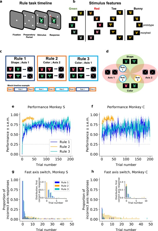
Task design and performance (including all trials).
(a) Schematic of a trial. (b) Stimuli were drawn from a two-dimensional feature space, morphing both color (left) and shape (right). Stimulus categories are indicated by vertical lines and labels. (c) The stimulus–response mapping for the three rules, and an example of a block timeline. (d) Venn diagram showing the overlap between rules. Average performance (sample mean and standard error of the mean) for each rule, for (e) Monkey S and (f) Monkey C. Proportion of responses on the incorrect axis for the first 50 trials of each block for (g) Monkey S and (h) Monkey C. Insets: Trial number of the first response on the correct axis after a block switch, respectively, for Monkeys S and C.

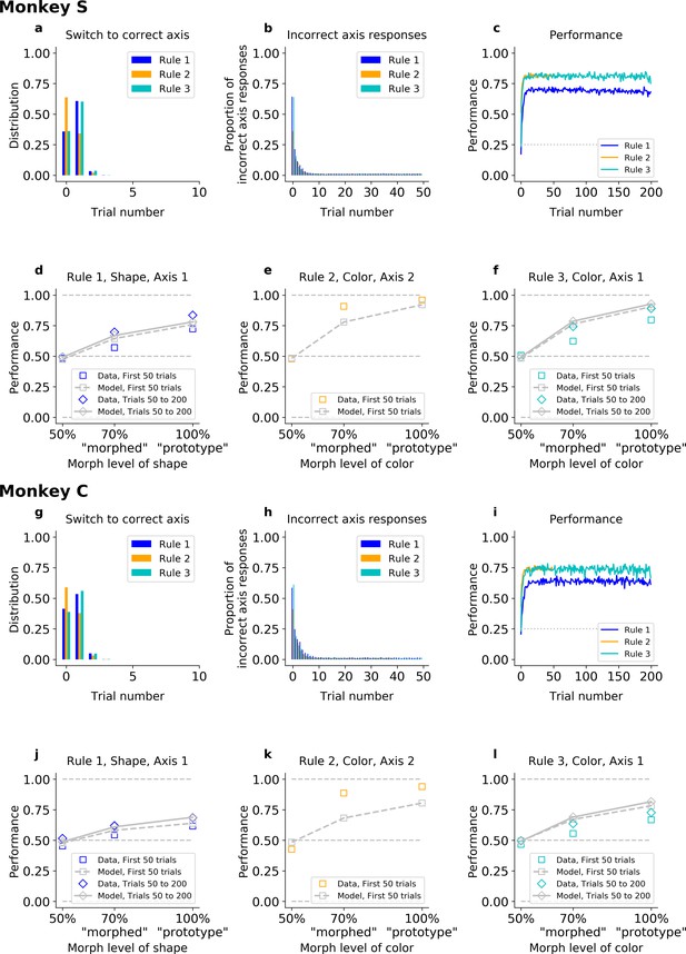
Incremental learner (QL) model fitted on Monkey S behavior (see Figure 2—figure supplement 2 for Monkey C).
(a) Trial number of the first response of the model on the correct axis after a block switch (compare to Figure 1g, inset). (b) Proportion of responses of the model on the incorrect axis for the first 50 trials of each block (compare to Figure 1g). (c) Model performance for each rule (averaged over blocks, compare to Figure 1e).

Incremental learner (QL) model fitted on Monkey C behavior (see Figure 2 for Monkey S).
(a) Trial number of the first response of the model on the correct axis after a block switch (compare to Figure 1h, inset). (b) Proportion of responses of the model on the incorrect axis for the first 50 trials of each block (compare to Figure 1h). (c) Model performance for each rule (averaged over blocks, compare to Figure 1f). Statistics of QL model fitted on Monkey C: First, the model made a response on the correct axis on the first trial with a probability of only 50% in Rules 1, 2, and 3. The model performed 28% of off-axis responses after 20 trials in Rule 1, and 25% in Rules 2 and 3. Second, the model performed correctly on the first trial in only 25% of Rule 2 blocks, and reached only 51% after 20 trials. As a result, on the first 20 trials, the difference in average percent performance was only Δ = 3.3 between Rules 2 and 1, and only Δ = −0.39 between Rules 2 and 3.
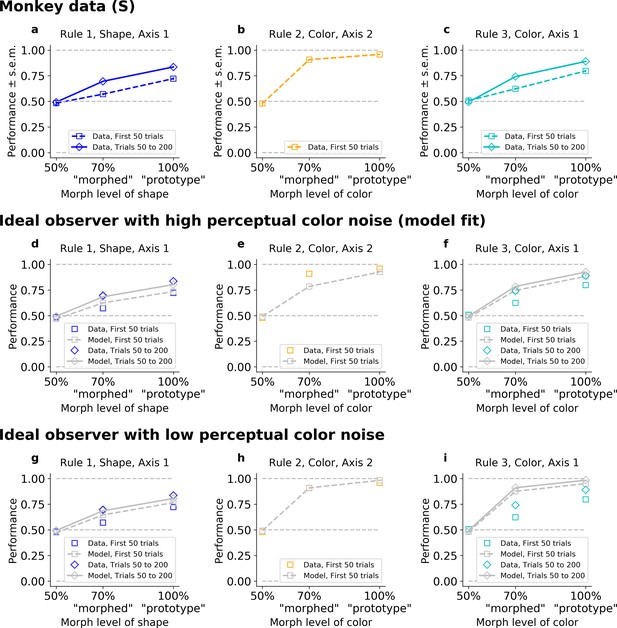
The ideal observer (IO), slow or fast, but not both.
Fitted on Monkey S behavior (see Figure 3—figure supplement 1 for Monkey C). Note that data were collapsed across 50%/150%; 30%/70%/130%/170%; and 0%/100% (non-collapsed psychometric functions can be seen in Figure 5). (a–c) Performance for Rules 1, 2, and 3, as a function of the morphed version of the relevant feature. (d–f) Performance for Rules 1, 2, and 3, for IO model with high color noise. This parameter regime corresponds to the case where the model is fitted to the monkey’s behavior (see Methods). (g–i) Performance for Rules 1, 2, and 3, for IO model with low color noise. Here, we fixed κC = 6.
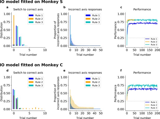
Ideal observer (IO) model fitted on Monkeys S and C.
(a–c) IO model fitted on Monkey S behavior. (a) Trial number of the first response of the model on the correct axis after a block switch (compare to Figure 1e, inset). (b) Proportion of responses of the model on the incorrect axis for the first 50 trials of each block (compare to Figure 1e). (c) Model performance for each rule (averaged over blocks, compare to Figure 1g). (d–f) Same, but for Monkey C. Statistics of IO model fitted on Monkey C: The model responded on the correct axis on the first trial with a probability of 63% in Rule 1, 38% in Rule 2, and 60% in Rule 3. The model maintained the correct axis with very few off-axis responses throughout the block (after trial 20, 1.3% in Rule 1; 6.8%, in Rule 2; 1.3% in Rule 3, Fisher’s test against monkey behavior: p > 0.5 in all rules).
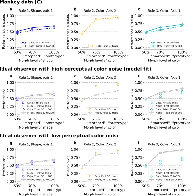
The ideal observer (IO), slow or fast, but not both.
Fitted on Monkey C behavior (see Figure 3 for Monkey S). (a–c) Performance for Rules 1, 2, and 3, as a function of the morphed version of the relevant feature. (d–f) Performance for Rules 1, 2, and 3, for IO model with high color noise. This parameter regime corresponds to the case where the model is fitted to the monkey’s behavior (see Methods). (g–i) Performance for Rules 1, 2, and 3, for IO model with low color noise. Here, we fixed κC = 6. Statistics on Monkey C: There was a discrepancy between the performance of ‘morphed’ stimuli in Rule 2 versus Rule 3, with a difference in average percent performances of Δ = 33 for the first 50 trials in both rules (p < 10−4), and still Δ = 24 if we considered Rule 2 against the last trials of Rule 3 (p < 10−4). The same discrepancy was observed between the performance of ‘prototype’ stimuli in Rule 2 versus Rule 3, with a difference in average percent performances of Δ = 27 for the first 50 trials in both rules (p < 10−4), and still Δ = 21 if we considered the last trials of Rule 3 (p < 10−4). Statistics of IO model fitted on Monkey C: While the IO model, using best-fit parameters, reproduced poor asymptotic performance in Rule 3 by increasing color noise (low concentration), it then failed to capture the high performance on Rule 2 early on. The resulting difference in performance for ‘morphed’ stimuli was only Δ = 4.8 for the first 50 trials and Δ = −7.2 if we considered the last trials of Rule 3 (respectively, Δ = 5.1 and Δ = −8.6 for ‘prototype’).
The ideal observer model including a correct generative prior on the transition between axes given by the specific task structure.
This is defined by fixing the values of the initial belief states over rules to (b1 = 0; b2 = 1; b3 = 0) for a Rule 2 block, and (b1 = 0.5; b2 = 0; b3 = 0.5) for a Rule 1 or 3 block. The model is fitted on Monkeys S and C. (a,b,c,g,h,i) are similar to Figure 2a,b,c. (d,e,f,j,k,l) are similar to Figure 3d,e,f.
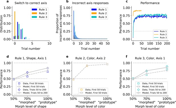
The hybrid learner (HQL) accounts both for fast switching to the correct axis, and slow relearning of Rules 1 and 3.
Model fit on Monkey S, see Figure 4—figure supplement 1 for Monkey C. (a) Trial number for the first response on the correct axis after a block switch, for the model (compare to Figure 1e inset). (b) Proportion of responses on the incorrect axis for the first 50 trials of each block, for the model (compare to Figure 1e). (c) Performance of the model for the three rules (compare to Figure 1g). (d–f) Performance for Rules 1, 2, and 3, as a function of the morphed version of the relevant feature.
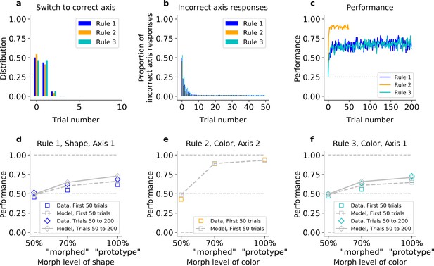
The hybrid learner (HQL) accounts both for fast switching to the correct axis, and slow relearning of Rules 1 and 3.
Model fit on Monkey C, see Figure 4 for Monkey S. (a) Trial number for the first response on the correct axis after a block switch, for the model (compare to Figure 1f inset). (b) Proportion of responses on the incorrect axis for the first 50 trials of each block, for the model (compare to Figure 1f). (c) Performance of the model for the three rules (compare to Figure 1h). (d–f) Performance for Rules 1, 2, and 3, as a function of the morphed version of the relevant feature. Statistics of HQL model fitted on Monkey C: First, the model responded on the correct axis on the first trial with a probability of 50% in Rule 1, 54% in Rule 2, and 47% in Rule 3. The model maintained the correct axis with very few off-axis responses throughout the block (after trial 20, 1.5% in Rule 1; 1.7%, in Rule 2; 1.5% in Rule 3, Fisher’s test against monkey’s behavior: p > 0.5 in all rules). Second, the HQL model could capture the animal’s fast performance on Rule 2 and slower performance on Rules 1 and 3: the difference in average percent performances on the first 20 trials was Δ = 28 both between Rules 2 and 1 and between Rules 2 and 3. Third, not only the HQL model captured the performance ordering on morphed and prototype stimuli for each rule separately, but the model was able to trade-off between initial and asymptotic behavioral performance in Rules 2 and 3, for both ‘morphed’ and ‘prototype’ stimuli. The resulting difference in performance for ‘morphed’ stimuli was Δ = 29 for the first 50 trials and Δ = 24 if we considered the last trials of Rule 3 (respectively, Δ = 29 and Δ = 22 for ‘prototype’).
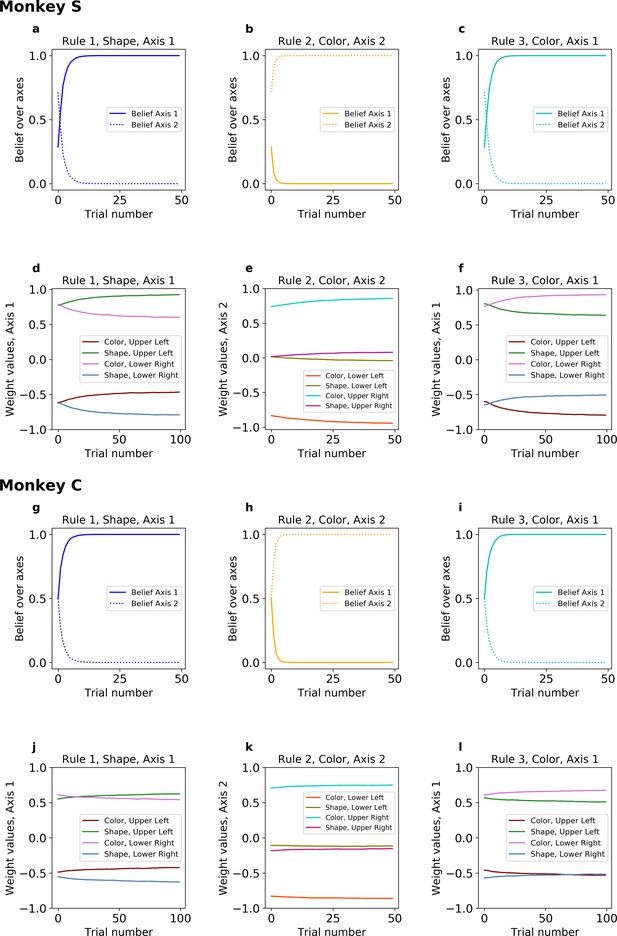
The hybrid learner, beliefs, and weights.
(a–c) Belief over axes when the model is fitted on Monkey S. (d–f) Feature weights values when the model is fitted on Monkey S. (g–i) Belief over axes when the model is fitted on Monkey C. (j–l) Feature weights values when the model is fitted on Monkey C.
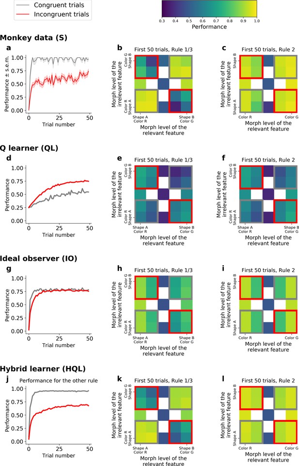
Comparison of incongruency effects in Monkey S and behavioral models (QL, IO, and HQL models).
(a) Performance as a function of trial number for Rules 1 and 3 (combined), for congruent and incongruent trials. (b) Performance for Rules 1 and 3 (combined, first 50 trials), as a function of the morph level for both color (relevant) and shape (irrelevant) features. Gray boxes highlight congruent stimuli, red boxes highlight incongruent stimuli. (c) Performance for Rule 2, as a function of the morph level for both color (relevant) and shape (irrelevant) features. Note the lack of an incongruency effect. (d–f) Same as a–c but for the QL model. (g–i) Same as a–c for the IO model. (j–l) Same as a–c but for the HQL model.
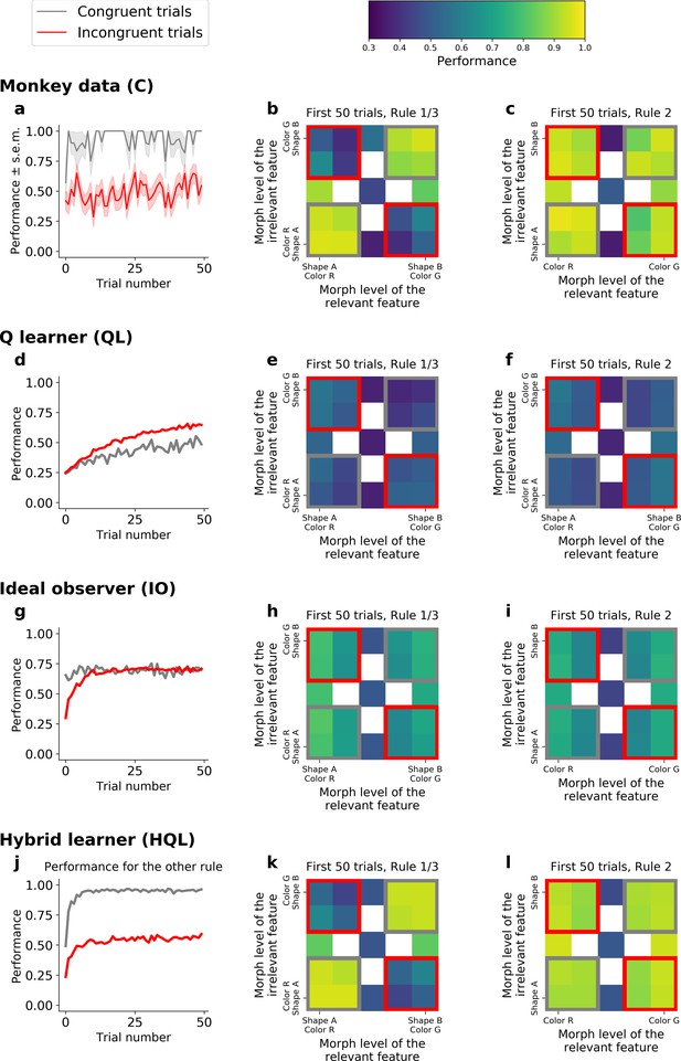
Comparison of incongruency effects in Monkey C and behavioral models (QL, IO, and HQL models).
(a) Performance as a function of trial number for Rules 1 and 3 (combined), for congruent and incongruent trials. (b) Performance for Rules 1 and 3 (combined, first 50 trials), as a function of the morph level for both color (relevant) and shape (irrelevant) features. Gray boxes highlight congruent stimuli, red boxes highlight incongruent stimuli. (c) Performance for Rule 2, as a function of the morph level for both color (relevant) and shape (irrelevant) features. Note the lack of an incongruency effect. (d–f) Same as a–c but for the QL model. (g–i) Same as a–c for the IO model. (j–l) Same as a–c but for the HQL model. Statistics on Monkey C: During early trials of Rules 1 and 3, the monkeys’ performance was significantly higher for congruent trials than for incongruent trials (gray vs. red squares; 93%, confidence interval, CI = [0.91,0.95] vs. 49%, CI = [0.47,0.51], respectively; with Δ = 44; Fisher’s test p < 10−4). There was no difference in performance between congruent and incongruent stimuli during Rule 2 (gray vs. red squares; performance was 94%, CI = [0.91,0.95], and 91%, CI = [0.89,0.92], respectively; with Δ = 2.7; Fisher’s test p = 0.07). Statistics of QL model fitted on Monkey C: The model performed worse on congruent than incongruent trials in Rules 1 and 3 (41% and 52%, respectively; Δ = −10; Fisher’s test p < 10−4), against our behavioral observations. Furthermore, the model produced a difference in performance during Rule 2 (48% for congruent vs. 54% for incongruent; Δ = −6.1; Fisher’s test p < 10−4). Statistics of IO model fitted on Monkey C: Learning quickly reached a low asymptotic performance in Rules 1 and 3, for both congruent and incongruent trials (69% and 67% respectively; Δ = 2.5 only). Statistics of HQL model fitted on Monkey C: The model reproduced the greater performance on congruent than incongruent stimuli in Rules 1 and 3 (94% and 53%, respectively; Δ = 41). It also captured the absence of incongruency effect in Rule 2 (green vs. red squares; 91% and 91%, respectively; Δ = 0.081).
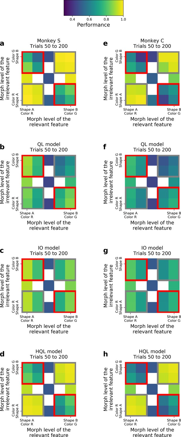
Incongruency effect.
For Monkey S (a), Monkey C (e), and models (respectively, fitted on Monkey S: b–d; and on Monkey C: f–h), for trials 50–200. Each plot represents the performance for Rules 1 and 3 (combined), as a function of morphs for both relevant and irrelevant features. Gray corners for congruent stimuli, red corners for incongruent stimuli.
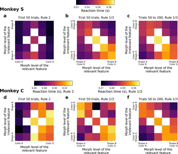
Reaction times.
For Rule 2 blocks (a,d), the first 50 trials of Rule 1/3 blocks (b,e), and the trials 50–200 of Rule 1/3 blocks (c,f) as a function of the relevant and irrelevant features of the morphed stimulus presented. Top row: Monkey S, bottom row: Monkey C. Statistics on Monkey C: Δ (ms) = 14 between incongruent and congruent, t-test p < 10−4.
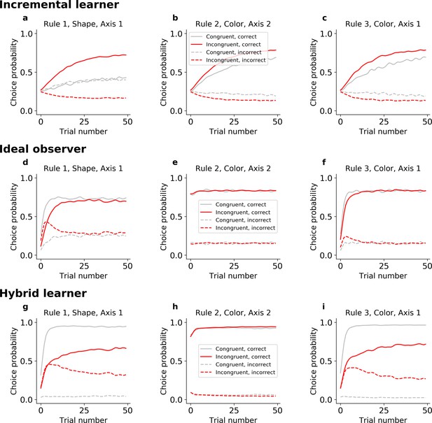
Choice probabilities for the three models fitted on Monkey S.
(a,d,g) Rule 1; (b,e,h) Rule 2; (c,f,i) Rule 3.
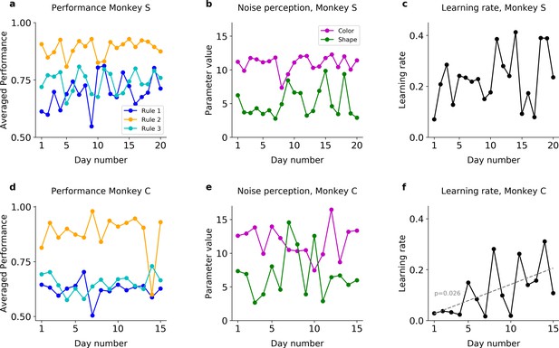
Behavior across days.
(a) Averaged performance over the first 200 trials for Rules 1 and 3, and the first 50 trials for Rule 2, for Monkey S. (b) Noise perception parameter, for color and shape, from the HQL model fit, for Monkey S. (c) Learning rate from the HQL model fit, for Monkey S. (d–f) Same as (a–c) but for Monkey C. Overall, we found no significant trends in the behavior and model parameters across days, with the exception of the learning rate in Monkey C which was moderately significant (not surviving multiple comparison correction).
Tables
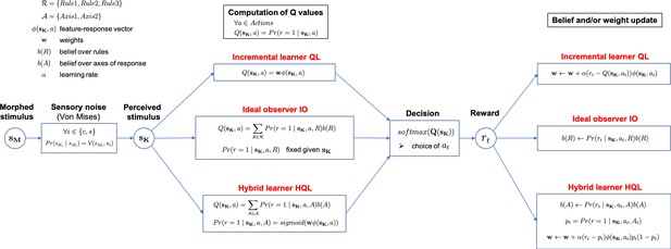
Models parameters.
| Monkey S | Noise perception | Learning rate | Initial belief R1 | Initial belief R3 | Initial belief Axis 1 | Weight decay | Initial weights | |
|---|---|---|---|---|---|---|---|---|
| κ (color) | κ (shape) | α | b1 | b3 | bax | η | w0 | |
| QL model | Mean = 2.2 std = 0.44 | Mean = 1.3 std = 0.27 | Mean = 0.23 std = 0.039 | |||||
| IO model | Mean = 2.4 std = 0.46 | Mean = 1.3 std = 0.31 | Mean = 0.091 std = 0.089 | Mean = 0.14 std = 0.10 | ||||
| HQL model | Mean = 11 std = 1.2 | Mean = 5.1 std = 2.2 | Mean = 0.23 std = 0.10 | Mean = 0.29 std = 0.076 | Mean = 0.046 std = 0.022 | Mean = [−0.61,0.79,0.77,−0.64, −0.83,0.035,0.74,0.040] std = [0.23,0.089,0.13,0.17, 0.053,0.59,0.19,0.57] | ||
| Monkey C | Noise perception | Learning rate | Initial belief R1 | Initial belief R3 | Initial belief Axis 1 | Weight decay | Initial weights | |
| κ (color) | κ (shape) | α | b1 | b3 | bax | η | w0 | |
| QL model | Mean = 1.2 std = 0.13 | Mean = 0.71 std = 0.090 | Mean = 0.18 std = 0.010 | |||||
| IO model | Mean = 1.3 std = 0.21 | Mean = 0.71 std = 0.18 | Mean = 0.35 std = 0.16 | Mean = 0.32 std = 0.16 | ||||
| HQL model | Mean = 12 std = 2.4 | Mean = 7.0 std = 3.4 | Mean = 0.12 std = 0.10 | Fixed to 0.5 | Mean = 0.067 std = 0.060 | Mean = [−0.45,0.56,0.60,−0.56, −0.83,−0.12,0.70,−0.19] std = [0.16,0.12,0.093,0.16, 0.051,0.45,0.25,0.41] | ||


