THINGS-data, a multimodal collection of large-scale datasets for investigating object representations in human brain and behavior
Figures
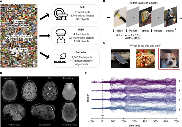
Overview over datasets.
(A) THINGS-data comprises MEG, fMRI and behavioral responses to large samples of object images taken from the THINGS database. (B) In the fMRI and MEG experiment, participants viewed object images while performing an oddball detection task (synthetic image). (C) The behavioral dataset comprises human similarity judgements from an odd-one-out task where participants chose the most dissimilar object amongst three options. (D) The fMRI dataset contains extensive additional imaging data. (E) The MEG dataset provides high temporal resolution of neural response measurements in 272 channels. The butterfly plot shows the mean stimulus-locked response in each channel for four example sessions in one of the participants.
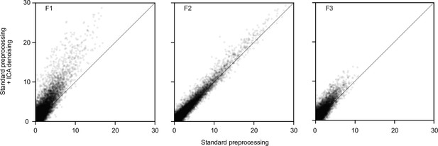
Effects of ICA denoising on fMRI noise ceiling estimates, for all three fMRI participants.
Each data point represents a voxel in a visual mask determined based on the localizer experiment. The x-axis shows the test data noise ceiling in % explainable variance after standard preprocessing. The y-axis shows the respective noise ceiling when the data is additionally denoised with the ICA noise components. All voxels falling above the diagonal show an improved noise ceiling due to ICA denoising.
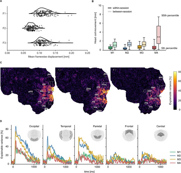
Quality metrics for fMRI and MEG datasets.
fMRI participants are labeled F1-F3 and MEG participants M1-M4 respectively. (A) Head motion in the fMRI experiment as measured by the mean framewise displacement in each functional run of each participant. (B) Median change in average MEG head coil position as a function of the Euclidean distance of all pairwise comparisons between all runs. Results are reported separately for comparisons within sessions and between sessions (see Figure 2—figure supplement 4 for all pairwise distances). (C) fMRI voxel-wise noise ceilings in the test dataset as an estimate of explainable variance visualized on the flattened cortical surface. The labeled outlines show early visual (V1–V3) and category-selective brain regions identified based on the population receptive field mapping and localizer data, respectively. (D) MEG time-resolved noise ceilings similarly show high reliability, especially for occipital, parietal, and temporal sensors.
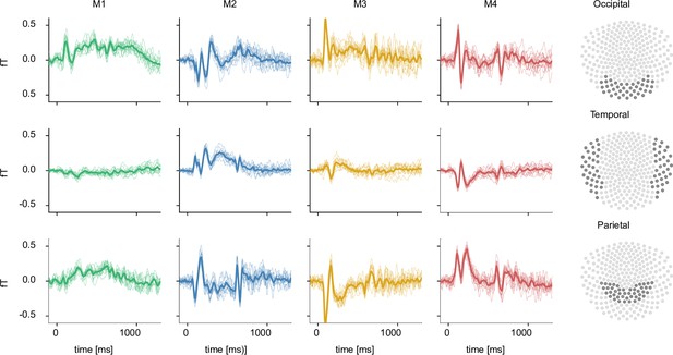
Event-related fields for occipital, temporal, and parietal sensors.
After preprocessing, event-related fields were calculated for each participant (columns 1–4). Every row shows a different sensor group, as depicted in column 5. Thin lines correspond to the average response to the 200 test images per session, while the thick line corresponds to the average across sessions. The high consistency in the evoked signal highlights the comparability of the data between sessions.
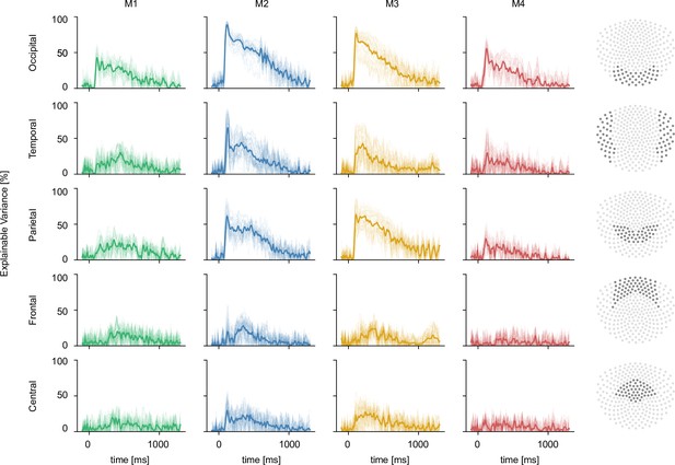
MEG noise ceilings for all sensors.
Every column shows the noise ceiling for a given participant. The last column highlights which sensors were considered for each sensor group (row). Noise ceilings were calculated for each sensor (thin lines) and averaged across sensors in a given sensor group (thick line).
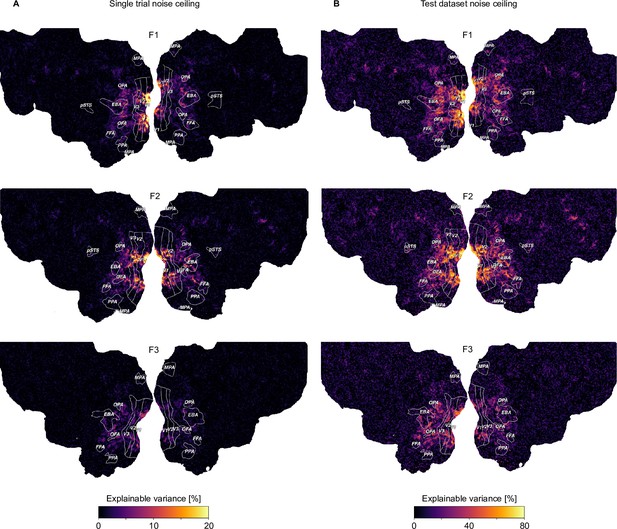
fMRI voxel-wise noise ceilings per participant projected onto the flattened cortical surface.
(A) The noise ceiling estimate on the level of single trial responses. (B) Noise ceiling estimate in the test dataset where responses from 12 trial repetitions can be averaged. Note that the range of noise ceiling values represented by the color map is higher for the test dataset (0–80%) compared to the single trial responses (0–20%).
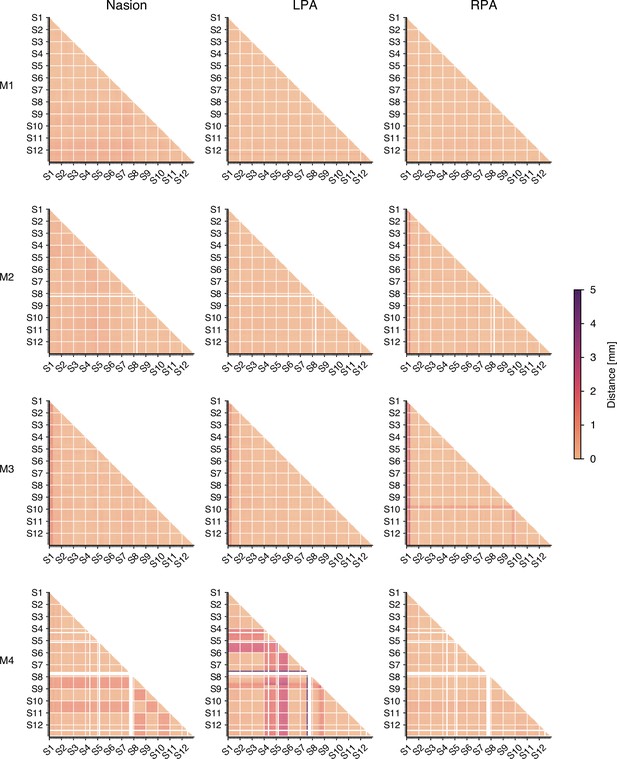
Head coil positioning across runs in the MEG experiment.
Head position was recorded with three marker coils attached at the nasion, left preauricular, and right preauricular. The coil positions were recorded before and after each run. To calculate the distance between runs and sessions, we took the mean of pre- and post-run measurements and calculated the Euclidean distance between all pairs of run measurements. Runs with failed localization were excluded. Overall, head coil positioning was consistent across sessions and runs. However, for participant M4 there were two sessions (S4 and S5) where the left marker coil may not have been attached at the same location as in other sessions, evidenced by low within-session and high between-session distances. Additionally, there may have been a failed measurement in session 8, characterized by large distances to all other measurements. While this indicates that head motion estimates we provided in the main text are rather conservative, researchers should be careful when using the head coil localization from these runs (e.g. for source reconstruction).
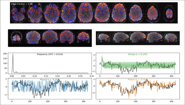
Example visualization used for the manual labeling of independent components.
For the ICA-based denoising, two raters manually labeled a subset of all independent components as signal or noise based on these visualizations. For the depicted example component, both raters labeled it as a noise component related to head motion. The top two rows show the spatial map (thresholded at 0.9) of the independent component overlayed on the mean functional image of that run. The frequency spectrum (third row left) was presented alongside the high-frequency content. The remaining plots show the expected time course of the experimental design (green), physiological noise (blue), and head motion related noise (orange) alongside the time course of the independent component (black) as well as the correlation between the component’s and these expected time courses.
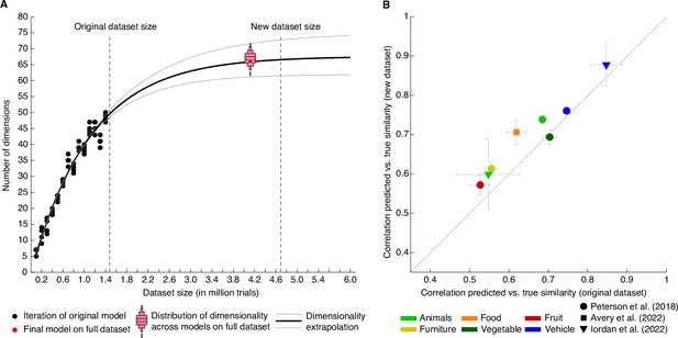
Behavioral similarity dataset.
(A) How much data is required to capture the core representational dimensions underlying human similarity judgments? Based on the original dataset of 1.46 million triplets (Hebart et al., 2020), it was predicted that around 4.5–5 million triplets would be required for the curve to saturate. Indeed, for the full dataset, the dimensionality was found to be 66, in line with the extrapolation. Red bars indicate histograms for dimensionality across several random model initializations, while the final model was chosen to be the most stable among this set. (B) Within-category pairwise similarity ratings were predicted better for diverse datasets using the new, larger dataset of 4.70 million triplets (4.10 million training samples), indicating that this dataset contains more fine-grained similarity information. Error bars reflect standard errors of the mean.
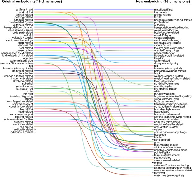
Changes in embedding dimensions between original embedding (49 dimensions) and the new embedding (66 dimensions) based on the full dataset.
Lines correspond to Pearson correlations between old and new dimensions, only showing cases with r>0.3 for dimensions that already have a strong pairing (e.g. ‘artificial/hard’ with ‘metallic/artificial’) and r>0.3 for dimensions without a strong pairing (after correcting for baseline cross-correlation between the original 49 dimensions). These cutoffs were chosen arbitrarily to provide a trade-off between maximizing the information contained in this figure while still effectively visualizing changes in dimensions. 46 out of 49 original dimensions showed strong correlations with new dimensions (all r>0.63), demonstrating that the original embedding was reproduced well. In addition, several dimensions were split up, either revealing more fine-grained distinctions (e.g. ‘sweet/dessert’ rather than ‘food’), disentangling dimensions further (e.g. ‘plant-related/green’ to separate dimensions for ‘plant-related’ and ‘green’), or sometimes remixing them (e.g. ‘tool-related’ and ‘long/thin’ led to ‘pointed/spiky’). Finally, there were a number of dimensions that previously had not been found and also showed no strong relationship to previous dimensions (e.g. ‘fluffy/soft’).
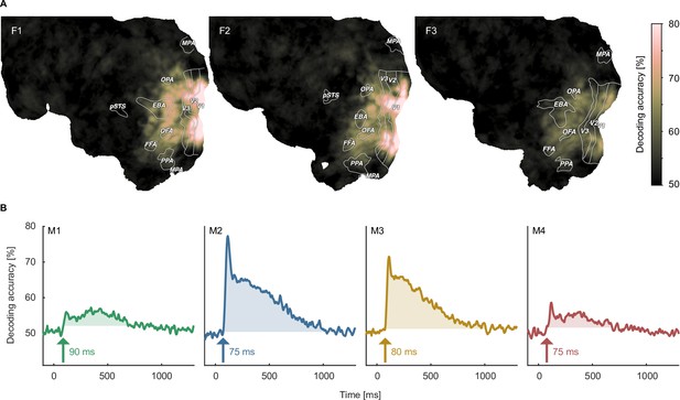
Object image decoding in fMRI and MEG.
(A) Decoding accuracies in the fMRI data from a searchlight-based pairwise classification analysis visualized on the cortical surface. (B) Analogous decoding accuracies in the MEG data plotted over time. The arrow marks the onset of the largest time window where accuracies exceed the threshold which was defined as the maximum decoding accuracy observed during the baseline period.
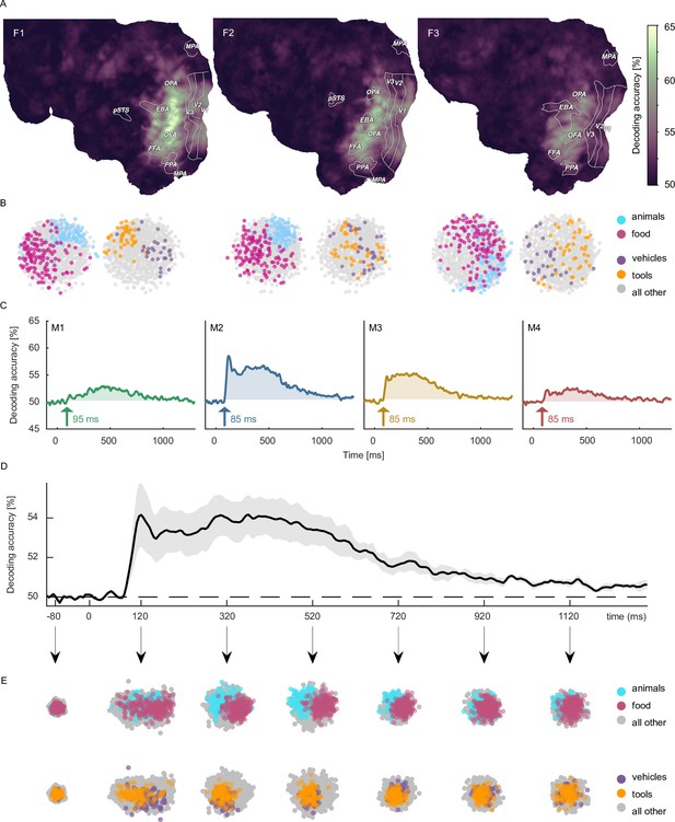
Object category decoding and multidimensional scaling of object categories in fMRI and MEG.
(A) Decoding accuracies in the fMRI data from a searchlight-based pairwise classification analysis visualized on the cortical surface. (B) Multidimensional scaling of fMRI response patterns in occipito-temporal category-selective brain regions for each individual subject. Each data point reflects the average response pattern of a given object category. Colors reflect superordinate categories. (C) Pairwise decoding accuracies of object category resolved over time in MEG for each individual subject. (D) Group average of subject-wise MEG decoding accuracies. Error bars reflect standard error of the mean across participants (n = 4). (E) Multidimensional scaling for the group-level response pattern at different timepoints. Colors reflect superordinate categories and highlight that differential responses can emerge at different stages of processing.
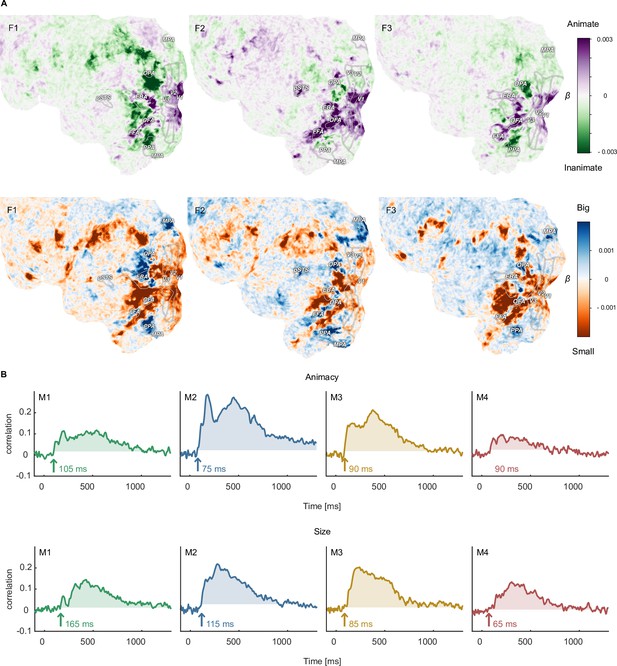
Functional topography and temporal dynamics of object animacy and size.
(A) Voxel-wise regression weights for object animacy and size as predictors of trial-wise fMRI responses. The results replicate the characteristic spoke-like topography of functional tuning to animacy and size in occipitotemporal cortex. (B) Time courses for the animacy (top) and size (bottom) information in the MEG signal. The time courses were obtained from a cross-validated linear regression and show the correlation between the predicted and true animacy and size labels. Shaded areas reflect the largest time window exceeding the maximum correlation during the baseline period.
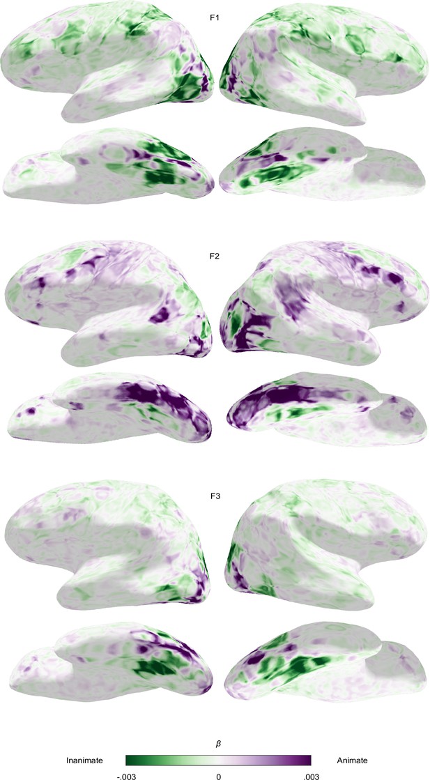
Functional topography of object animacy.
fMRI single trial responses averaged per object concept were predicted with animacy and size ratings obtained from human observers using ordinary least squares linear regression. Voxel-wise regression weights were resampled to an inflated representation of the participant’s individual cortical surface. The animacy regressor was z-scored such that positive weights (purple) indicate a preference for animate objects and negative weights (green) for inanimate objects at a given cortical location. Results are shown for all three participants.
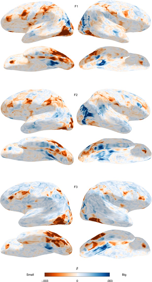
Functional topography of object size.
fMRI single-trial responses averaged per object concept were predicted with animacy and size ratings obtained from human observers using ordinary least squares linear regression. Voxel-wise regression weights were resampled to an inflated representation of the participant’s individual cortical surface reconstruction. The size regressor was z-scored such that positive weights (blue) indicate a preference for big objects and negative weights (orange) for small objects at a given cortical location. Results are shown for all three participants.
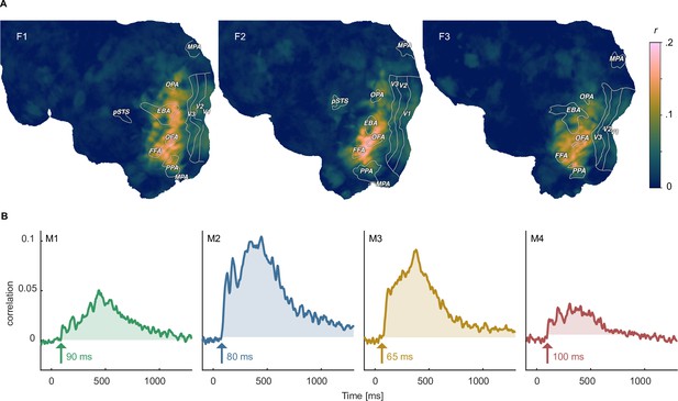
Identifying shared representations between brain and behavior.
(A) Pearson correlation between perceived similarity in behavior and local fMRI activity patterns using searchlight representational similarity analysis. Similarity patterns are confined mostly to higher visual cortex. (B) Pearson correlation between the perceived similarity in behavioral and time-resolved MEG activation patterns across sensors using representational similarity analysis. The largest time window of timepoints exceeding a threshold are shaded. The threshold was defined as the maximum correlation found during the baseline period.
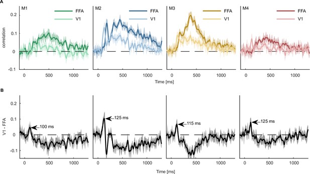
Predicting fMRI regional activity with MEG responses.
(A) Pearson correlation between predicted and true regression labels using mean FFA and V1 responses as dependent and multivariate MEG sensor activation pattern as independent variable. Shaded areas around the mean show bootstrapped confidence intervals (n=10,000) based on a 12-fold cross-validation scheme, leaving one session out for testing in each iteration. The mean across the cross-validation iterations is smoothed over 5 timepoints. (B) Difference between V1 and FFA time-resolved correlations with the peak highlighting when the correlation with V1 is higher than that of FFA. Error bars reflect boostrapped 95% confidence intervals (10,000 iterations).
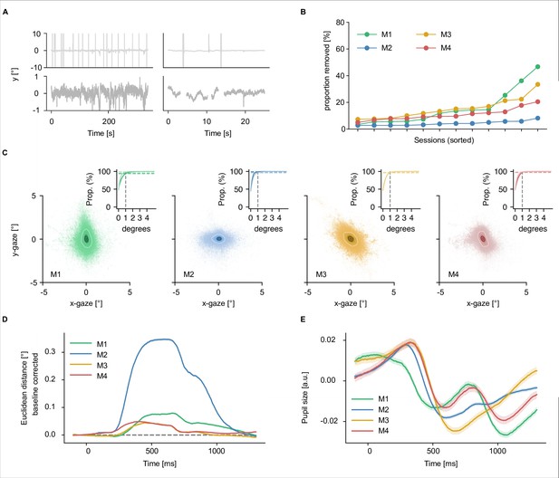
Eye-tracking preprocessing and results.
(A) Visual illustration of the eye-tracking preprocessing routine. Raw data for one example run (top row) and preprocessed data for the same run (bottom row). (B) Amount of eye-tracking data removed during preprocessing in each session for each participant separately, sorted by proportion removed. On average we lost around 10% of the eye-tracking samples during preprocessing. (C) Gaze positions for all four participants. The large panel shows eye positions across sessions for each participant (downsampled to 100 Hz). To quantify fixations, we added rings to the gaze position plots corresponding to containing 25% (black) and 75% (white) of the data. In addition, we examined the proportion of data falling below different thresholds (small panel top right corner within the large panels). The vertical dashed lines indicate the 1 degree mark in all panels. (D) Mean time-resolved distance in gaze position relative to the baseline period in each trial. Shading represents standard error across all trials. (E) Time-resolved pupil size in volts. Larger numbers reflect a larger pupil area. Shading represents standard error across sessions.
Additional files
-
Supplementary file 1
Acquisition parameters for all MRI sequences used in the fMRI dataset.
- https://cdn.elifesciences.org/articles/82580/elife-82580-supp1-v4.docx
-
MDAR checklist
- https://cdn.elifesciences.org/articles/82580/elife-82580-mdarchecklist1-v4.docx


