scRNA-sequencing in chick suggests a probabilistic model for cell fate allocation at the neural plate border
- Centre for Craniofacial and Regenerative Biology, Faculty of Dentistry, Oral and Craniofacial Sciences, King’s College London, United Kingdom
- Bioinformatics and Computational Biology Laboratory, The Francis Crick Institute, United Kingdom
Figures
Figure 1
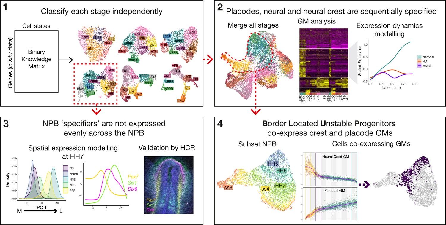
Workflow and summary of findings.
Workflow schematic highlighting key findings from our analysis. Dotted red lines and arrows illustrate data moving from one part of the analysis to the next. The main analysis can be broken into 4 main steps: (1) classify cell states at each developmental stage independently using a binary knowledge matrix; (2) merge cells from all stages to identify global gene modules characterising ectodermal lineage segregation; (3) subset cells at HH7 to model spatial expression patterns across the mediolateral axis; and (4) subset cells at the NPB and identify ‘border located unstable progenitors’ through co-expression of placodal and neural crest gene modules.
Figure 2 with 2 supplements
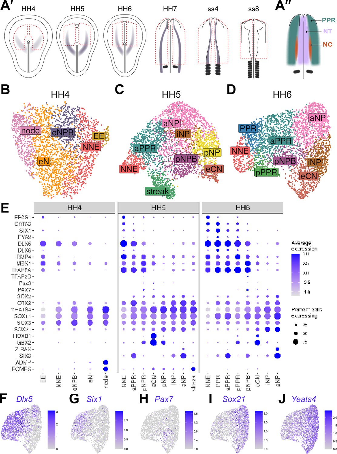
Cells at stages HH4 to HH6 reflect the anterior-posterior and medio-lateral axes in the embryo.
(A’) Dorsal view schematics of chick embryo at stages HH4-ss8 depicting the ectodermal tissue region dissected for 10 x scRNAseq (red dotted line). Purple shading illustrates previously characterized region of Pax7 expression (Basch et al., 2006). (A’’) Schematic of a 1-somite stage (HH7) chick embryo illustrating the pre-placodal region (PPR), neural crest (neural crest) and neural tube (NT). (B–D) UMAP plots for cells collected at HH4-/4 (primitive streak), HH5 (head process), HH6 (head fold) stages. Cell clusters are coloured and labelled based on their semi-unbiased cell state classifications (binary knowledge matrix available in Supplementary file 1). (E) Dot plots displaying the average expression of key marker genes across cell states at HH4, HH5 and HH6. The size of the dots represents the number of cells expressing a given gene within each cell population. (F) Feature plots revealing the mediolateral expression of key marker genes at HH6 and their overlapping expression.
Figure 2—figure supplement 1
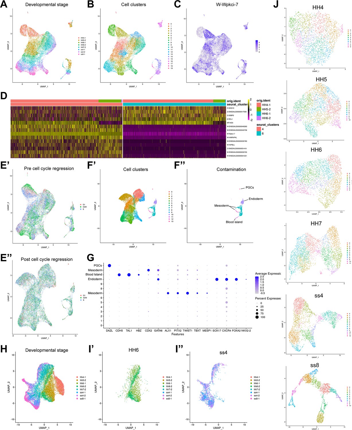
Data analysis and quality control.
(A–B) UMAP of full dataset prior to regressing out confounding factors. Cells are coloured by developmental stage (A) and Seurat cell clusters (B). (C) Feature plot displaying W (male) sex-chromosome gene Wpkci-7, illustrating the cell sex effect after clustering. (D) Heatmap of selected sex genes across clusters 4 and 6. These clusters contain mostly cells from HH4 and highlight the clear sex effect of W and Z chromosome genes between these clusters. (E) UMAP of cells prior to (E’) and post (E’’) regressing out the cell cycle effect. (F’) UMAP displaying cell clusters after regressing out sex and cell cycle effects. (F’’) UMAP highlighting contaminating cell states following cell state classification. These include primordial germ cells (PGCs), mesoderm, endoderm, and blood islands. (G) Dotplot for the expression of genes used for identification of contaminating cell clusters. (H) UMAP of all cells after filtering of contaminating populations and regressing out confounding variables. Cells are coloured by developmental stage. (I) UMAP plots showing successful integration of two sequencing batches at stages HH6 (I’) and ss4 (I’’). (J) UMAPs displaying cell clusters calculated at each developmental timepoint. Individual stages are subset from the full filtered dataset displayed in (H).
Figure 2—figure supplement 2
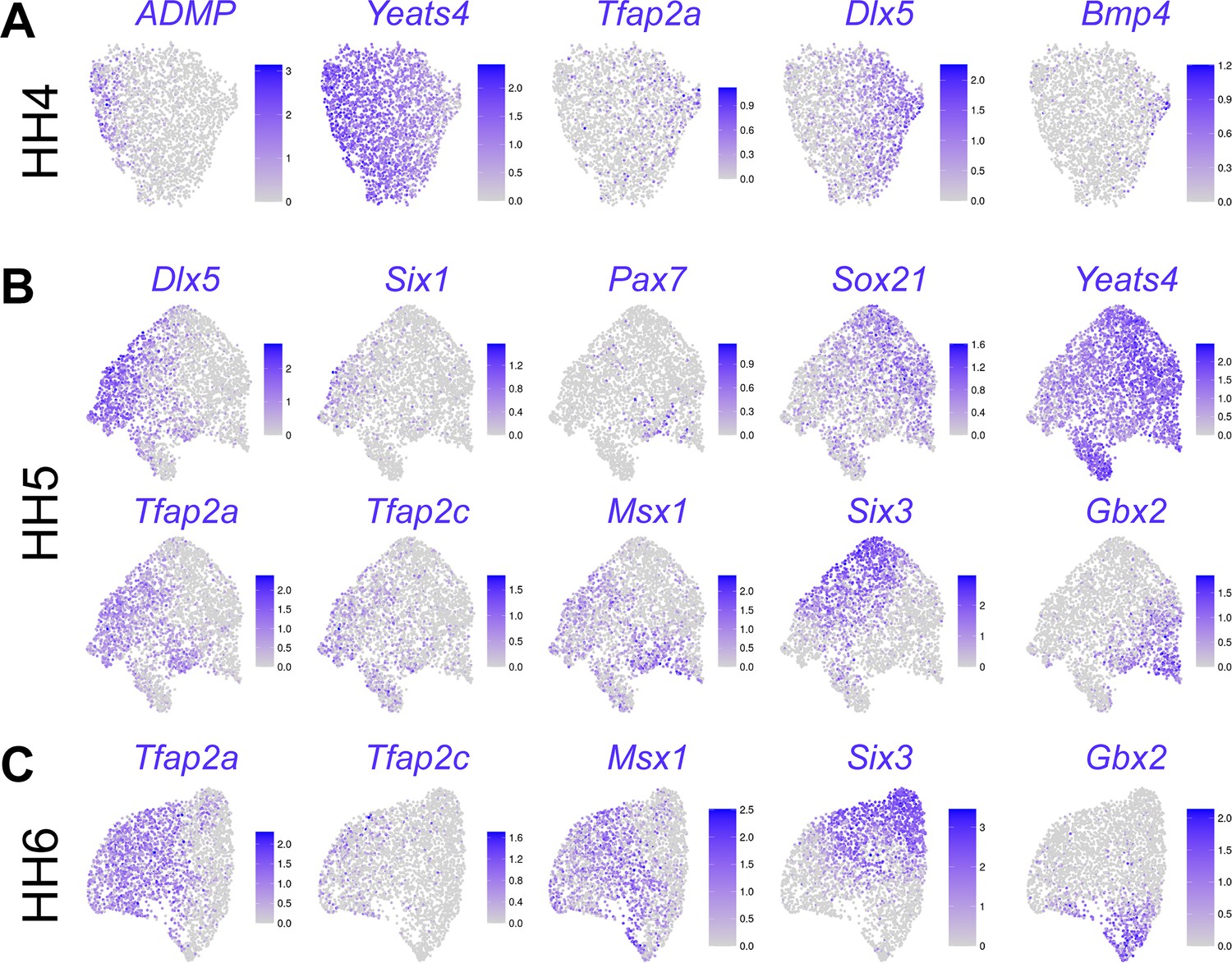
Feature plots showing expression of marker genes on UMAPs of developmental stages HH4 (A), HH5 (B), and HH6 (C).
Figure 3 with 1 supplement
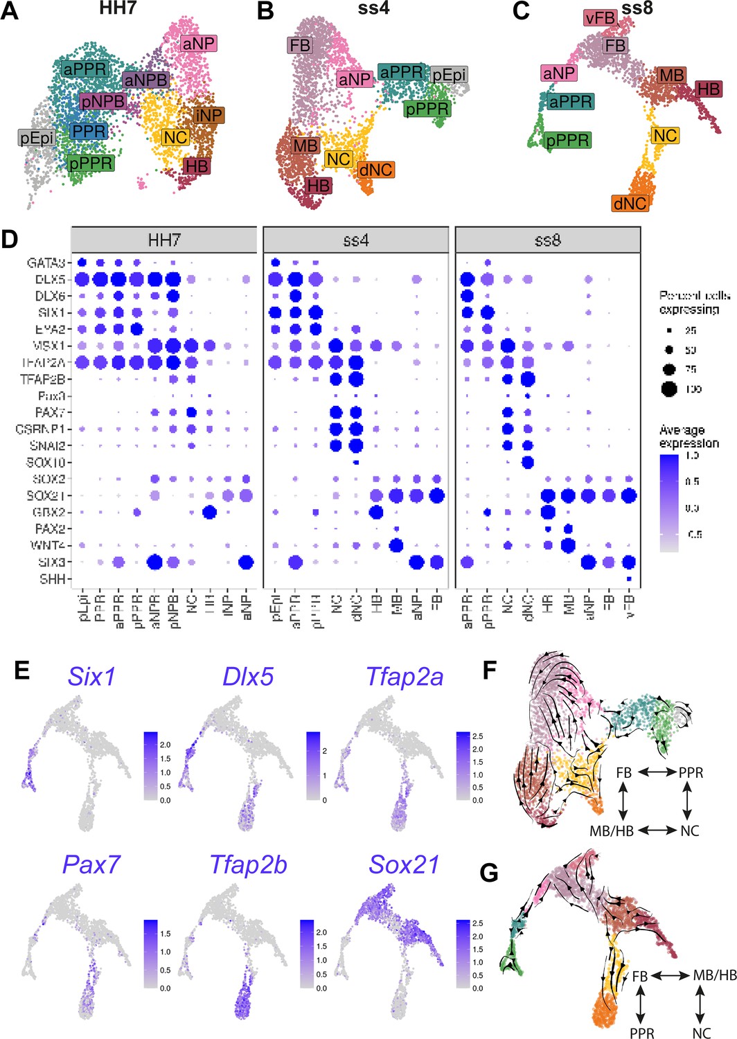
Increased cell diversity and lineage segregation from HH7 to ss8.
(A–C) UMAP plots for cells collected at HH7 (1 somite stage), ss4 (4 somite stage), and ss8 (8 somite stage). Cell clusters are coloured and labelled based on their semi-unbiased cell state classifications (binary knowledge matrix available in Supplementary file 1). (D) Dot plots displaying the average expression of key marker genes across cell states at HH7, ss4, and ss8. The size of the dots represents the number of cells expressing a given gene within each cell population. (E) Feature plots revealing the expression of the pioneer factor Tfap2a and lineage restricted expression of neural (Sox21), placodal (Six1, Dlx5,), and neural crest (Pax7, Tfap2b) markers. (F–G) UMAP plots for ss4 and ss8 overlaid with RNA velocity vectors depicting the predicted directionality of transcriptional change. Cells are coloured by cell state classification (shown in B and C). Schematics summarise the key fate segregation events taking place at these stages predicted by RNA velocity analysis.
Figure 3—figure supplement 1
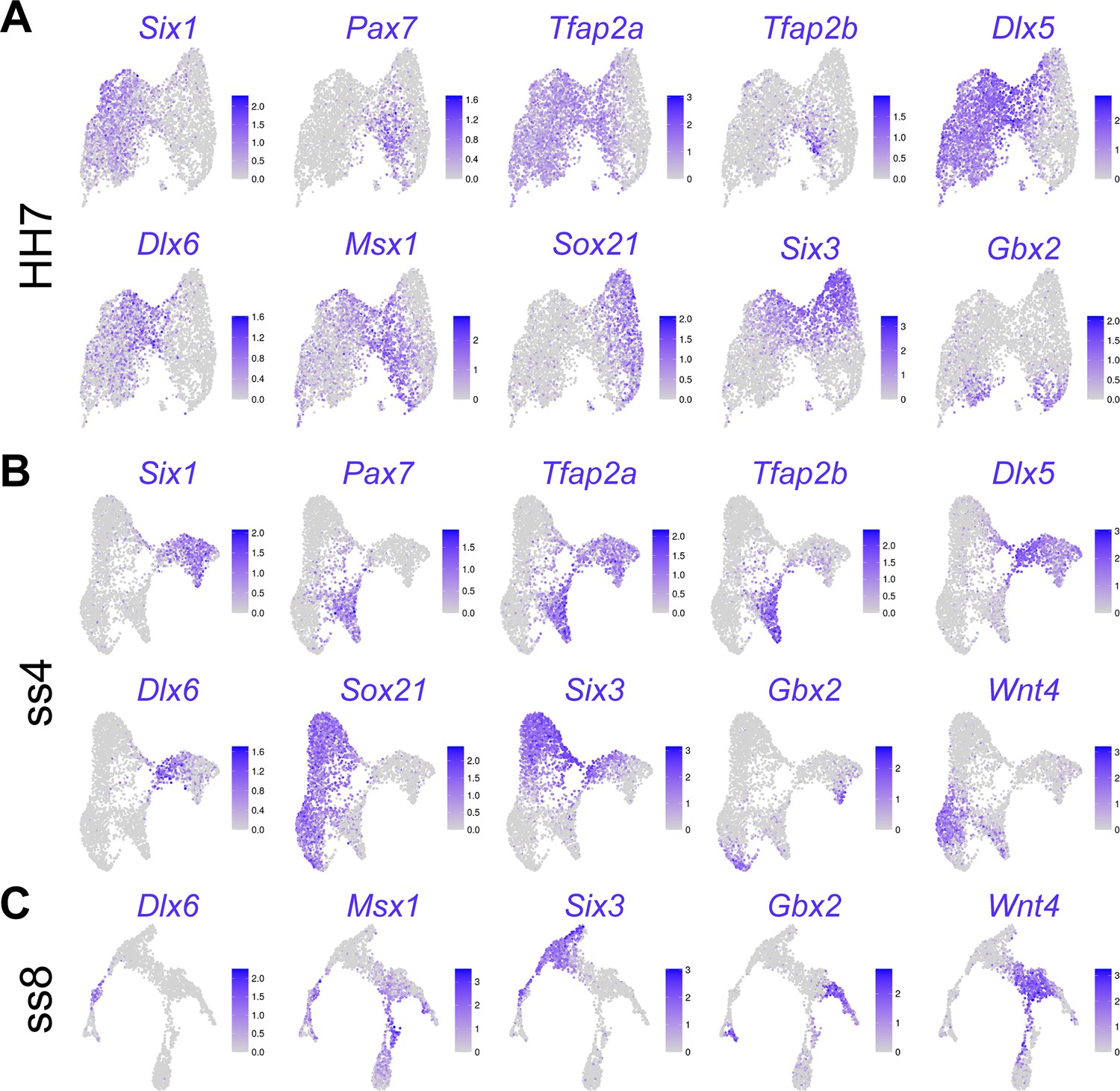
Feature plots showing expression of marker genes on UMAPs of developmental stages HH7 (A), ss4 (B), and ss8 (C).
Figure 4 with 1 supplement
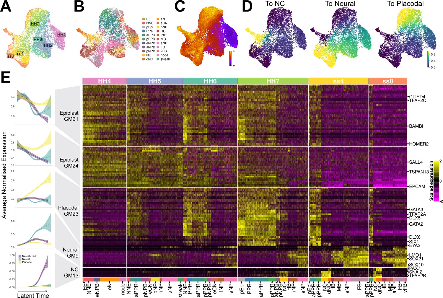
Gene module dynamics reveal key differences between the segregation of the PPR, neural crest and neural fates.
(A) UMAP plot for the full dataset (HH4-ss8 combined) coloured and labelled by stage. (B) UMAP plot for the full dataset coloured by cell state classifications. Cell state classifications were calculated independently for each stage and transferred across for visualisation of the full dataset. (C) UMAP plot of the full dataset (HH4-ss8) showing cell latent time values. (D) UMAP plots of the full dataset showing the fate absorption probabilities of each cell towards one of the three defined terminal states: neural crest, neural and placodal. (E) Left: Gene module dynamics plots displaying generalised additive models (GAMs) of average normalised gene module expression across latent time. GAMs are weighted by the fate absorption probability of each cell towards one of the three terminal states (placodal, neural crest and neural). Shaded area represents upper and lower 95% confidence intervals. Right: Heatmap of gene modules that display fate-specific expression (full list of gene modules available in Figure 4—source data 1). Gene modules were first unbiasedly filtered based on their differential expression between cell states (see methods and Figure 4—figure supplement 1A). Gene modules were further manually filtered based on expression patterns described in the literature (see results section: Defining neural, neural crest, and placodal gene modules). Key genes of interest are highlighted on the right (for full gene list see Figure 4—source data 1).
-
Figure 4—source data 1
Gene lists from gene modules calculated on the full dataset and filtered to include only those differentially expressed between cell states and not sequencing batches, and then further filtered to include only those that are differentially expressed between the neural, neural crest and placodal fates at ss8.
Gene modules (9 in total) are shown in Figure 4—figure supplement 1A.
- https://cdn.elifesciences.org/articles/82717/elife-82717-fig4-data1-v2.txt
Figure 4—figure supplement 1
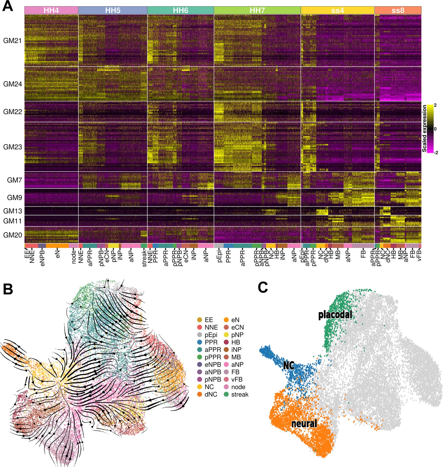
Gene modules and pseudo-time analysis.
(A) Gene modules calculated across the full dataset (full list of gene modules available in Figure 4—source data 1). Gene modules were unbiasedly filtered to include those that only display differential expression between cell states and not between sequencing batches and then further filtered to include only those that are differentially expressed between the neural, neural crest, and placodal cell states at ss8. 9 gene modules remained after filtering. (B) UMAP plot of the full dataset overlaid with RNA velocity vectors depicting the predicted directionality of transcriptional change. Cells coloured by cell state. (C) Selected terminal states (placodal, neural crest and neural) used for CellRank lineage inference.
Figure 5 with 1 supplement
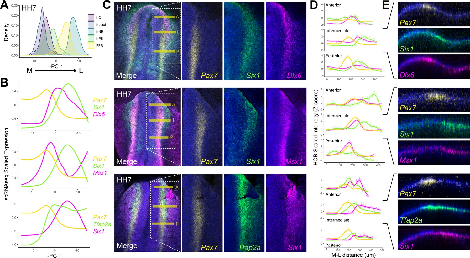
HCR validates spatial restriction of classical NPB specifiers.
(A) Distribution of cells at HH7 from major ectodermal cell lineages across principal component 1 (PC 1), revealing medio-lateral patterning across this axis. The x-axis has been inverted to reflect the positioning of cell populations across the medio-lateral axis in vivo. (B) Spatial gene expression modelling of key placodal and neural crest specifiers at HH7 across the inverse of PC 1. Generalised additive models were fitted for each gene to predict their medio-lateral pattern of expression in the embryo. (C) Whole mount in situ hybridisation chain reaction (HCR) images at HH7 for combinations of markers modelled in B. Overlayed dotted box in the merged image show the region of interest displayed for each separated colour channel. (D) Fluorescent intensity measurements taken at anterior ‘A’, intermediate ‘I’ and posterior ‘P’ regions depicted by the yellow bars in C. Intensity measurements were scaled for each gene across the three axial levels to allow for relative comparisons between different axial regions. (E) Virtual crosssections taken from the intermediate region, highlighting expression of each marker within the embryonic ectoderm. Scale bars in C represent 100 μm (left image) and 50 μm (right image); they apply to all images in the same column. Bar in E represents 100 μm and applied to all sections.
Figure 5—figure supplement 1
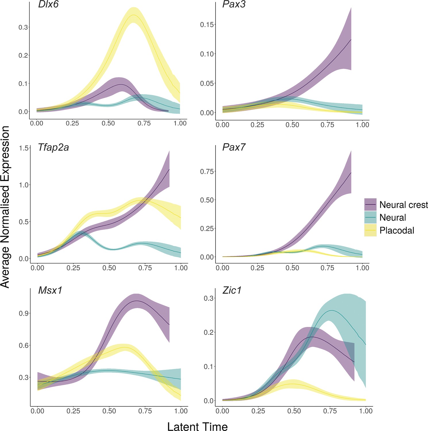
Generalised additive models (GAMs) of average normalised gene expression for previously characterised neural plate border ‘specifiers’.
Gene expression was weighted in the GAM using the placodal fate lineage absorption probability. GAMs highlight that these genes are upregulated within alternate ectodermal cell fates.
Figure 6 with 1 supplement
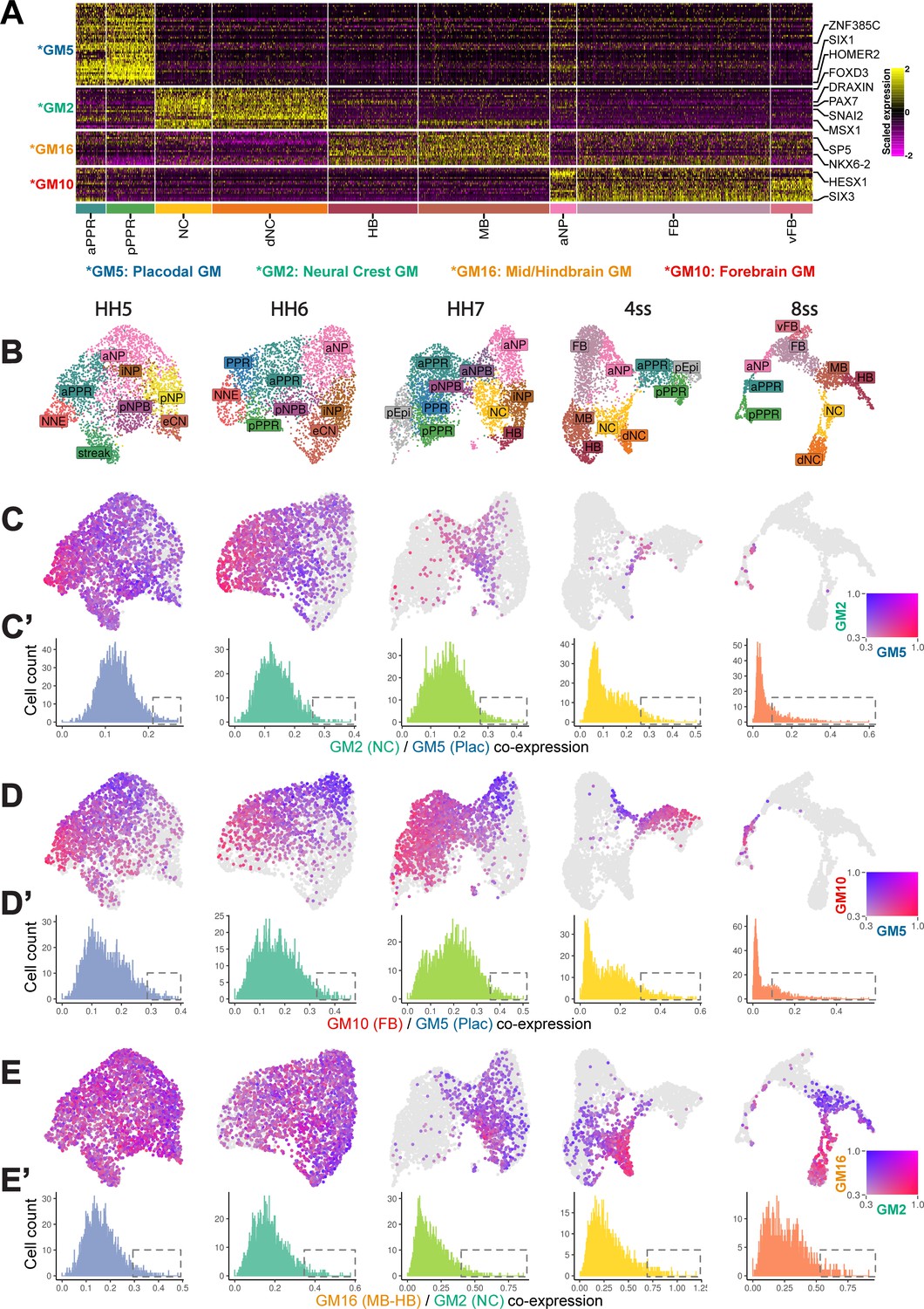
Border-Located Undecided Progenitors’ (BLUPs) co-express placodal and neural crest gene modules.
(A) Heatmap displaying pan-placodal (GM5), pan-neural crest (GM2), mid-hindbrain (GM16), and forebrain (GM10) gene modules at ss8 which have been subset from gene modules in Figure 6—figure supplement 1A. (B) UMAP plots from each developmental stage coloured by cell state. (C) Co-expression analysis of the pan-neural crest and pan-placodal modules (see Materials and methods) at each developmental stage. Cells which co-express both modules above 0.3 are coloured. (C’) Histograms revealing the distribution of co-expression (calculated as the product of gene module expression) of the pan-neural crest and pan-placodal modules at each developmental stage. At later stages (ss4-ss8), the distribution of co-expression shifts from a normal to a negative binomial distribution. Dashed boxes highlight the shift in the proportion of cells maintaining relative high co-expression at later developmental stages. (D) Co-expression analysis of pan-placodal (GM5) and forebrain (GM10) gene modules. Cells which co-express both modules above 0.3 are coloured. (D’) Histograms revealing the distribution of co-expression (calculated as the product of gene module expression) of pan-placodal and forebrain gene modules at each developmental stage. (E) Co-expression analysis of neural crest (GM2) and mid-hindbrain (GM16) gene modules. Cells which co-express both modules above 0.3 are coloured. (E’) Histograms revealing the distribution of co-expression (calculated as the product of gene module expression) of neural crest and mid-hindbrain gene modules at each developmental stage.
-
Figure 6—source data 1
Gene lists from gene modules calculated at ss8 and filtered to include only those differentially expressed between cell states.
Gene modules (15 in total) are shown in Figure 6—figure supplement 1A.
- https://cdn.elifesciences.org/articles/82717/elife-82717-fig6-data1-v2.txt
Figure 6—figure supplement 1
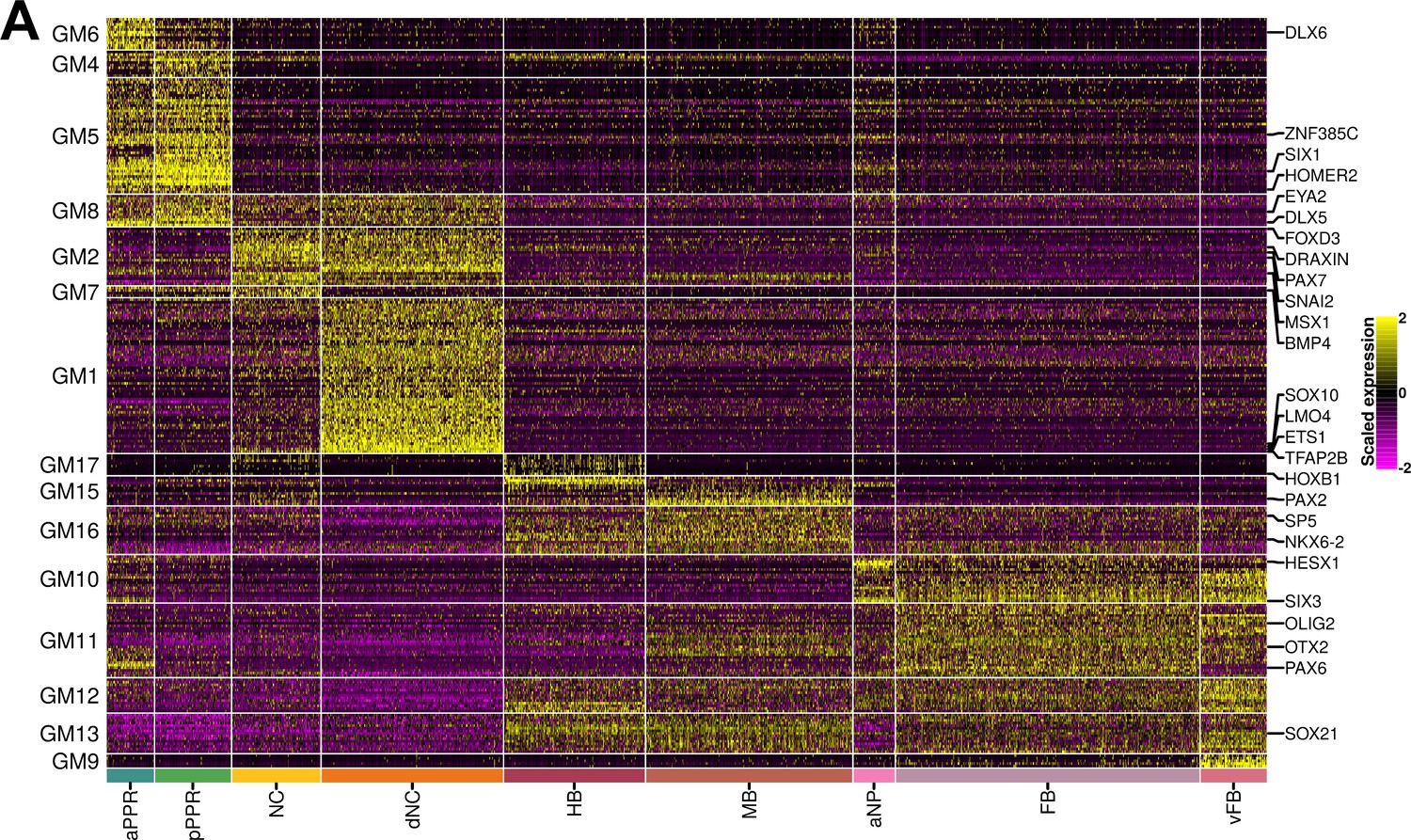
Gene modules calculated from ss8.
(A) Heatmap showing gene modules calculated from ss8 cells and then filtered to include only those that are differentially expressed between cell states (see Materials and methods; full list of gene modules available in Figure 6—source data 1). GM5, GM2, GM16, and GM10 are highlighted as the selected pan-placodal, pan-neural crest, mid-hindbrain and forebrain gene modules respectively used for subsequent co-expression analysis.
Figure 7 with 1 supplement
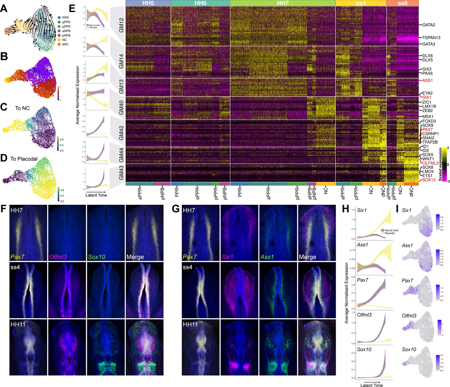
NPB gene module analysis reveals temporal hierarchy of gene expression during development of neural crest and placodes.
(A) UMAP plot with cells coloured by cell state classifications and overlaid with RNA velocity vectors depicting the predicted directionality of transcriptional change. (B) UMAP plot of the NPB subset with cells coloured by latent time. (C–D) UMAP plots showing the fate absorption probabilities of each cell towards the specified terminal states (neural crest or placodes). (E) Left: Gene module dynamics plots displaying generalised additive models (GAMs) of average normalised gene module expression across latent time. GAMs are weighted by the fate absorption probability of each cell towards either placodal or neural crest terminal states. Shaded area represents upper and lower 95% confidence intervals. Right: Heatmap showing gene modules calculated across the NPB subset (full list of gene modules available in Figure 7—source data 1). To identify neural crest and placodal cell state signatures, gene modules were filtered to include those that show differential expression between placodal and neural crest cell states (see methods). Genes specified as neural crest or placodal in our binary knowledge matrix (Supplementary file 1) were selected as bait genes to further filter the gene module list for visualisation. Known and novel placodal and neural crest markers highlighted in red were validated by in situ hybridisation chain reaction (HCR) (F–G). (F) Whole mount in situ HCR at HH7, ss4 and HH11 validating the expression of Olfml3 at the NPB and delaminating neural crest. (G) Whole mount in situ HCR at HH7, ss4 and HH11 validating the expression of Ass1 in the pre-placodal region. (H) Gene dynamics displaying GAMs of average normalised gene expression across latent time. GAMs are weighted by the fate absorption probability of each cell towards either placodal or neural crest lineages. Shaded area represents upper and lower 95% confidence intervals. (I) Feature plots for genes validated by in situ HCR on the HH7 stage UMAP. Scale bars in G represent 100 μm; bars apply to all images in the same row.
-
Figure 7—source data 1
Gene lists from gene modules calculated in the NPB subset and filtered to include only those that show differential expression between cell states and not sequencing batches, and then further filtered to include only those containing genes that were defined within neural crest, neural crest or PPR cell states in the binary knowledge matrix.
Gene modules (7 in total) shown in Figure 7E.
- https://cdn.elifesciences.org/articles/82717/elife-82717-fig7-data1-v2.txt
Figure 7—figure supplement 1
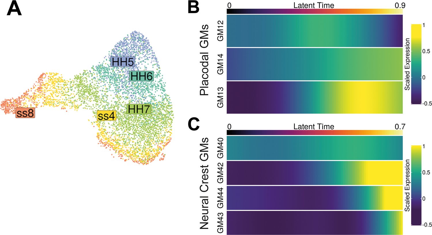
Gene modules from the NPB subset and their expression acorss latent time.
(A) UMAP plot of the neural plate border (NPB) subset coloured by cell state.(B) Heatmap displaying predicted scaled expression of placodal gene modules (GM12, GM13, and GM14) within the placodal lineage across latent time. Gene expression was predicted by fitting a generalised additive model (GAM) which models scaled gene expression as a function of latent time. Gene expression was weighted in the GAM using the placodal fate lineage absorption probability. (C) Heatmap displaying predicted scaled expression of neural crest gene modules (GM40, GM42, GM43, and GM44) within the neural crest lineage across latent time. Gene expression was modelled as in (A) but using neural crest fate absorption probabilities to weight gene expression.
Figure 8
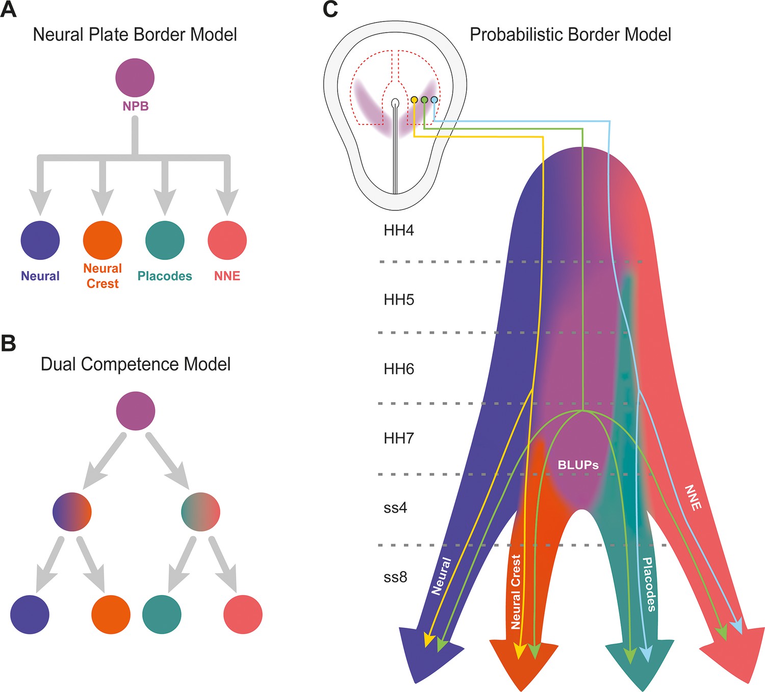
Probabilistic border model resolves conflicting models of lineage segregation at the neural plate border.
(A) Schematic illustrating the neural plate border model. This model illustrates that cells at the neural plate border are multipotent and able to give rise to neural, neural crest, placodal, and non-neural ectoderm (NNE) lineages. (B) Schematic illustrating the dual competence model. This model suggests that the neural plate border is first defined into non-neural/placodal and neural crest/neural competence domains prior to further subdivision into each of the final four cell lineages. (C) Schematic illustrating the probabilistic border model. This model proposes a probabilistic model of cell fate allocation which is intrinsically linked to the spatiotemporal positioning of a cell. We suggest that cells located within the medial neural plate border (yellow cell lineage) will give rise to neural and neural crest, cells within the lateral neural plate border (blue cell lineage) to non-neural ectoderm and placodes, whilst subsets of cells (including Border Located Undecided Progenitors) will remain in an undecided state and continue to give rise to all four lineages even at late stages of neurulation (green cell lineage). Shaded background colours represent the cell state space.
Additional files
-
Supplementary file 1
Binary knowledge matrix used for unbiased cell state classification.
This matrix was established by binarizing the expression of 76 genes across 24 putative cell states based on in situ hybridisation expression patterns obtained from the literature.
- https://cdn.elifesciences.org/articles/82717/elife-82717-supp1-v2.csv
-
MDAR checklist
- https://cdn.elifesciences.org/articles/82717/elife-82717-mdarchecklist1-v2.docx
Download links
A two-part list of links to download the article, or parts of the article, in various formats.
Downloads (link to download the article as PDF)
Open citations (links to open the citations from this article in various online reference manager services)
Cite this article (links to download the citations from this article in formats compatible with various reference manager tools)
scRNA-sequencing in chick suggests a probabilistic model for cell fate allocation at the neural plate border
eLife 12:e82717.
https://doi.org/10.7554/eLife.82717


