Neural population dynamics of computing with synaptic modulations
- Allen Institute, MindScope Program, United States
Figures
Figure 1
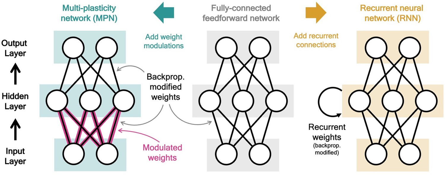
Two neural network computational mechanisms: synaptic modulations and recurrence.
Throughout this figure, neurons are represented as white circles, the black lines between neurons represent regular feedforward weights that are modified during training through gradient descent/backpropagation. From bottom to top are the input, hidden, and output layers, respectively. (Middle) A two-layer, fully connected, feedforward neural network. (Left) Schematic of the MPN. Here, the pink and black lines (between the input and hidden layer) represent weights that are modified by both backpropagation (during training) and the synapse modulation matrix (during an input sequence), see Equation 1. (Right) Schematic of the Vanilla RNN. In addition to regular feedforward weights between layers, the RNN has (fully connected) weights between its hidden layer from one time step to the next, see Equation 3.
Figure 2
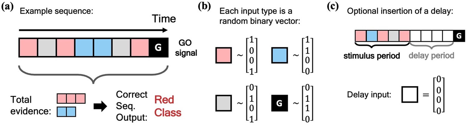
Schematic of simple integration task.
(a) Example sequence of the two-class integration task where each box represents an input. Here and throughout this work, distinct classes are represented by different colors. In this case, red and blue. The red/blue boxes represent evidence for their respective classes, while the grey box represents an input that is evidence for neither class. At the end of the sequence is the ‘go signal’ that lets the network know an output is expected. The correct response for the sequence is the class with the most evidence; in the example shown, the red class. (b) Each possible input is mapped to a (normalized) random binary vector. (c) The integration task can be modified by the insertion of a ‘delay period’ between the stimulus period and the go signal. During the delay period, the network receives no input (other than noise).
Figure 3 with 3 supplements
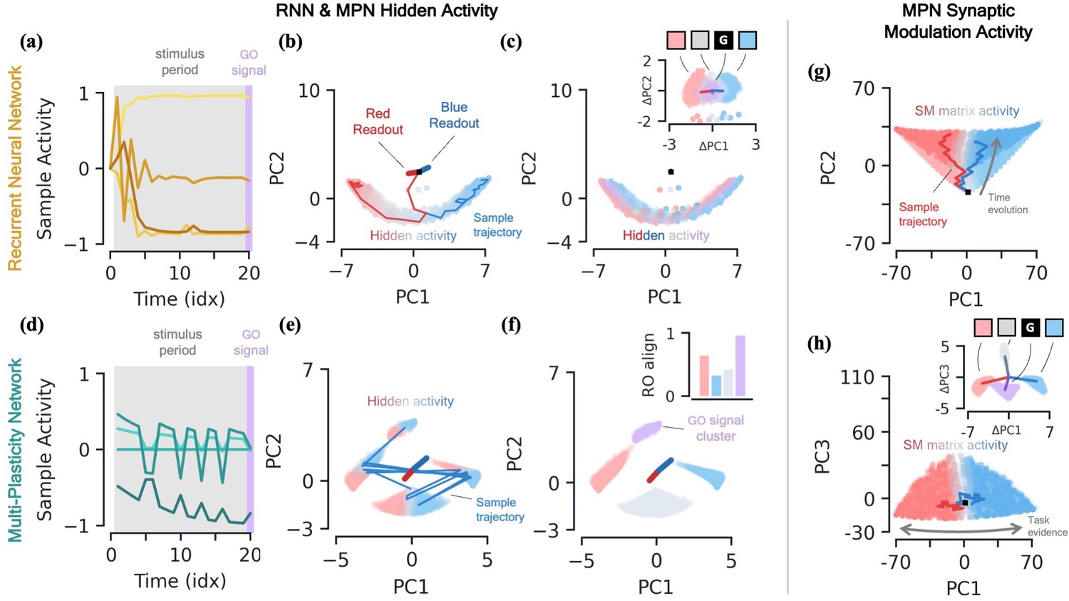
Two-class integration: comparison of multi-plasticity network and RNN dynamics.
(a-c) Vanilla RNN hidden neuron dynamics, see Figure 3—figure supplement 1 for GRU. (a) Hidden layer neural activity, , for four sample neurons of the RNN as a function of sequence time (in units of sequence index). The shaded grey region represents the stimulus period during which information should be integrated across time and the thin purple-shaded region representing the response to the go signal. (b) Hidden neuron activity, collected over 1000 input sequences, projected into their top two PCA components, colored by relative accumulated evidence between red/blue classes at time (Methods 5.5). Also shown are PCA projections of sample trajectories (thin lines, colored by class), the red/blue class readout vector (thick lines), and the initial state (black square). (c) Same as (b), with now colored by input at the present time step, (four possibilities, see inset). The inset shows the PCA projection of as a function of the present input, , with the dark lines showing the average for each of the four inputs. [d-f] MPN hidden neuron dynamics, see Figure 3—figure supplement 1 for MPNpre. (d) Same as (a). (e) Same as (b). (f) Same as (c), except for inset. The inset now shows the alignment of each input-cluster with the readout vectors (Methods 5.5). [g-h] MPN synaptic modulation dynamics. (g) Same as (b), but instead of hidden neuron activity, the PCA projection of the SM matrices, , collected over 1000 input sequences. Final are colored slightly darker for clarity. (h) Same as (g), with a different -axis. The inset is the same as that shown in (b), but for .
Figure 3—figure supplement 1
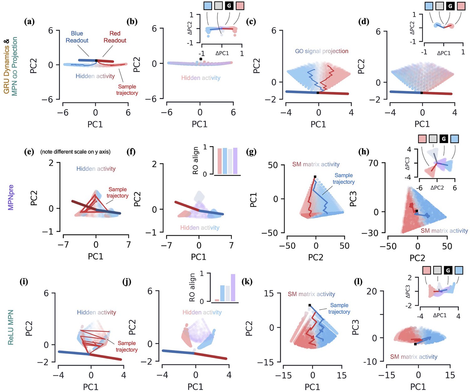
Two-class integration: additional network dynamics.
(a-b) GRU dynamics. (a) GRU hidden activity, projected into their top two PCA components, colored by relative evidence between red/blue classes (Methods). Also shown are PCA projections of sample trajectories (thin lines), the red/blue class readout vector (thick lines), and initial state (black square). (b) Same as (a), colored by input label. The inset shows a scatter of as a function of the current input, , with the dark line showing the average for each input. (c-d) MPN go signal projections. (c) The go signal projection, see Equation 14, of the SM matrix activity shown in Figure 3. The resulting projections are low-dimensional and thus projected onto their top two PC directions. The plot shown colors the projections by accumulated evidence. (d) Same as (c), but the projections are colored by present input. Inset shows go signal projections of , also colored by present input. (e-h) MPNpre dynamics. (e) Same as (a), but for the MPN hidden activity. Note the scale has been enhanced relative to scale to show additional detail. (f) For the MPN hidden activity, the same plot as (b) except for the inset. The inset now shows the alignment of each input cluster with the readout vectors (Methods). See Sec. 5.3 for an explanation of the qualitatively different readout alignment relative to the MPN. (g) The flattened SM matrix values, , projected into their top two PCA components, colored by relative evidence between red/blue classes (Methods). Also shown are PCA projections of sample trajectories (thin lines) and initial state (black square). (h) Same as (g), with a different -axis. (i-l) ReLU MPN dynamics. (i) Same as (e), for ReLU MPN. (j) Same as (f). (k) Same as (g). (l) Same as (k), with a different -axis.
Figure 3—figure supplement 2

Two-class integration: additive dynamics and modulation bounds.
(a-d) Additive MPN dynamics. (a) Additive MPN hidden activity, projected into their top two PCA components, colored by relative evidence between red/blue classes (Methods). Also shown are PCA projections of sample trajectories (thin lines), the red/blue class readout vector (thick lines), and initial state (black square). (b) Same as (a), colored by input label. The inset now shows the alignment of each input cluster with the readout vectors (Methods). (c) The flattened SM matrix values, , projected into their top two PCA components, colored by relative evidence between red/blue classes (Methods). Also shown are PCA projections of sample trajectories (thin lines) and initial state (black square). (d) Same as (c), with a different -axis. [e-j] Effects of bounded modulations. (e) Size of the SM matrix as a function of sequence time for MPNs with no modulation bounds (red), (blue), and (green). Here, size is the Frobenius norm of the , averaged across 10 trials. (f) Same as (e), but the size of the hidden activity, as measured by L2 norm of the hidden activity. (g) Histogram of the size of for the same three modulation bound setups shown in (e). The dotted line shows the mean across all trials for each setup. (h) For a network with strict bounds on modulations (), same plot as (a). (i) Same as (c). (j) Same as (i), with a different -axis.
Figure 3—figure supplement 3

3-class integration: MPN, Vanilla RNN, and GRU dynamics.
Plots are generalizations of those shown in Figure 3 for 3-class integration instead of 2-class. [a-d] Vanilla RNN and GRU dynamics. (a) Hidden activity of the Vanilla RNN, colored by sequence label, projected into its PCA space. Also shown are sample trajectories (thin lines), readout vectors (thick lines), and initial activity (black square). (b) Same as (a), but is colored by present input, . Inset shows change in hidden state , also colored by present input. The dark lines show the average change in hidden activity for each corresponding input. (c) Same as (a), for the GRU. (d) Same as (b), for the GRU. [e-h] MPN dynamics. (e) Same as (a), for the MPN. (f) Same as (b), for the MPN. (g) SM matrix activity, colored by sequence label, plotted in its PCA space. Also shown are sample trajectories (thin lines) and initial value, (black square). (h) Same as (g), with a different PC shown along the -axis. The inset shows the change in the SM matrix, , colored by the present input . The dark lines show the average change in the SM matrix for each corresponding input.
Figure 4
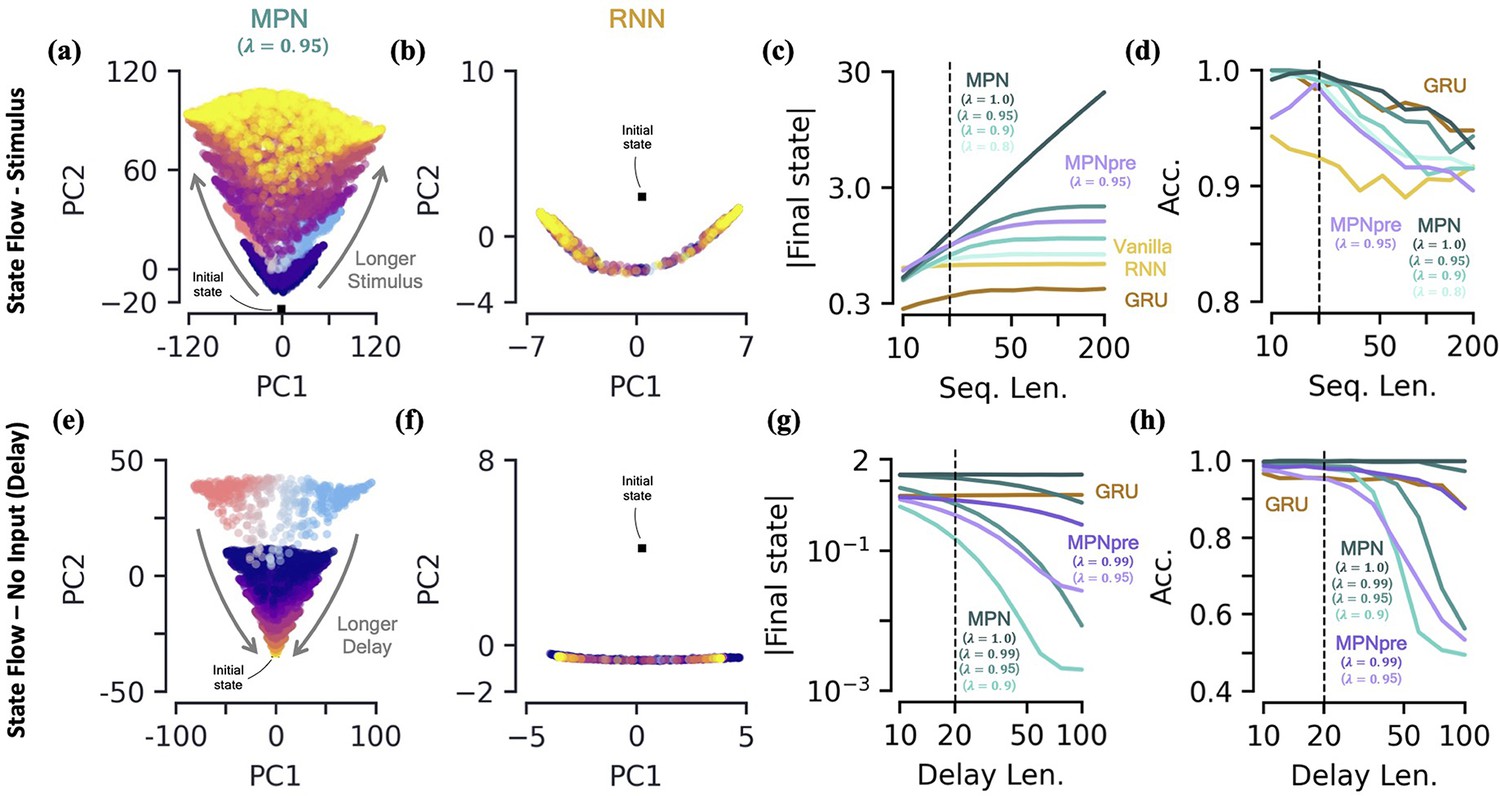
Two-class integration: long-time behavior of multi-plasticity network and RNNs.
[a-d] Flow of states under stimulus. (a) The MPN state, , collected over 100 input sequences, colored by the stimulus length , for (dark blue) to 200 (yellow) time steps, with . The are projected onto their PCA space. The blue/red colored are for and are the same as those in Figure 3f. (b) Same as (a), for the Vanilla RNN states, , plotted in their PCA space. (c) For various sequences lengths, , normalized magnitude of final states. Networks trained on a sequence length of (dotted line). (d) Accuracy of the networks shown in (c) as a function of sequence length. [e-h] Flow of states under zero input (delay input). (e) MPN states, , collected over 100 input sequences, colored by the delay length, 10 (dark blue) to 100 (yellow) time steps. The blue/red colored are for zero delay. (f) Same as (e), for GRU states. (g) For various delay lengths, magnitude of final state. Networks trained with a delay of 20 (dotted line). (h) Accuracy of the networks shown in (i) as a function of delay length.
Figure 5 with 1 supplement
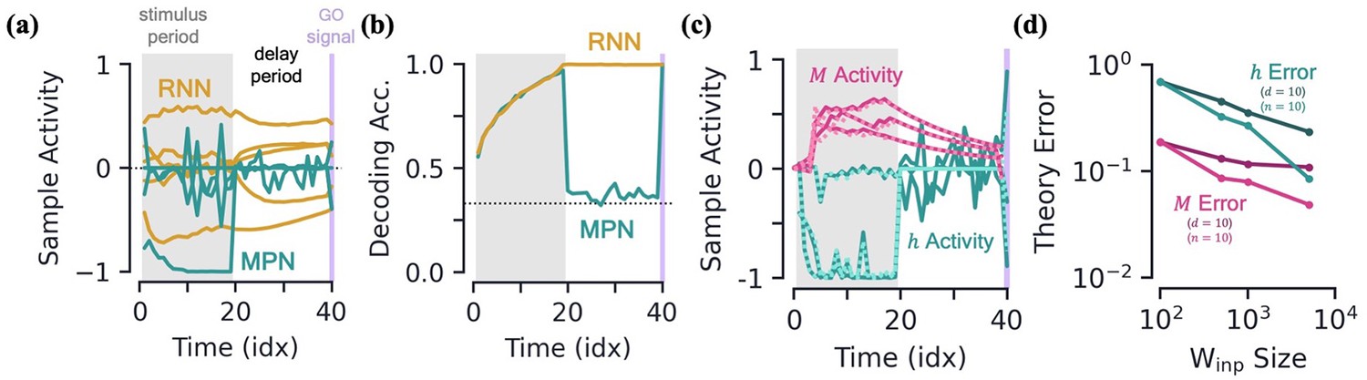
Integration with delay and analytical predictions.
[a-b] MPN and RNN hidden activity behavior during a integration-delay task. The left shaded grey region represents the stimulus period; followed by the delay period with a white background; and finally the thin purple-shaded region representing the response to the go signal. (a) Sample hidden neuron activity for the MPN and RNN. (b) Decoding accuracy on the hidden neuron activity of the MPN and RNN as a function of time (Methods 5.5). Dotted line represents chance accuracy. [c-d] Analytical MPN approximations. (c) Exemplar hidden neuron (teal) and SM matrix (pink) activity as a function of time (solid lines) and their analytical predictions (dotted lines) from Equations 4 and 5. Shading is the same as (a) and (b). (d) Overall accuracy of of theoretical predictions as a function of the size of with either or fixed (Methods 5.5).
Figure 5—figure supplement 1

More on delay dynamics of the MPN and RNN.
[a-c] Various measures as a function of time for networks trained with different delay inputs magnitudes. Note throughout the main text. (a) Mean activity magnitude. (b) Decoding accuracy. (c) Normalized time variance of hidden layer neurons for the MPN and GRU networks (Methods). Variation is measured over a rolling window of previous 5 sequence inputs, so data for first four time steps is omitted. Region of grey-to-white gradient represents transition between stimulus and delay periods, where time window captures data from both periods. (d) Error of theoretical approximations, same as Figure 5d, now as a function of sequence time. [e-g] Cross time decoding accuracy for the GRU and MPN. Color scale is the same for all plots. (e) Decoding accuracy on the hidden neuron activity for a GRU. The and axes show the testing and training times, respectively. For this plot, . (f) Same as (e), for the MPN. (g) Same as (f), but now .
Figure 6 with 1 supplement
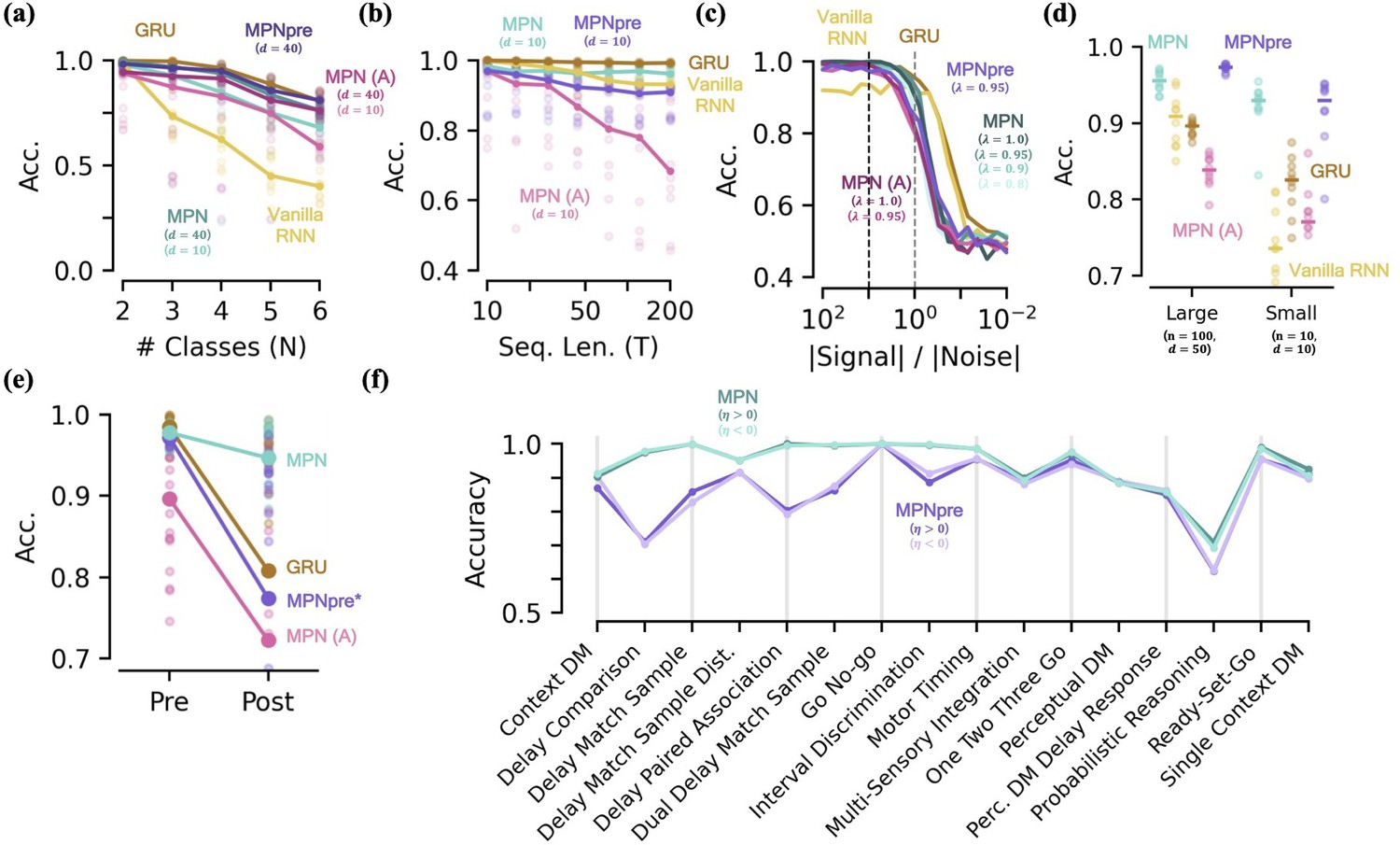
Capacity, robustness, and flexibility of the MPN.
[a-d] Accuracy of the MPN and RNNs as a function of several measures that make the integration task more difficult, see Figure 6—figure supplement 1 for MPNpre results. (a) For very small networks (, ), number of classes in integration task () with fixed sequence length, (Methods 5.5). (b) Also for very small networks, length of integration task () with fixed number of classes, . (c) Ratio of signal and noise magnitudes of the input (Methods 5.5). Networks were trained at a ratio of 10 (dotted black line), the dotted grey line represents a ratio of 1.0. (d) Networks trained with all parameters frozen at initialization values except for readout matrix (and , ). [e-f] Flexibility to learn new tasks. (e) Accuracy on a two-class integration-delay task pre- and post-training on a novel two-class integration-delay task. Thick lines/dots show averages, raw trial data is scattered behind. (f) Hidden activity, colored by sequence label, for a GRU trained on a two-class integration task (red/blue classes) when a novel class (green) is introduced without additional training. Activity collected over 1000 input sequences, plotted in their PCA space. Also shown are readouts, initial state, and sample trajectory. (g) Same as (f), for the MPN state, (h) Decoding accuracy of the final states of the MPN and GRU when a novel class introduced, again without training. Dotted line represents accuracy that would be achieved for perfect classification of only the 2 familiar classes.
Figure 6—figure supplement 1
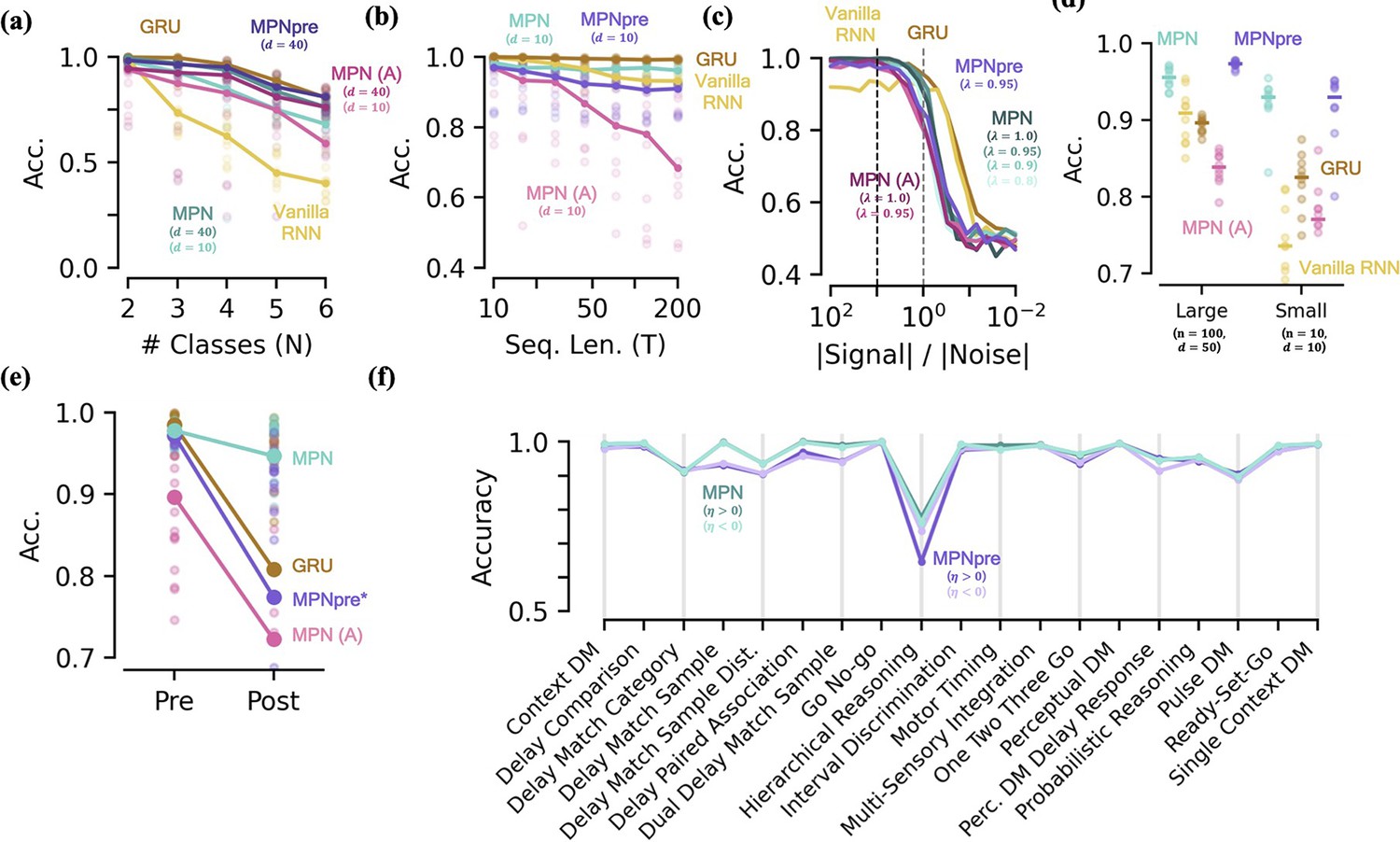
Additional performance comparisons, including additive MPN.
Results here were already partially shown in Figure 6. [a-d] Accuracy of various networks, as a function of several measures that make the integration task more difficult. (a) For very small networks (, , unless otherwise stated), number of classes in integration task () with fixed sequence length, . (b) Also for very small networks, length of integration task () with fixed number of classes, . (c) Ratio of signal to noise magnitudes of the input. Networks were trained at a ratio of 10 (dotted black line), the dotted grey line represents a ratio of 1.0. (d) Networks trained with all parameters frozen at initialization values except for readout matrix (, ). (e) Accuracy on a two-class integration with delay task pre- and post-training on a novel two-class integration task. Thick lines/dots show averages, raw trial data is scattered behind. *The MPNpre has a significantly more difficult time achieving the accuracy threshold on this integration task with a delay period, see Figure 6—figure supplement 1 details for additional discussion. (f) Performance of the MPN and MPNpre for and across 19 supervised learning NeuroGym tasks.
Figure 7 with 1 supplement
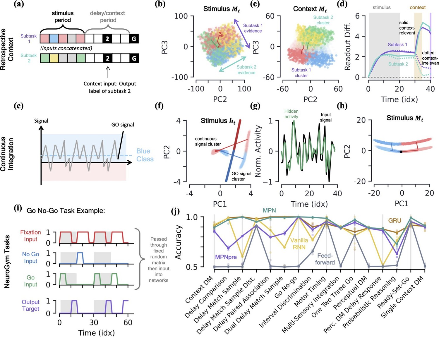
MPN dynamics on additional tasks.
[a-d] Retrospective context task. (a) Schematic of example sequence. (b) MPN states during the initial stimulus period, projected into their (flattened) PCA space, colored by label and subtask (subtask 1: red/blue, subtask 2: green/yellow). Two example trajectories are shown. (c) Same as (b), for states during the time period where the network is passed context (5 time steps). States at end of time period colored darker for clarity. (d) The readout difference of the MPN as a function of sequence time (Methods 5.5). More positive values correspond to the MPN better distinguishing the two classes for the subtask. Solid lines correspond to when the subtask is chosen by the context, dotted lines to when the subtask is not chosen by the context. Grey, yellow, and white background correspond to stimulus, context, and delay periods, respectively. [e-h] Continuous integration task. (e) Schematic of example sequence. (f) Hidden neuron activity, colored by sequence label, projected into their PCA space. Thick lines are readout vectors of corresponding class. (g) Normalized input (black) and example hidden neuron (green) activities, as a function of time (Methods 5.5). (h) MPN states, colored by sequence label, projected into their PCA space. Two example trajectories are shown, black square is the initial state. [i-j] NeuroGym tasks (French, 1999). (i) The beginning of an example sequence of the Go No-Go task. The grey/white shading behind the sequence represents distinct stimulus/delay/decision periods within the example sequence. (j) Performance of the various networks we investigate across 19 supervised learning NeuroGym tasks (Methods 5.5).
Figure 7—figure supplement 1
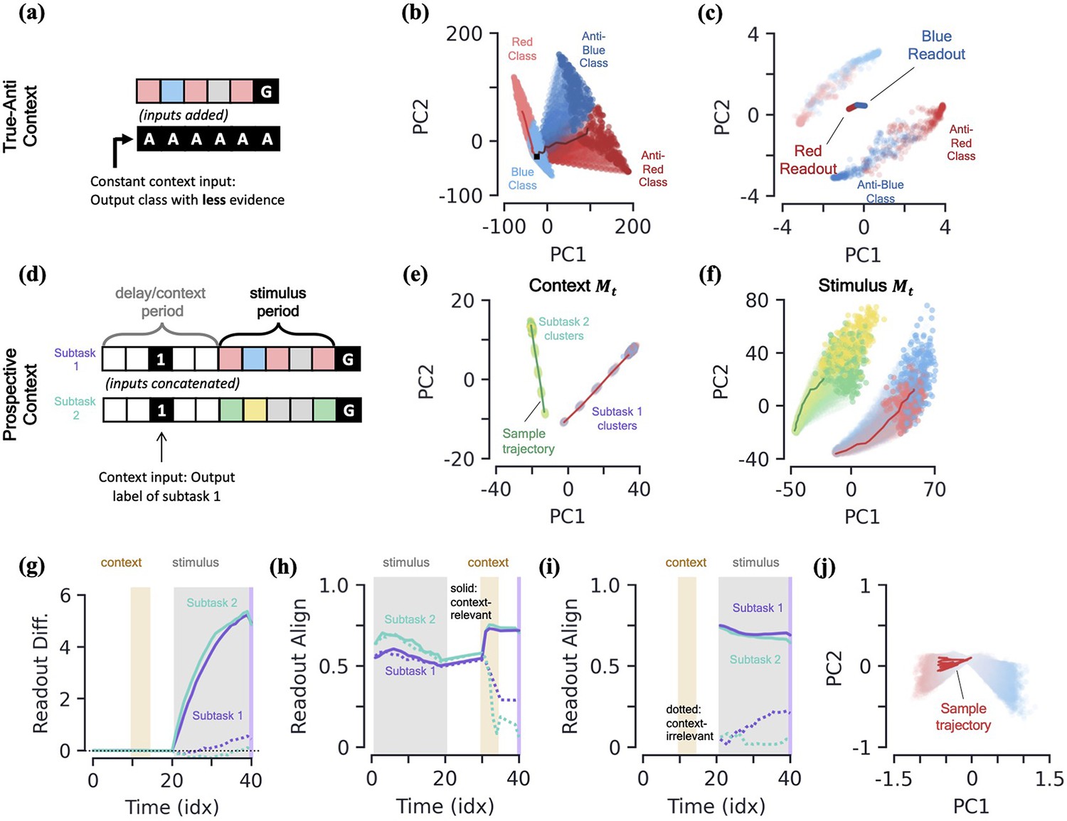
More integration tasks, supplemental figures.
[a-c] True-anti context task. (a) Schematic of example sequence. The context vector, which is passed as an input to the network (added to the regular stimulus inputs), is passed during the entire input sequence. An ‘anti-’ context tells the network to report the class with the least evidence. A ‘true’ context tells the network to solve the task as usual, reporting the class with the most evidence. (b) PC projection of the SM matrix for the entire input sequence, colored by both class label and context. The darker colors represent the SM matrix for ‘anti-’ context cases. (c) Final hidden activity, colored by both class label and context. Also shown are readouts. [d-g] Prospective context task. (d) Schematic of example sequence. (e) MPN states during the initial context period, projected into their (flattened) PCA space, colored by label and subtask (subtask 1: red/blue, subtask 2: green/yellow). Two example trajectories are shown. (f) Same as (f), for states during the time period where the network is passed stimulus information. States at end of time period colored darker for clarity. (g) The readout difference of the MPN as a function of sequence time (Methods 5.5). More positive values correspond to the MPN better distinguishing the two classes for the subtask. Solid lines correspond to when the subtask is chosen by the context, dotted lines to when the subtask is not chosen by the context. Grey, yellow, and white background correspond to stimulus, context, and delay periods, respectively. [h-i] Readout alignment with subtask evidence variation as a function of time (Methods). (h) Retrospective context case. Solid lines correspond to relevant subtask, dotted line to irrelevant subtask. Notably, the alignment of the readouts and variation plummets for the irrelevant task when the context is passed to the network. (i) Prospective context. Alignment is only shown after evidence is passed to the network because subtask evidence variation is ill-defined prior to evidence stimuli. (j) Closeup of the hidden activity for the stimulus period (prior to the go signal) for the continuous integration task shown in Figure 2j.
Tables
Table 1
Parameter and operation counts for various networks.
The number of neurons in the input, hidden, and output layers are , , and , respectively. Note these counts do not include parameters of the readout layer, since said layer contributes the same number of parameters for each network ( and with and without a bias) and are for fixed initial states.
| Network | Trainable Parameters | State update operations |
|---|---|---|
| 2-layer fully connected | ||
| MPN | ||
| MPNpre | ||
| Vanilla RNN | ||
| GRU | ||
| LSTM |
Additional files
Download links
A two-part list of links to download the article, or parts of the article, in various formats.
Downloads (link to download the article as PDF)
Open citations (links to open the citations from this article in various online reference manager services)
Cite this article (links to download the citations from this article in formats compatible with various reference manager tools)
Neural population dynamics of computing with synaptic modulations
eLife 12:e83035.
https://doi.org/10.7554/eLife.83035


