Research Article

Neuroscience

Neural assemblies uncovered by generative modeling explain whole-brain activity statistics and reflect structural connectivity

Computational Neuroscience Lab, Department of Neurophysiology, Donders Center for Neuroscience, Radboud University, Netherlands
Sorbonne Université, CNRS, Institut de Biologie Paris-Seine (IBPS), Laboratoire Jean Perrin (LJP), France
Department of Physiology, Anatomy and Genetics, University of Oxford, United Kingdom
Blavatnik School of Computer Science, Tel Aviv University, Israel
Department Genes – Circuits – Behavior, Max Planck Institute for Biological Intelligence, Germany
Allen Institute for Brain Science, United States

Jan 17, 2023

https://doi.org/10.7554/eLife.83139

Open access
Copyright information

Version of Record

Accepted for publication after peer review and revision.

Download
Cite
Share
CommentOpen annotations (there are currently 0 annotations on this page).

Version of Record published: February 20, 2023 (This version)
Accepted Manuscript published: January 17, 2023 (Go to version)
Accepted: January 15, 2023
Received: September 21, 2022
Preprint posted: November 11, 2021 (Go to version)

Figures
Videos
Tables
Additional files

6 figures, 1 video, 1 table and 3 additional files

Figures

Figure 1

Download asset Open asset

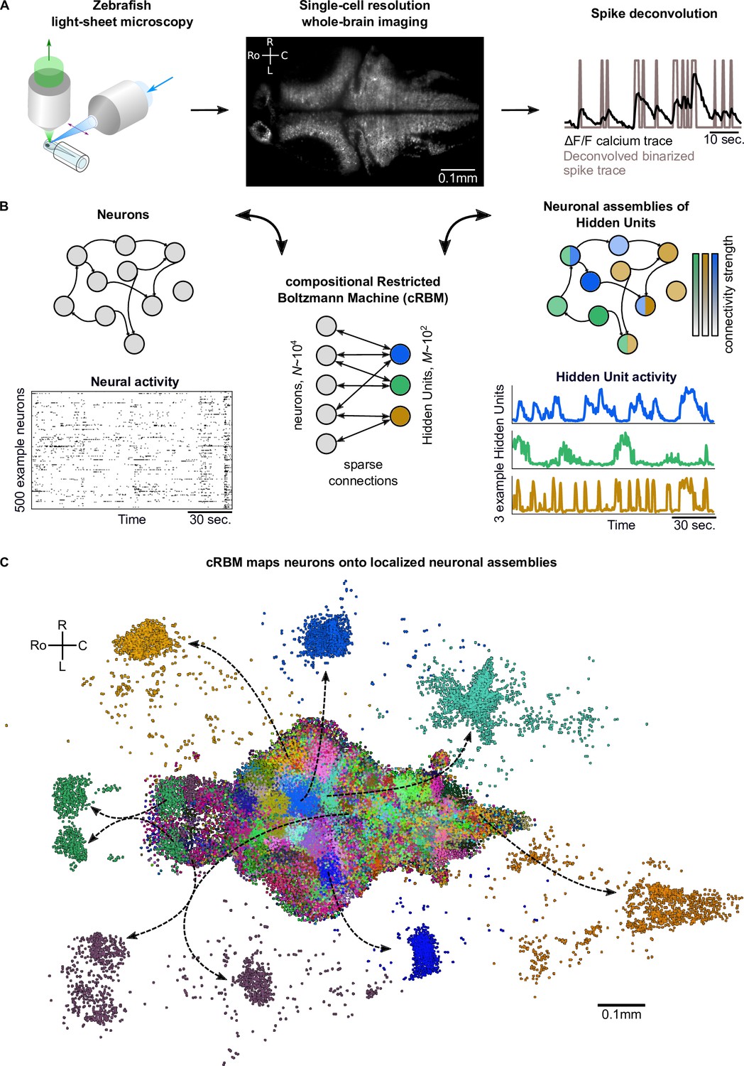
cRBMs construct Hidden Units by grouping neurons into assemblies.

(A) The neural activity of zebrafish larvae was imaged using light-sheet microscopy (left), which resulted in brain-scale, single-cell resolution data sets (middle, microscopy image of a single plane shown for fish #1). Calcium activity $Δ F / F$ was deconvolved to binarized spike traces for each segmented cell (right, example neuron). (B) cRBM sparsely connects neurons (left) to Hidden Units (HUs, right). The neurons that connect to a given HU (and thus belong to the associated assembly), are depicted by the corresponding color labeling (right panel). Data sets typically consist of $N \sim 10^{4}$ neurons and $M \sim 10^{2}$ HUs. The activity of 500 randomly chosen example neurons (raster plot, left) and HUs 99, 26, 115 (activity traces, right) of the same time excerpt is shown. HU activity is continuous and is determined by transforming the neural activity of its assembly. (C) The neural assemblies of an example data set (fish #3) are shown by coloring each neuron according to its strongest-connecting HU. 7 assemblies are highlighted (starting rostrally at the green forebrain assembly, going clockwise: HU 177, 187, 7, 156, 124, 64, 178), by showing their neurons with a connection $| w | \geq 0.1$ . See Figure 3 for more anatomical details of assemblies. R: Right, L: Left, Ro: Rostral, C: Caudal.

Figure 2 with 7 supplements

Download asset Open asset

cRBM is optimized to accurately replicate data statistics.

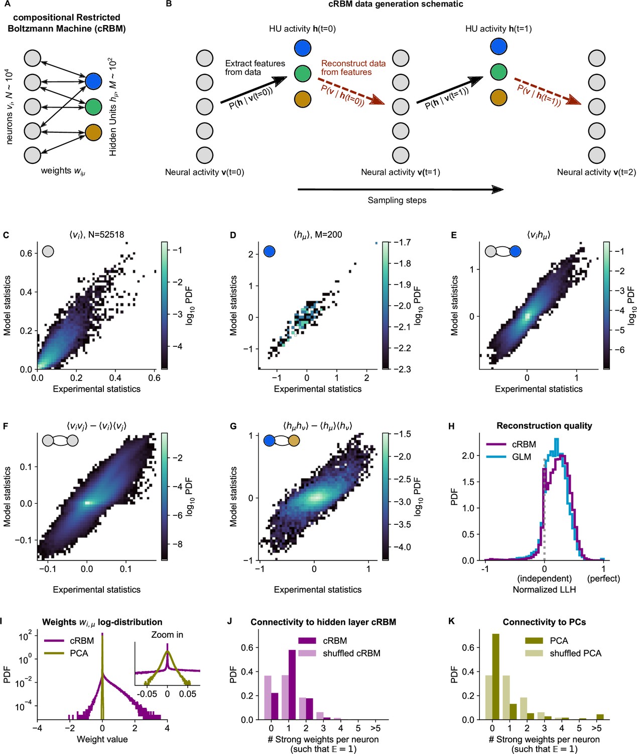
(A) Schematic of the cRBM architecture, with neurons $v_{i}$ on the left, HUs $h_{μ}$ on the right, connected by weights $w_{i, μ}$ . (B) Schematic depicting how cRBMs generate new data. The HU activity $h (t)$ is sampled from the visible unit (i.e. neuron) configuration $v (t)$ , after which the new visible unit configuration $v (t + 1)$ is sampled and so forth. (C) cRBM-predicted and experimental mean neural activity $⟨ v_{i} ⟩$ were highly correlated (Pearson correlation $r_{P} = 0.91$ , $P < 10^{- 307}$ ) and had low error ( ${nRMSE}_{⟨ v_{i} ⟩} = 0.11$ , normalized Root Mean Square Error, see Materials and methods - ‘Calculating the normalized Root Mean Square Error’ ). Data displayed as 2D probability density function (PDF), scaled logarithmically (base 10). (D) cRBM-predicted and experimental mean Hidden Unit (HU) activity $⟨ h_{μ} ⟩$ also correlated very strongly ( $r_{P} = 0.93$ , $P < 10^{- 86}$ ) and had low ${nRMSE}_{⟨ h_{μ} ⟩} = 0.15$ (other details as in C) (E) cRBM-predicted and experimental average pairwise neuron-HU interactions $⟨ v_{i} h_{μ} ⟩$ correlated strongly ( $r_{P} = 0.74$ , $P < 10^{- 307}$ ) and had a low error ( ${nRMSE}_{⟨ v_{i} h_{μ} ⟩} = 0.09$ ). (F) cRBM-predicted and experimental average pairwise neuron-neuron interactions $⟨ v_{i} v_{j} ⟩$ correlated well ( $r_{P} = 0.58$ , $P < 10^{- 307}$ ) and had a low error ( ${nRMSE}_{⟨ v_{i} v_{j} ⟩} = - 0.09$ , where the negative nRMSE value means that cRBM-predictions match the test data slightly better than the train data). Pairwise interactions were corrected for naive correlations due to their mean activity by subtracting $⟨ v_{i} ⟩ ⟨ v_{j} ⟩$ . (G) cRBM-predicted and experimental average pairwise HU-HU interactions $⟨ h_{μ} h_{ν} ⟩$ correlated strongly ( $r_{P} = 0.73$ , $P < 10^{- 307}$ ) and had a low error ( ${nRMSE}_{⟨ h_{μ} h_{ν} ⟩} = 0.17$ ). (H) The low-dimensional cRBM bottleneck reconstructs most neurons above chance level (purple), quantified by the normalized log-likelihood (nLLH) between neural test data v_i and the reconstruction after being transformed to HU activity (see Materials and methods - ‘Reconstruction quality’). Median normalized = ${nLLH}_{cRBM}$ 0.24. Reconstruction quality was also determined for a fully connected Generalized Linear Model (GLM) that attempted to reconstruct the activity of a neuron v_i using all other neurons $v_{- i}$ (see Materials and methods - ‘Generalized Linear Model’). The distribution of 5000 randomly chosen neurons is shown (blue), with median ${nLLH}_{GLM} = 0.20$ . The cRBM distribution is stochastically greater than the GLM distribution (one-sided Mann Whitney U test, $P < 10^{- 42}$ ). (I) cRBM (purple) had a sparse weight distribution, but exhibited a greater proportion of large weights $w_{i, μ}$ than PCA (yellow), both for positive and negative weights, displayed in log-probability. (J) Distribution of above-threshold absolute weights $| w_{i, μ} |$ per neuron v_i (dark purple), indicating that more neurons strongly connect to the cRBM hidden layer than expected by shuffling the weight matrix of the same cRBM (light purple). The threshold $Θ$ was set such that the expected number of above-threshold weights per neuron $E (# w_{i} > Θ) = 1$ . (K) Corresponding distribution as in (J) for PCA (dark yellow) and its shuffled weight matrix (light yellow), indicating a predominance of small weights in PCA for most neurons v_i. All panels of this figure show the data statistics of the cRBM with parameters $M = 200$ and $λ = 0.02$ (best choice after cross-validation, see Figure 2—figure supplement 1) of example fish #3, comparing the experimental test data test and model-generated data after cRBM training converged.

Figure 2—figure supplement 1

Download asset Open asset

cRBM free parameter optimization by cross-validation.

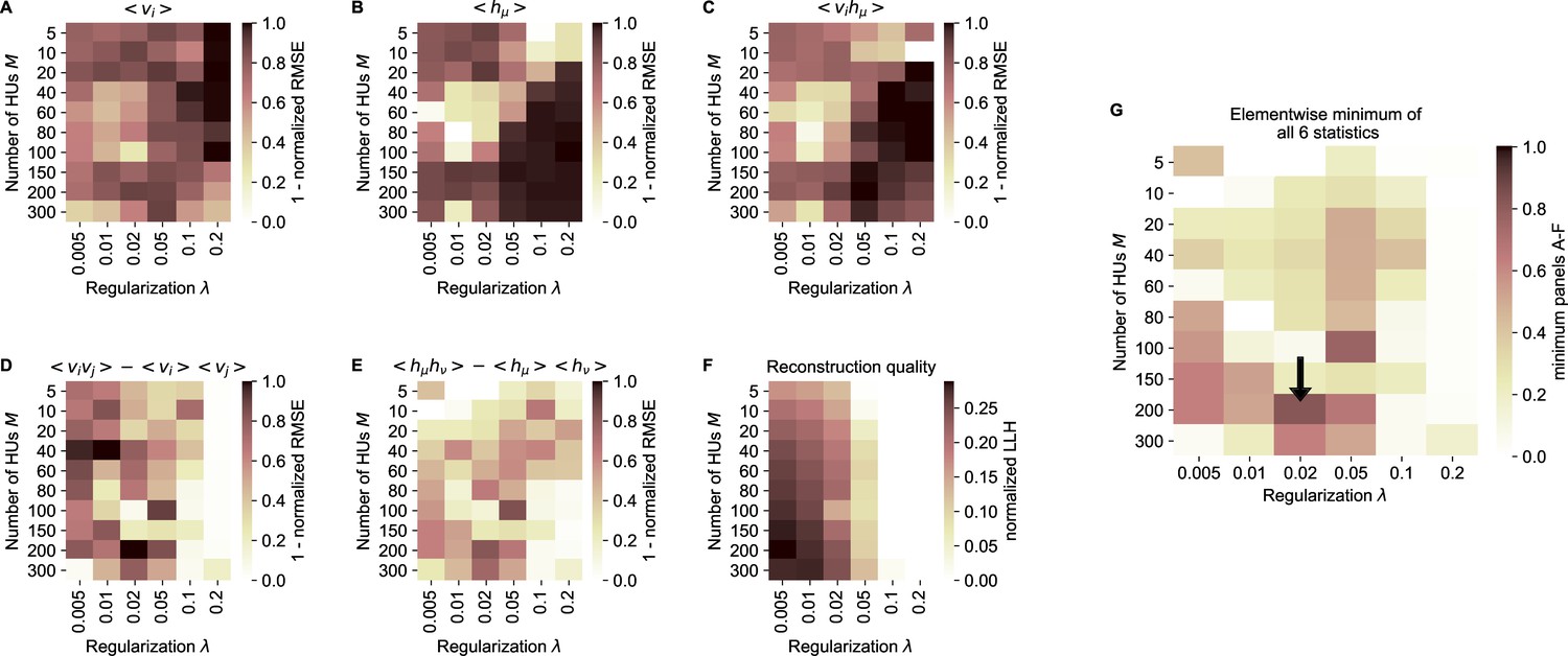
(A) Model performance, as quantified by the normalized RMSE (nRMSE, see Materials and methods - ‘Calculating the normalized root mean square error’) of the mean neural activity $⟨ v_{i} ⟩$ , as a function of the sparsity regularization parameter $λ$ (x-axis) and the number of HUs $M$ (y-axis). cRBM models were evaluated after training converged on withheld testing data. $1 - nRMSE$ values are shown to enable optimization by maximization in panel G. Values below 0 were set to 0 for panels A-F. (B) Equivalent figure for the mean HU activity $⟨ h_{μ} ⟩$ . (C) Equivalent figure for average pairwise neuron-HU interactions $⟨ v_{i} h_{μ} ⟩$ . (D) Equivalent figure for average pairwise neuron-neuron interactions $⟨ v_{i} v_{j} ⟩$ . (E) Equivalent figure for average pairwise HU-HU interactions $⟨ h_{μ} h_{ν} ⟩$ . (F) Equivalent figure for the reconstruction quality of the low-dimensional cRBM bottleneck, quantified by the median normalized LLH. (G) The cRBM free parameters were optimized by maximizing the element-wise minimum of panels A-F. Using the element-wise minimum to compare the six statistics ensures that the model performs performs well on all aspects. First, in order to compare panels A-E with panel F, the values of panel F were scaled to 1 by dividing all elements of panel F by its maximum value (=0.29). Next, for each $(λ, M)$ combination the minimum value was determined from all 6 evaluation criteria. These are shown in this panel, with the black arrow indicating the resulting maximum of 0.83 at $(λ = 0.02, M = 200)$ .

Figure 2—figure supplement 2

Download asset Open asset

Generalized Linear Model (GLM) parameter optimization.

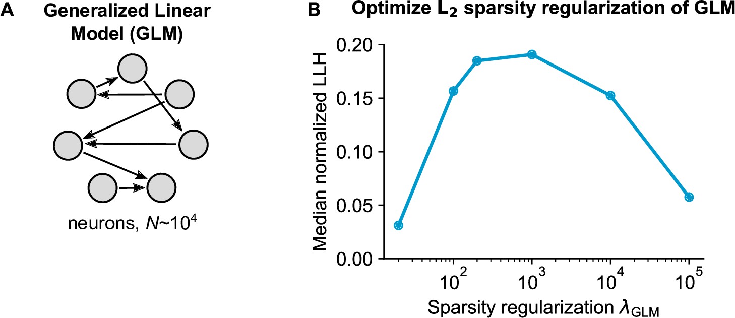
(A) Schematic of the pairwise GLM model. Connections were estimated with logistic regression and L₂ sparsity regularization. (B) The sparsity regularization parameter $λ_{GLM}$ was optimized using cross-validation of 6 parameter configurations, using 1000 randomly sampled neurons.

Figure 2—figure supplement 3

Download asset Open asset

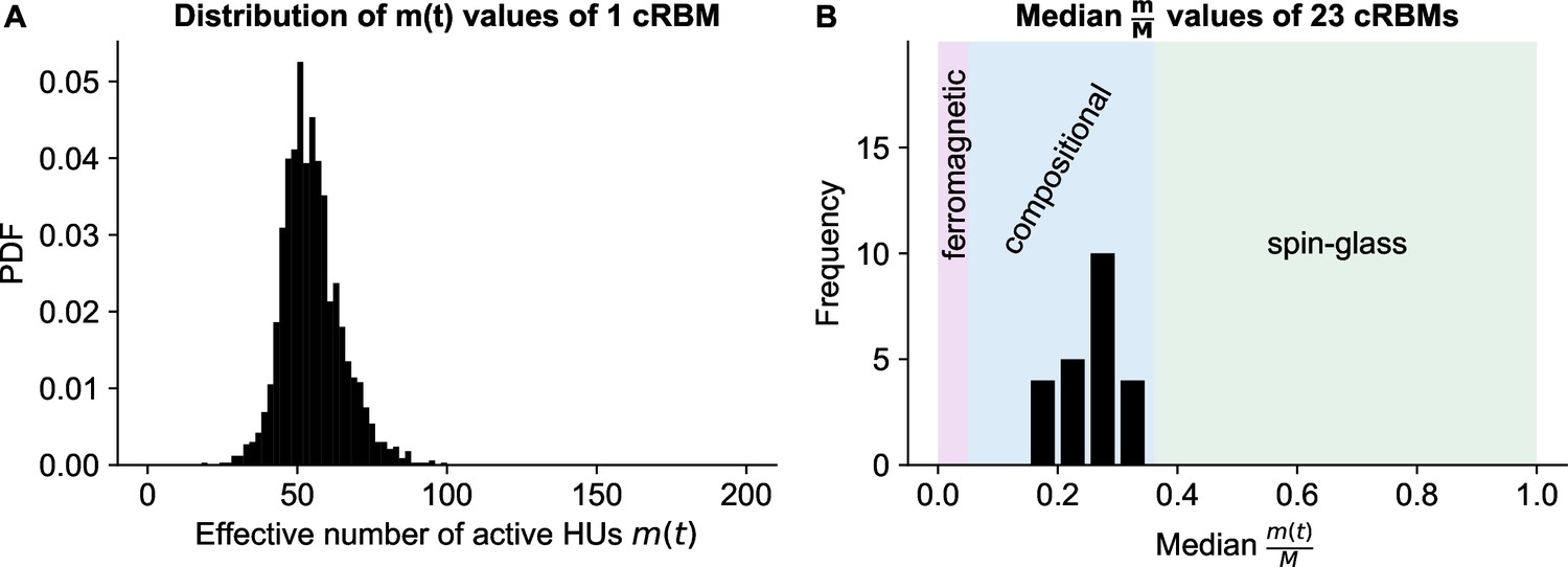
cRBMs are in the compositional phase after convergence.

(A) Distribution of $m (t)$ , the number of effective active HUs per time point $t$ , calculated on the test data of example fish #3. $m (t)$ is defined as $m (t) = PR (h_{+} (t)) \cdot M$ , where PR is the Participation Ratio (Equation 19). Median $m (t) = 0.27 \cdot M = 54$ . (B) The distribution of median $\frac{m (t)}{M}$ values of the entire recordings of all cRBMs used for the connectivity analyses. The average $\frac{median (m)}{M}$ across all cRBMs is 0.26. The compositional phase is characterized by $1 ≪ m (t) ≪ M$ which occurs for all cRBMs. The three phases are indicated. Here, the ferromagnetic phase upper bound was manually set at 5%, and the spin-glass phase lower bound was determined by computing the PR of normally distributed activity (with mean and standard deviation of the test data of example fish #3 of panel A).

Figure 2—figure supplement 4

Download asset Open asset

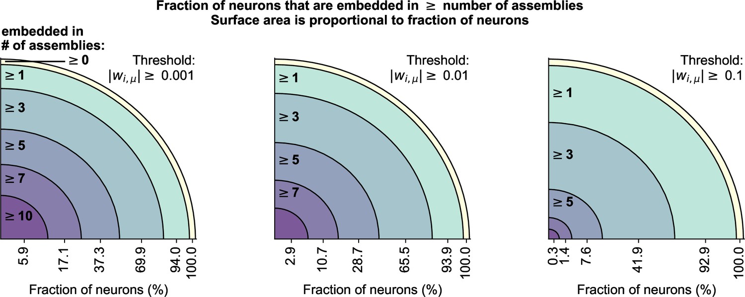
Neurons can be embedded in multiple assemblies.

cRBM allow neurons to be embedded in multiple assemblies, which we quantified by measuring the number of above-threshold weights $| w_{i, μ} | \geq threshold$ per neuron.Threshold values of 0.001 (left), 0.01 (middle), and 0.1 (right) were used. For each threshold value, we counted the fraction of neurons that had at least 0, 1, 3, 5, 7, or 10 above-threshold weights (i.e. were embedded in at least that many assemblies), as denoted on the x-axis of each panel. Changing the threshold from 0.001 to 0.01 did not cause a large shift in the distribution of embedded assemblies (left vs middle), indicating that there were few connections in the range $0.001 \leq w_{i, μ} \leq 0.01$ . Increasing the threshold to 0.1 strongly decreased the number of neurons with many (gt₃) assembly embeddings, but not the number of neurons with at least 1 assembly embedding, indicating that most neurons have at least 1 strong assembly connection (in accordance with Figure 2J).

Figure 2—figure supplement 5

Download asset Open asset

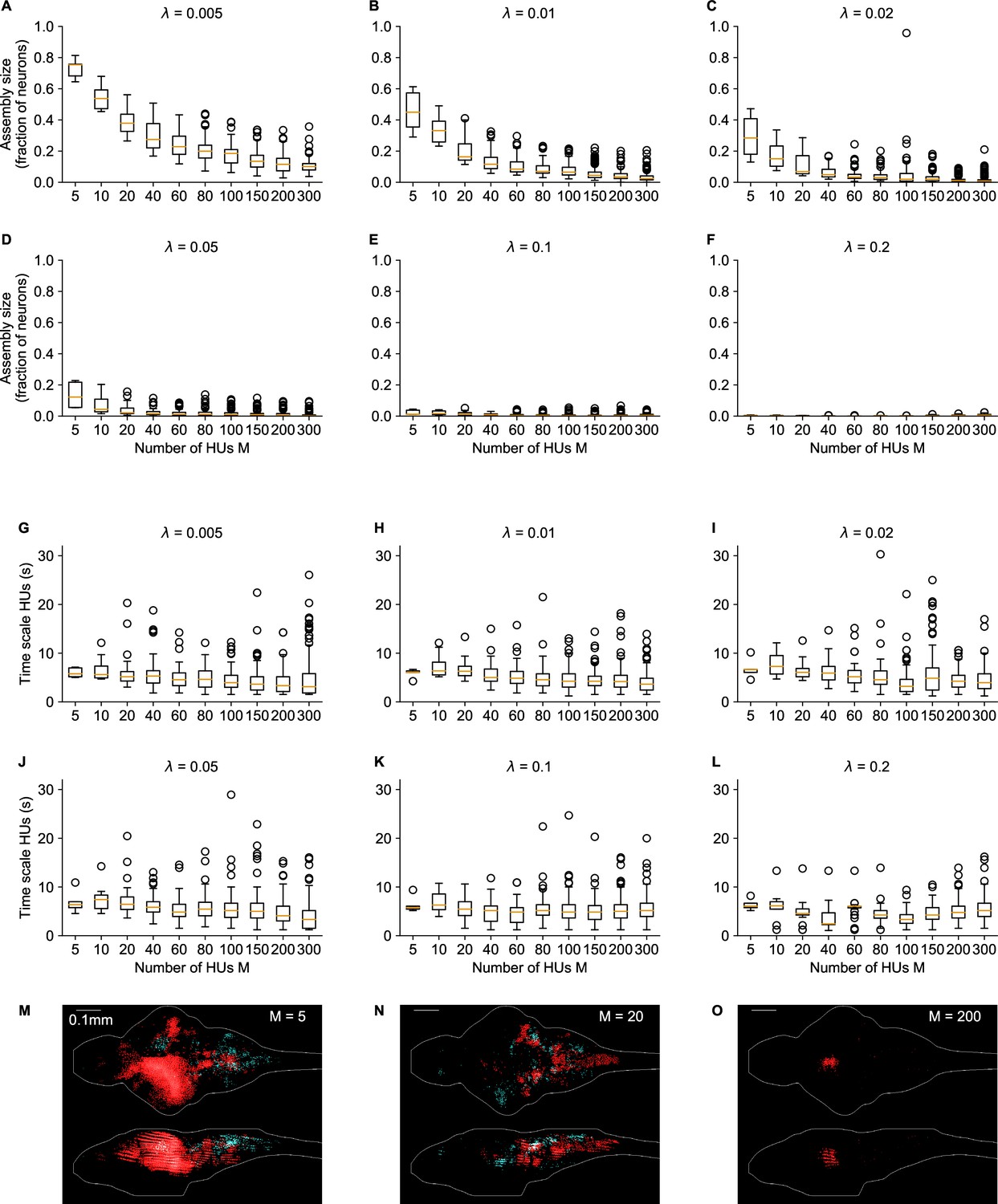
Influence of number of HUs $M$ and sparsity regularization $λ$ on cRBM properties.

(**A–F**) The distribution of assembly sizes is shown as a function of number of HUs $M$ (x-axis) and sparsity regularization parameter $λ$ (panels). Assembly size was determined by computing $\frac{1}{N} \sum_{i}^{N} | w_{i, μ} | > 0.01$ for each HU μ. Two-way ANOVA determined that both $M$ ( $P = 7 \cdot 10^{- 6}$ ) and $λ$ ( $P = 4 \cdot 10^{- 4}$ ), as well as their interaction ( $P = 7 \cdot 10^{- 3}$ ) significantly explained the mean assembly size. (**G–L**) The distribution of HU dynamics time scales is shown as a function of $M$ (x-axis) and $λ$ (panels). Time scales were calculated as in Figure 2F. There are 2 extra out-of-panel outliers for $M = 150, λ = 0.05$ at 70 s and $M = 300, λ = 0.05$ at 36 s. Two-way ANOVA determined that only $M$ ( $P = 7 \cdot 10^{- 8}$ ) strongly significantly explained the mean time scale, while $λ$ ( $P = 0.2$ ) did not and their interaction ( $P = 0.01$ ) only weakly. M-O Three example assemblies are shown, corresponding to the mean assembly size of $M = 5$ (panel M), $M = 20$ (N) and $M = 200$ (O) cRBM models (all with $λ = 0.02$ ). Assembly sizes are 0.27 (M), 0.07 (N), 0.01 (O), respectively.

Figure 2—figure supplement 6

Download asset Open asset

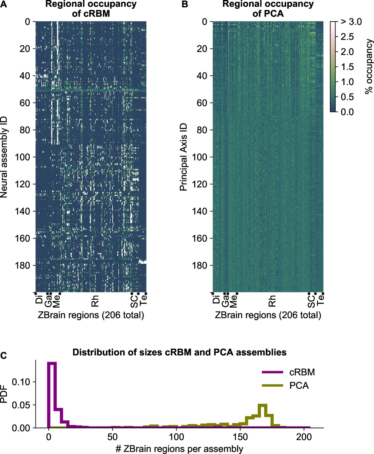
cRBM assemblies are sparse and spatially localized.

(A) For each neural assembly (y-axis), the occupancy of ZBrain Atlas (Randlett et al., 2015) brain regions (x-axis, sorted alphabetically) was determined, by quantifying the number of anatomical regions that each HU connects to (i.e. the overlap between cRBM assemblies and anatomical regions, see Materials and methods - ‘Regional occupancy’). ZBrain atlas regions that were not imaged were excluded, yielding $N_{ZBA} = 206$ regions in total. Occupancy was defined as the dot product between the binary ZBrain-label matrix (size $N_{ZBA} \times N$ , where 1 indicates that a neuron is embedded in an anatomical region, and 0 vice versa) and the cRBM weight matrix (size $N \times M$ ), and was normalized to 100% for each assembly to account for different assembly sizes. Assemblies were sorted by their dynamics (Figure 2B, Materials and methods). ZBrain Atlas regions are abbreviated by: Diencephalon (Di), Ganglia (Ga), Mesencephalon (Me), Rhombencephalon (Rh), Spinal Cord (SC) and Telencephalon (Te). (B) Equivalent figure for Principal Axes of PCA (i.e. the PCA Eigenvectors). Principal Axes were sorted by Eigenvalue. Panels A and B share the same color scale (right). (C) Distributions of the effective number of ZBrain Atlas regions per assembly (Principal Axis) of the occupancy metric of panel A (B) for cRBM (PCA), respectively. The effective number of regions was determined by calculating the Participation Ratio per assembly (Principal Axis), multiplied with the total number of regions $N_{ZBA}$ (see Materials and methods - ‘Regional occupancy’). cRBM assemblies occupy a median of 3 regions (interquartile range: 2–6 regions), while PCA assemblies occupy a median of 160 regions (interquartile range: 140–168 regions).

Figure 2—figure supplement 7

Download asset Open asset

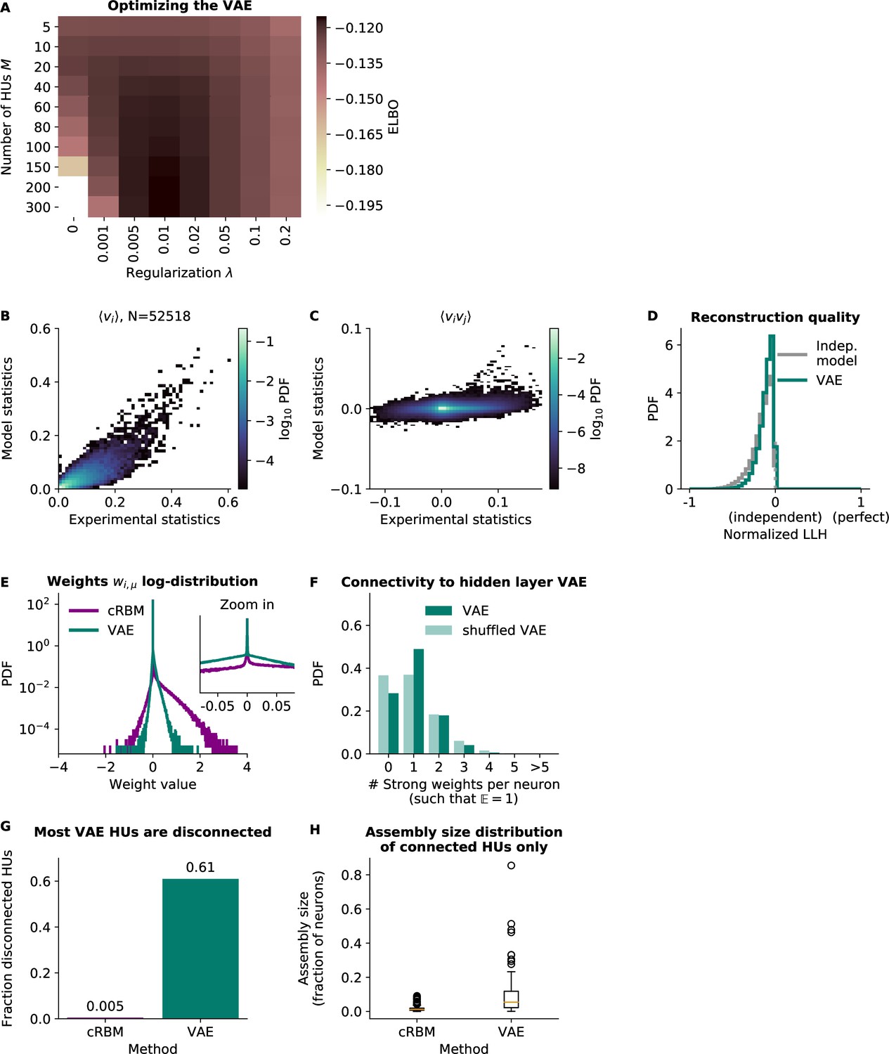
Variational Autoencoder (VAE) models do not fit the second-order statistics of the neural data.

(A) VAE model performance, quantified by its ELBO objective on withheld test data. The optimal VAE was found with parameters $M = 300, λ = 0.01$ , and this optimum was very close to the performance of $M = 200, λ = 0.02$ (the cRBM optimal parameters, see Figure 2—figure supplement 1). For ease of comparison, in the other panels we consider the latter VAE model, but also quantify the performance of the first in panels B and C. (B) VAE-predicted and experimental mean neural activity $⟨ v_{i} ⟩$ were strongly correlated Pearson correlation ( $r_{P} = 0.84$ , $P < 10^{- 307}$ ) but still had fairly high error ( ${nRMSE}_{⟨ v_{i} ⟩} = 0.61$ ), presumably because the model appeared to underestimate the activity of most neurons (linear regression determined the optimal slope to be 0.52). The $M = 300, λ = 0.01$ (optimal) VAE model had a similar ${nRMSE}_{⟨ v_{i} ⟩} = 0.54$ . (C) VAE-predicted and experimental average pairwise neuron-neuron interactions $⟨ v_{i} v_{j} ⟩$ had a very high error of ${nRMSE}_{⟨ v_{i} v_{j} ⟩} = 1.23$ , demonstrating that the VAE did not capture the second-order statistics of the data at all. The $M = 300, λ = 0.01$ (optimal) VAE model had a similar ${nRMSE}_{⟨ v_{i} v_{j} ⟩} = 1.22$ . (D) Reconstruction quality of VAE was also very low, performing almost equal to an independent model. (E) VAE weights were similarly sparsely distributed to cRBM weights. (VAE weights were also sign-swapped for consistency with cRBM, see Materials and methods - ‘Choice of HU potential’) (F) The distribution of above-threshold absolute weights was also similar to cRBM (Figure 2J). (G) Fraction of disconnected HUs of cRBM and VAE (defined for each HU μ by $| w_{i, μ} | \leq 0.01 \forall i)$ . (H) Distribution of assembly sizes (determined by $\frac{1}{N} \sum_{i}^{N} | w_{i, μ} | > 0.01$ ), excluding all disconnected HUs (1/200 for cRBM, 122/200 for VAE).

Figure 3

Download asset Open asset

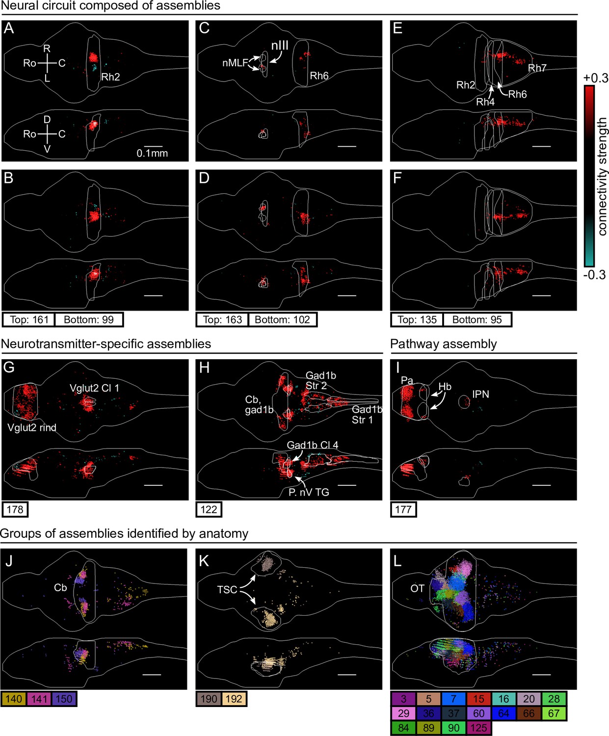
cRBM assemblies compose functional circuits and anatomical structures.

(**A–I**) Individual example assemblies μ are shown by coloring each neuron $i$ with its connectivity weight value $w_{i, μ}$ (see color bar at the right hand side). The assembly index μ is stated at the bottom of each panel. The orientation and scale are given in panel A (Ro: rostral, C: caudal, R: right, L: left, D: dorsal, V: ventral). Anatomical regions of interest, defined by the ZBrain Atlas (Randlett et al., 2015), are shown in each panel (Rh: rhombomere, nMLF: nucleus of the medial longitudinal fascicle; nIII: oculomotor nucleus nIII, Cl: cluster; Str: stripe, P. nV TG: Posterior cluster of nV trigeminal motorneurons; Pa: pallium; Hb: habenula; IPN: interpeduncular nucleus). (**J–L**) Groups of example assemblies that lie in the same anatomical region are shown for cerebellum (Cb), torus semicircularis (TSC), and optic tectum (OT). Neurons i were defined to be in an assembly μ when $| w_{i, μ} | > 0.15$ , and colored accordingly. If neurons were in multiple assemblies shown, they were colored according to their strongest-connecting assembly.

Figure 4

Download asset Open asset

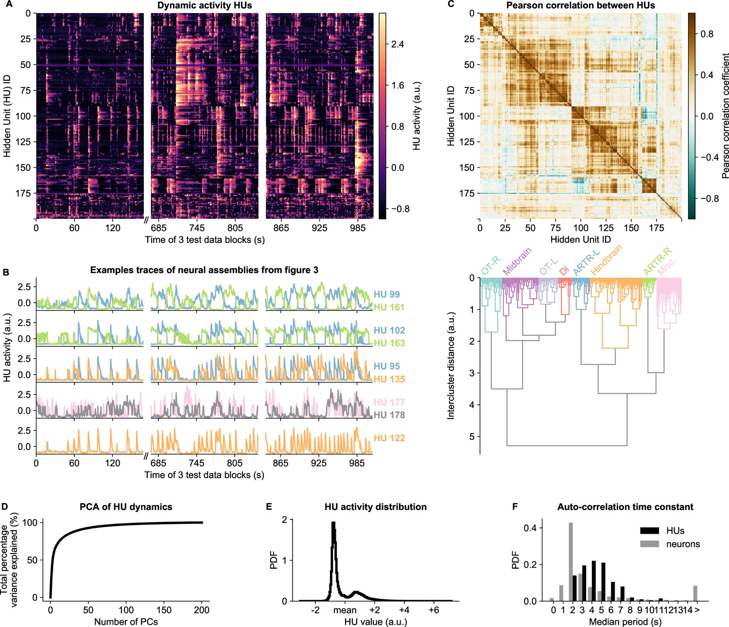
HU dynamics are bimodal and activate slower than neurons.

(A) HU dynamics are diverse and are partially shared across HUs. The bimodality transition point of each HU was determined and subtracted individually, such that positive values correspond to HU activation (see Materials and methods - ‘Time constant calculation’6.12). The test data consisted of three blocks, with a discontinuity in time between the first and second block (Materials and methods). (B) Highlighted example traces from panel A. HU indices are denoted on the right of each trace, colored according to their cluster from panel D. The corresponding cellular assemblies of these HU are shown in Figure 3A-I. (C) Top: Pearson correlation matrix of the dynamic activity of panel A. Bottom: Hierarchical clustering of the Pearson correlation matrix. Clusters (as defined by the colors) were annotated manually. This sorting of HUs is maintained throughout the manuscript. OT: Optic Tectum, Di: Diencephalon, ARTR: ARTR-related, Misc.: Miscellaneous, L: Left, R: Right. (D) A Principal Component Analysis (PCA) of the HU dynamics of panel A shows that much of the HU dynamics variance can be captured with a few PCs. The first 3 PCs captured 52%, the first 10 PCs captured 73% and the first 25 PCs captured 85% of the explained variance. (E) The distribution of all HU activity values of panel A shows that HU activity is bimodal and sparsely activated (because the positive peak is smaller than the negative peak). PDF: Probability Density Function. (F) Distribution of the time constants of HUs (black) and neurons (grey). Time constants are defined as the median oscillation period, for both HUs and neurons. An HU oscillation is defined as a consecutive negative and positive activity interval. A neuron oscillation is defined as a consecutive interspike-interval and spike-interval (which can last for multiple time steps, for example see Figure 1A). The time constant distribution of HUs is greater than the neuron distribution (Mann Whitney U test, $P < 10^{- 16}$ ).

Figure 5 with 1 supplement

Download asset Open asset

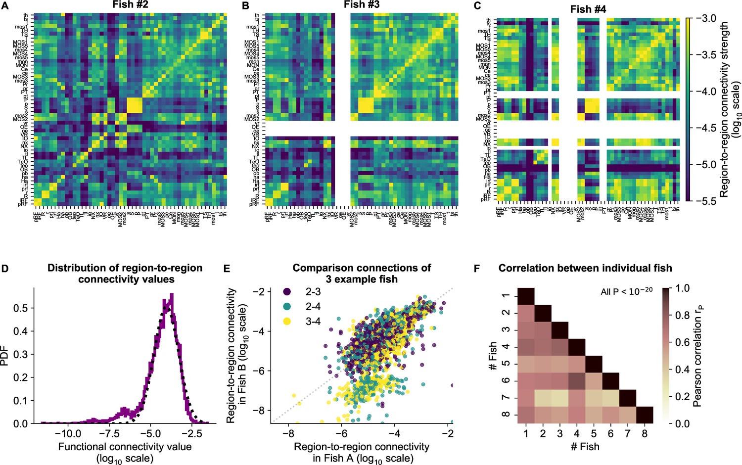
cRBM gives rise to functional connectivity that is strongly correlated across individuals.

(A) The functional connectivity matrix between anatomical regions of the mapzebrain atlas (Kunst et al., 2019) of example fish #2 is shown. Functional connections between two anatomical regions were determined by the similarity of the HUs to which neurons from both regions connect to (Materials and methods). Mapzebrain atlas regions with less than five imaged neurons were excluded, yielding $N_{MAP} = 50$ regions in total. See Supplementary file 1 for region name abbreviations. The matrix is shown in *log*₁₀ scale, because functional connections are distributed approximately log-normal (see panel D). (B) Equivalent figure for example fish #3 (example fish of prior figures). (C) Equivalent figure for example fish #4. Panels A-C share the same *log*₁₀ color scale (right). (D) Functional connections are distributed approximately log-normal. (Mutual information with a log-normal fit (black dashed line) is 3.83, while the mutual information with a normal fit is 0.13). All connections of all eight fish are shown, in *log*₁₀ scale (purple). (E) Functional connections of different fish correlate well, exemplified by the three example fish of panels A-C. All non-zero functional connections (x-axis and y-axis) are shown, in *log*₁₀ scale. Pearson correlation $r_{P}$ between pairs: $r_{P} (# 2, # 3) = 0.73$ , $r_{P} (# 2, # 4) = 0.73$ , $r_{P} (# 3, # 4) = 0.78$ . All correlation p values $< 10^{- 20}$ (two-sided t-test). (F) Pearson correlations $r_{P}$ of region-to-region functional connections between all pairs of 8 fish. For each pair, regions with less than five neurons in either fish were excluded. All p values $< 10^{- 20}$ (two-sided t-test), and average correlation value is 0.69.

Figure 5—figure supplement 1

Download asset Open asset

Functional connectivity matrices of all fish.

8 panels. (**A–H**) showing the individual cRBM functional connectivity matrices of all zebrafish recordings. Panels B, C, and D correspond to Figure 3A–C. All matrices share the same *log*₁₀ color scale (bottom right). Regions that contained less than five neurons were left blank, for each fish individually.

Figure 6 with 1 supplement

Download asset Open asset

cRBM-inferred functional connectivity reflects structural connectivity.

(A) Structural connectivity matrix is shown in *log*₁₀ scale, updated from Figure 8C of Kunst et al., 2019. Regions that were not imaged in our experiments were excluded (such that $N_{MAP} = 50$ out of 72 regions remain). Regions (x-axis and y-axis) were sorted according to Kunst et al., 2019. Compared to Figure 8C of Kunst et al., 2019 additional structural data was added and the normalization procedure was updated to include within-region connectivity (see Materials and methods - ‘Extensions of the structural connectivity matrix’). See Supplementary file 1 for region name abbreviations. (B) Average functional connectivity matrix is shown in *log*₁₀ scale, as determined by averaging the cRBM functional connectivity matrices of all 8 fish (see Materials and methods - ‘Specimen averaging of connectivity matrices’). The same regions (x-axis and y-axis) are shown as in panel A. (C) The average functional and structural connectivity of panels A and B correlate well, with Spearman correlation $r_{S} = 0.39$ ( $P < 10^{- 20}$ , two-sided t-test). Each data point corresponds to one region-to-region pair. Data points for which the structural connection was exactly 0 were excluded (see panel D for their analysis). (D) The distribution of average functional connections of region pairs with non-zero structural connections is greater than functional connections corresponding to region pairs without structural connections ( $P < 10^{- 15}$ , two-sided Kolmogorov-Smirnov test). The bottom panel shows the evidence for inferring either non-zero or zero structural connections, defined as the fraction between the PDFs of the top panel (fitted Gaussian distributions were used for denoising).

Figure 6—figure supplement 1

Download asset Open asset

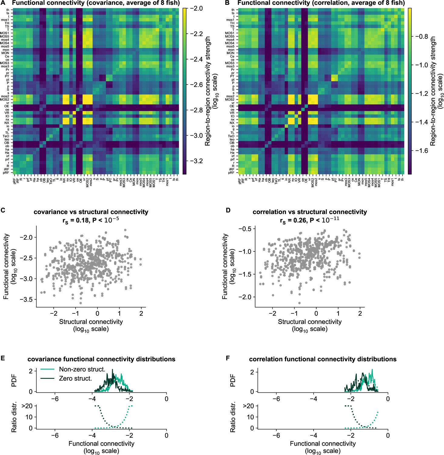
cRBM functional connectivity compared to baseline methods.

(A) Average functional connectivity matrix of the covariance baseline method (see Materials and methods - ‘Connectivity inference baselines’) in *log*₁₀ scale. (B) Average functional connectivity matrix of the Pearson correlations baseline method (see Materials and methods - ‘Connectivity inference baselines’) in *log*₁₀ scale. (**C, D**) Equivalent figure to Figure 4C for functional connections as determined by the covariance (C) and correlations (D) between neurons (see Materials and methods - ‘Correlation analysis of connectivity matrices’). The Spearman correlation coefficient between functional and structural connections for covariance is $r_{S} = 0.18$ and for correlation $r_{S} = 0.26$ . (**E–F**) Equivalent figure to Figure 4D for functional connections as determined by the covariance (E) and correlations (F) between neurons. Non-zero and zero distributions are significantly different (all p values $P < 10^{- 15}$ , two-sided Kolmogorov-Smirnov tests).

Videos

Video 1

Download asset

posterframe for video — All neural assemblies of one example fish All 200 inferred assemblies of the example fish #2 of Figure 3 are shown in sequence.

Top: neural assembly. Bottom: HU activity of test data.

Tables

Key resources table

Reagent type (species) or resource	Designation	Source or reference	Identifiers	Additional information
Software, algorithm	cRBM algorithm	This paper and Tubiana and Monasson, 2017	github.com/jertubiana/PGM	Materials and methods - ‘Restricted Boltzmann Machines’ , ‘Compositional Restricted Boltzmann Machine’ and Algorithmic Implementation
Software, algorithm	Fishualizer	Migault et al., 2018	bitbucket.org/benglitz/fishualizer_public
Software, algorithm	Blind Sparse Deconvolution	Tubiana et al., 2020	github.com/jertubiana/BSD
Software, algorithm	ZBrain Atlas	Randlett et al., 2015	engertlab.fas.harvard.edu/Z-Brain
Software, algorithm	mapzebrain atlas	Kunst et al., 2019	fishatlas.neuro.mpg.de
Software, algorithm	MATLAB (data preprocessing)	MathWorks	mathworks.com/products/matlab.html
Software, algorithm	Computational Morphometry Toolkit (CMTK)	NITRC	nitrc.org/projects/cmtk
Software, algorithm	Python	Python Software Foundation	python.org
Strain, strain background (Danio rerio, nacre mutant)	Tg(elavl3:H2B-GCaMP6f)	Quirin et al., 2016
Strain, strain background (Danio rerio, nacre mutant)	Tg(elavl3:H2B-GCaMP6s)	Vladimirov et al., 2014

Additional files

Supplementary file 1 Table of abbreviations of mapzebrain atlas region names (used for interregional connectivity analyses).: https://cdn.elifesciences.org/articles/83139/elife-83139-supp1-v2.pdf
Download elife-83139-supp1-v2.pdf
Supplementary file 2 Properties (relevant to this study) of common-used methods for analysing neural recordings. Abbreviations and example studies: Principal Component Analysis (PCA, Ahrens et al., 2012; Lopes-dos-Santos et al., 2013; Marques et al., 2020), Independent Component Analysis (ICA, Lopes-dos-Santos et al., 2013), k-means based algorithms (k-means, Panier et al., 2013; Chen et al., 2018; Stringer et al., 2019; Bartoszek et al., 2021), Non-Negative Matrix Factorization (NNMF, Mu et al., 2019), Variational Auto-Encoder (VAE, Tubiana et al., 2019b), Generalized Linear Model (GLM, Bishop, 2006), Boltzmann Machine (BM, Schneidman et al., 2006; Meshulam et al., 2017), compositional Restricted Boltzmann Machine (cRBM, this study). Question marks denote tasks that are in principle feasible but computationally expensive and/or not demonstrated.: https://cdn.elifesciences.org/articles/83139/elife-83139-supp2-v2.pdf
Download elife-83139-supp2-v2.pdf
MDAR checklist: https://cdn.elifesciences.org/articles/83139/elife-83139-mdarchecklist1-v2.pdf
Download elife-83139-mdarchecklist1-v2.pdf

Download links

A two-part list of links to download the article, or parts of the article, in various formats.

Downloads (link to download the article as PDF)

Open citations (links to open the citations from this article in various online reference manager services)

Mendeley

Cite this article (links to download the citations from this article in formats compatible with various reference manager tools)

Thijs L van der Plas
Jérôme Tubiana
Guillaume Le Goc
Geoffrey Migault
Michael Kunst
Herwig Baier
Volker Bormuth
Bernhard Englitz
Georges Debrégeas

(2023)

Neural assemblies uncovered by generative modeling explain whole-brain activity statistics and reflect structural connectivity

eLife 12:e83139.

https://doi.org/10.7554/eLife.83139

Share this article

Cite this article

cRBMs construct Hidden Units by grouping neurons into assemblies.

cRBM is optimized to accurately replicate data statistics.

cRBM free parameter optimization by cross-validation.

Generalized Linear Model (GLM) parameter optimization.

cRBMs are in the compositional phase after convergence.

Neurons can be embedded in multiple assemblies.

Influence of number of HUs M and sparsity regularization λ on cRBM properties.

cRBM assemblies are sparse and spatially localized.

Variational Autoencoder (VAE) models do not fit the second-order statistics of the neural data.

cRBM assemblies compose functional circuits and anatomical structures.

HU dynamics are bimodal and activate slower than neurons.

cRBM gives rise to functional connectivity that is strongly correlated across individuals.

Functional connectivity matrices of all fish.

cRBM-inferred functional connectivity reflects structural connectivity.

cRBM functional connectivity compared to baseline methods.

All neural assemblies of one example fish All 200 inferred assemblies of the example fish #2 of Figure 3 are shown in sequence.

Supplementary file 1

Supplementary file 2

MDAR checklist

Downloads (link to download the article as PDF)

Open citations (links to open the citations from this article in various online reference manager services)

Cite this article (links to download the citations from this article in formats compatible with various reference manager tools)

Influence of number of HUs $M$ and sparsity regularization $λ$ on cRBM properties.