Nucleotide-level linkage of transcriptional elongation and polyadenylation
- Department of Biological Chemistry and Molecular Pharmacology, Harvard Medical School, United States
- RNA Bioscience Initiative, Department of Biochemistry and Molecular Genetics, University of Colorado School of Medicine, United States
Figures
Figure 1 with 2 supplements
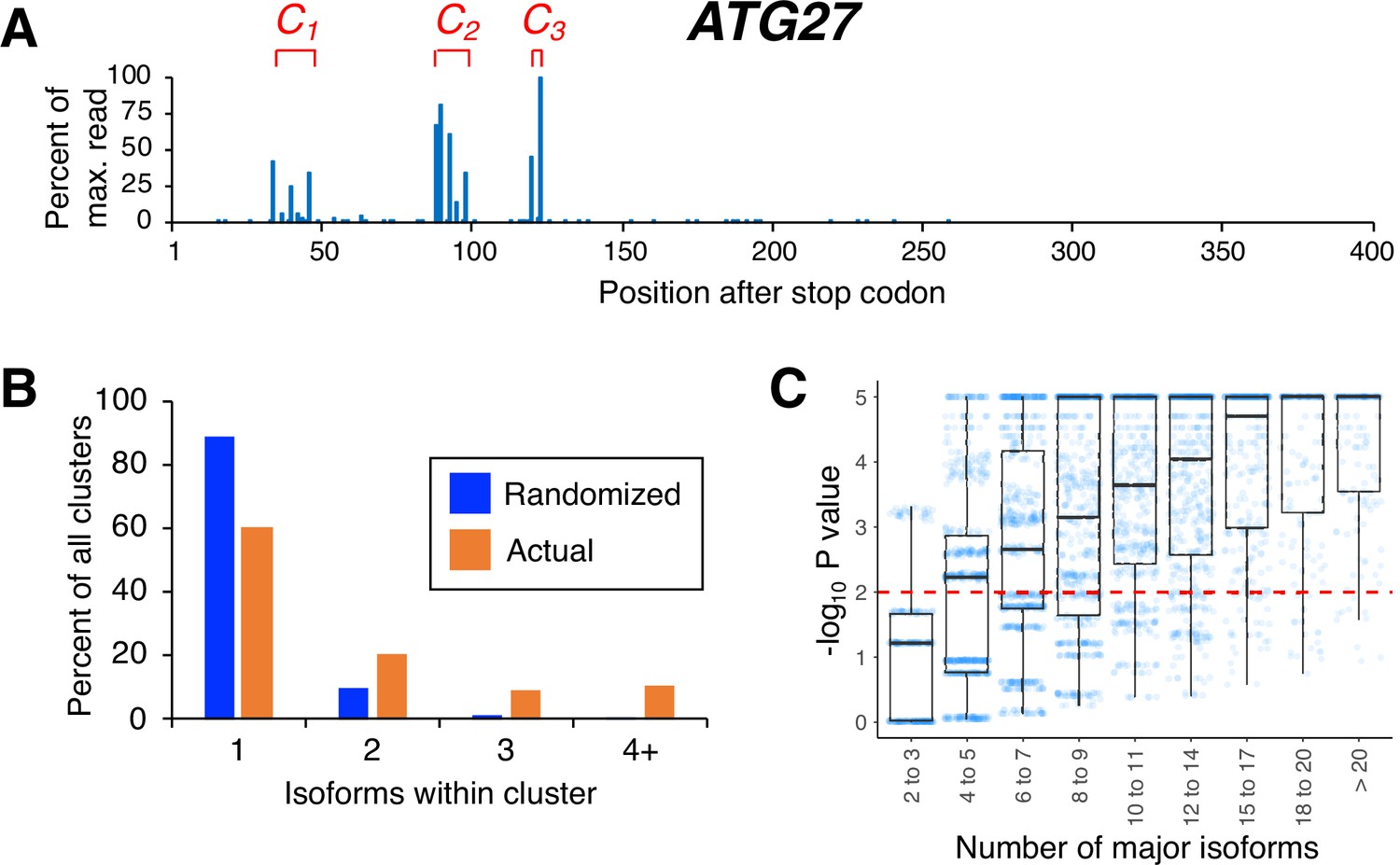
Isoforms in yeast 3’ untranslated regions (UTRs) are clustered.
(A) Polyadenylation profile of ATG27, a typical yeast gene, illustrating that major isoforms appear in clusters (represented as C1, C2, and C3 in red lettering). (B) Frequency distribution of clusters (all isoforms in cluster ≤4 nt apart) containing the indicated number of isoforms in either the randomized or genomic population. The number and frequency of all clusters were tabulated for 3774 genes (orange bars). Potential isoform positions were then shuffled 100,000 times within each gene’s 3’UTR, and the frequency and number of isoforms for each cluster were tabulated for every shuffled instance. Cluster frequencies were then combined across all 3774 genes and 100,000 shuffled instances/gene (blue bars). (C) Median likelihood (−log10 P value) that the experimentally observed cluster pattern for genes with the indicated number of major isoforms occurs by chance. Each point represents the probability that a given gene’s experimentally observed cluster frequency pattern is random. Horizontal bars inside boxplots represent the median values, while the top and bottom of each box represent the 25th and 75th percentiles. Values above dashed red line at –log10(P)=2 are considered statistically significant.
Figure 1—figure supplement 1
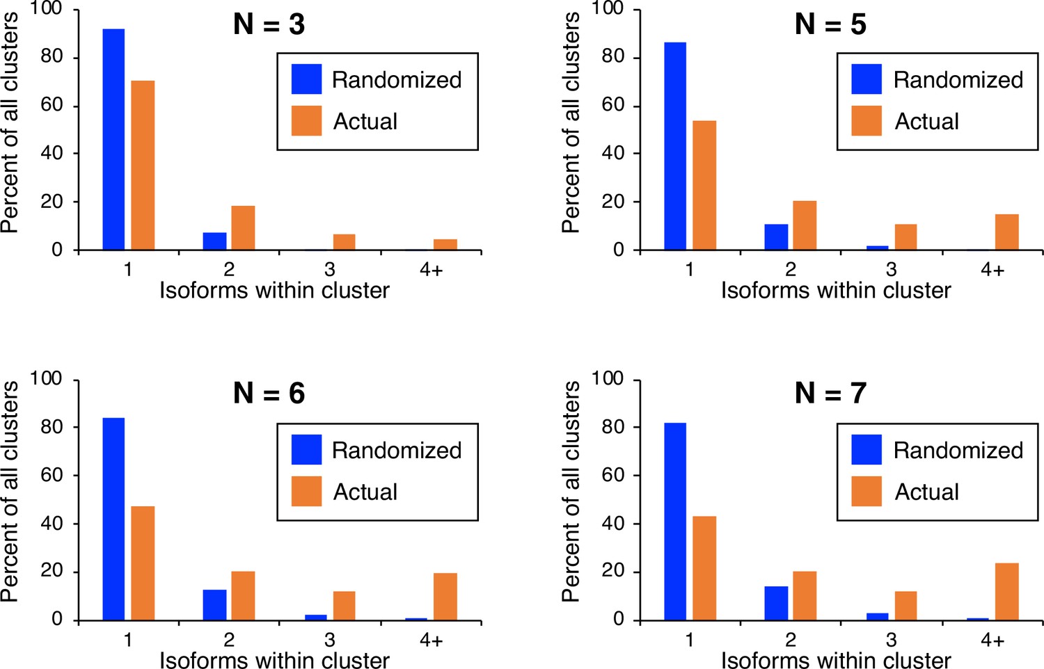
Frequency distributions of naturally occurring and randomized clusters as a function of different cluster definitions.
Cluster definition was altered to reflect either lower (n≤3; top left) or higher (n≤5, top right; n≤6, bottom left; n≤7, bottom right) maximal isoform spacing relative to the cluster definition used in Figure 1 (all isoforms in cluster ≤4 nt apart). The number and frequency of all clusters were tabulated for 3774 genes (orange bars). Potential isoform positions were then shuffled 100,000 times within each gene’s 3’ UTR, and the frequency and number of isoforms for each cluster were tabulated for every shuffled instance. Cluster frequencies were then combined across all 3774 genes and 100,000 shuffled instances/gene (blue bars).
Figure 1—figure supplement 2
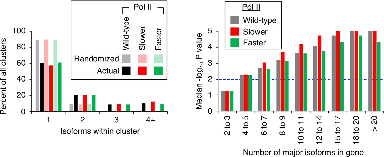
Pol II elongation rate does not affect isoform clustering in 3’ untranslated regions (UTRs).
(Left panel) Frequency distribution of clusters (all isoforms in cluster ≤4 nt apart) containing the indicated number of isoforms in either the randomized or genomic population. The number and frequency of all clusters were tabulated for 3774 genes in strains containing either wild-type (black bars), ‘slower’ (dark green bars), or ‘faster’ Pol II (dark red bars). In each strain, potential isoform positions were shuffled 100,000 times within each gene’s 3’ UTR, and the frequency and number of isoforms for each cluster were tabulated for every shuffled instance. Cluster frequencies were then combined across all 3774 genes and 100,000 shuffled instances/gene in each strain (wild-type: gray bars, ‘slower’: light red bars, ‘faster’: light green bars). (Right panel) Median likelihood (−log10 p value) that the experimentally observed cluster pattern for genes with the indicated number of major isoforms occurs by chance. Values above dashed black line at –log10(P)=2 are considered statistically significant.
Figure 2 with 1 supplement

Pol II elongation rate drives poly(A) cluster formation.
(A) Examples of poly(A) profiles in which ‘slower’/wild-type (WT) major isoform ratios (purple) decrease more rapidly within clusters than between clusters. Individual isoforms are defined by the number of nt downstream of the stop codon (x-axis). Clusters and inter-cluster regions are depicted as Cn and In in red and black lettering, respectively. The subscript n refers to the relative position of either the cluster or the inter-cluster region within the 3’ untranslated region, while brackets around clusters indicate that they contain <4 isoforms and thus were not used in cluster slope analysis. (B) Median relative ratios (downstream/upstream isoform) of genome-wide Rpb1(mutant)/Rpb1(WT) utilization at major isoform pairs as a function of nucleotide spacing either within clusters (circles) or in between clusters (diamonds). For each major isoform, Rpb1(mutant)/Rpb1(WT) utilization is computed by dividing the relative expression value of the isoform in the mutant strain by its relative expression in the WT strain. Relative ratios for each isoform pair are calculated by dividing downstream isoform utilization by upstream isoform utilization. Trend lines for ‘slower’/WT and ‘slow’/WT are depicted via dashes (within clusters) or as dots (between clusters).
Figure 2—figure supplement 1
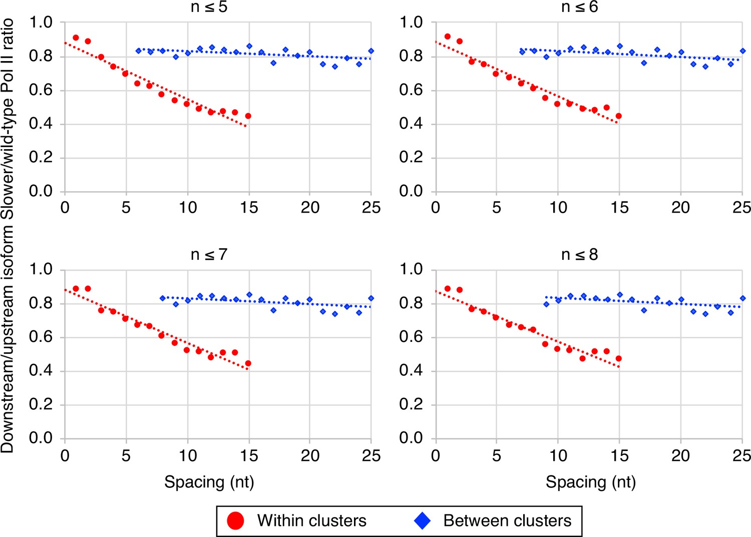
The link between Pol II elongation rate and poly(A) cluster formation is independent of exact cluster definition.
Median relative ratios (downstream/upstream isoform) of genome-wide ‘slower’/wild-type Pol II utilization at major isoform pairs as a function of nucleotide spacing either within clusters (circles) or in between clusters (diamonds). Maximal isoform spacing within clusters was varied between n≤5 and n≤8. For each major isoform, mutant/wild-type utilization is computed by dividing the relative expression value of the isoform in the mutant strain by its relative expression in the wild-type strain. Relative ratios for each isoform pair are calculated by dividing downstream isoform utilization by upstream isoform utilization.
Figure 3 with 1 supplement
Pol II elongation rate drives poly(A) cluster formation.
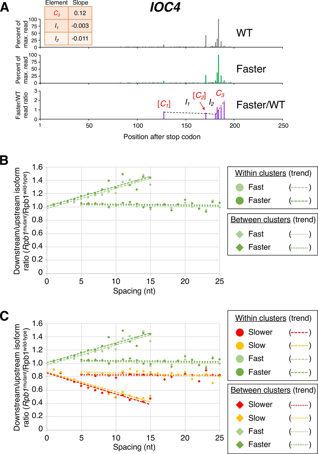
(A) Example poly(A) profile in which ‘faster’/wild-type (WT) major isoform ratios (purple) increase more rapidly within clusters than between clusters. Clusters and inter-cluster regions are depicted as Cn and In in red and black lettering, respectively. The subscript n refers to the relative position of either the cluster or the inter-cluster region within the 3’ untranslated region, while brackets around clusters indicate that they contain <4 isoforms and thus were not used in cluster slope analysis. (B) Median relative ratios (downstream/upstream isoform) of genome-wide Rpb1(mutant)/Rpb1(WT) utilization at major isoform pairs as a function of nucleotide spacing either within clusters (circles) or in between clusters (diamonds). For each major isoform, Rpb1(mutant)/Rpb1(WT) utilization is computed by dividing the relative expression value of the isoform in the mutant strain by its relative expression in the WT strain. Relative ratios for each isoform pair are calculated by dividing downstream isoform utilization by upstream isoform utilization. Trend lines for ‘faster’/WT and ‘fast’/WT are depicted via dashes (within clusters) or as dots (between clusters). (C) Median relative ratios (downstream/upstream isoform) of utilization at major isoform pairs as a function of nucleotide spacing in all four yeast elongation rate mutants (‘slower’/WT in red, ‘slow’/WT in yellow, ‘fast’/WT in light green, and ‘faster’/WT in dark green). Relative utilization ratios are depicted as either circles (within clusters) or diamonds (between clusters). Trend lines are dashed for within clusters and dotted between clusters.
Figure 3—figure supplement 1
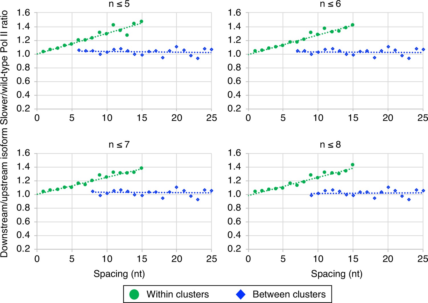
The link between Pol II elongation rate and poly(A) cluster formation is independent of exact cluster definition.
Median relative ratios (downstream/upstream isoform) of genome-wide ‘faster’/wild-type Pol II utilization at major isoform pairs as a function of nucleotide spacing either within clusters (circles) or in between clusters (diamonds). Maximal isoform spacing within clusters was varied between n≤5 and n≤8. For each major isoform, mutant/wild-type utilization is computed by dividing the relative expression value of the isoform in the mutant strain by its relative expression in the wild-type strain. Relative ratios for each isoform pair are calculated by dividing downstream isoform utilization by upstream isoform utilization.
Figure 4 with 2 supplements
Poly(A) cluster formation is also linked to Pol II elongation rate in human cell lines.
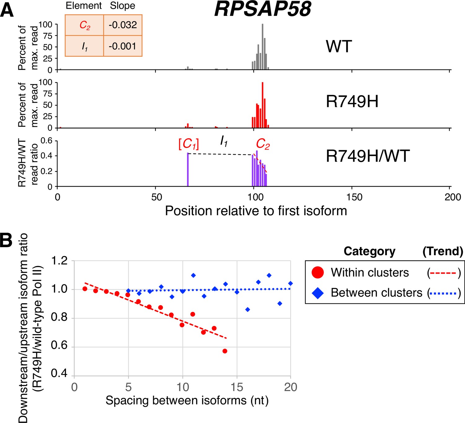
(A) An example of a poly(A) profile in which R749H/wild-type (WT) major isoform ratios (purple) decrease more rapidly within a cluster than between clusters. Clusters and inter-cluster regions are depicted as Cn and In in red and black lettering, respectively. The subscript n refers to the relative position of either the cluster or the inter-cluster region within the 3’ untranslated region while brackets around clusters indicate that they contain <4 isoforms and thus were not used in cluster slope analysis. (B) Median relative ratios (downstream/upstream isoform) of isoform utilization (R749H/WT Pol II) in human 3’ isoform pairs as a function of nucleotide spacing. Relative ratios are depicted either as circles (within clusters) or as diamonds (between clusters), while trend lines are either dashed (within clusters) or dotted (between clusters).
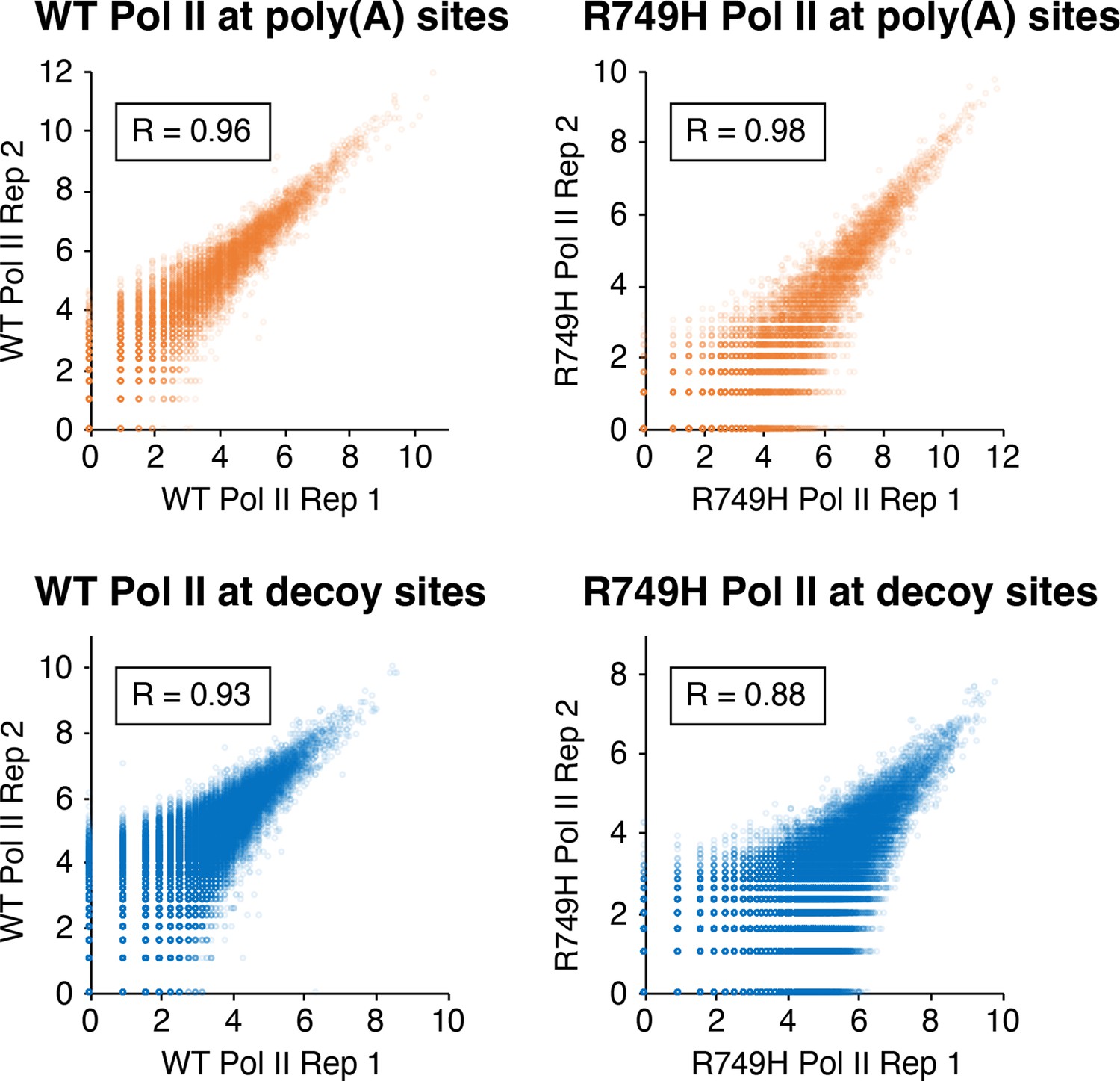
Figure 4—figure supplement 1
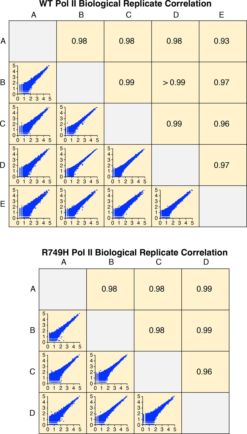
Correlation of wild-type (WT) or R749H Pol II biological replicates.
Axes in bottom left panels represent log10 of isoform reads. Each pairwise comparison panel contains >49,000 (WT) or >32,000 (R749H) isoforms with non-zero reads in both replicates. Upper right panels indicate the Pearson R value of each comparison.
Figure 4—figure supplement 2
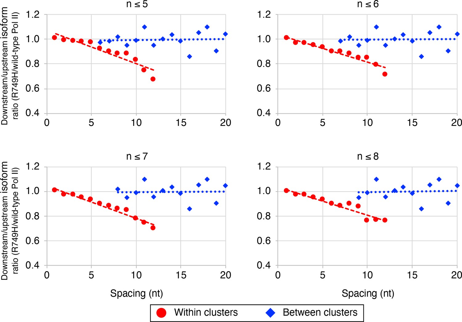
The link between Pol II elongation rate and poly(A) cluster formation is independent of the exact cluster definition in mammalian cells.
Median relative ratios (downstream/upstream isoform) of genome-wide R749H/wild-type (WT) Pol II utilization at major isoform pairs as a function of nucleotide spacing either within clusters (circles) or between clusters (diamonds). Maximal isoform spacing within clusters was varied between 5 and 8. For each major isoform, R749H/WT utilization is computed by dividing the relative expression value of the isoform in the R749H cell line by its relative expression in the WT cell line. Relative ratios for each isoform pair are calculated by dividing downstream isoform utilization by upstream isoform utilization.
Figure 5
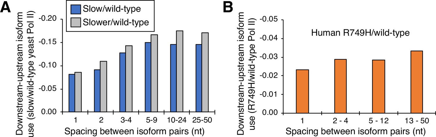
Cluster-independent link between Pol II elongation rate and poly(A) formation.
(A) Median utilization difference (downstream isoform mutant/wild-type expression ratio minus upstream isoform mutant/wild-type expression ratio) is plotted for either ‘slower’/wild-type (gray bars) or ‘slow’/wild-type (blue bars) as a function of isoform spacing. (B) Median utilization difference (downstream isoform R749H/wild-type expression ratio minus upstream isoform R749H/wild-type expression ratio) as a function of isoform spacing.
Figure 6

GC-rich region just downstream of isoform clusters.
(A) GC content in a region downstream of clusters is correlated to cluster slopes in ‘slow’/wild-type (upper left), ‘slower’/wild-type (bottom left), ‘fast’/wild-type (top left), and ‘faster’/wild-type (bottom left) datasets. Pearson R at each position (blue; left axes) represents the correlation of GC content and cluster slopes in a 10-nt window starting at the position indicated on the x-axis. Red lines (right axes) represent false discovery rate (FDR)-corrected –log10 P values of each correlation, the dashed red line is the significance cutoff (correlations above it are deemed significant), and significant regions are highlighted in gray boxes. Segments at the bottom of each graph indicate the span of the GC-enriched sequence in each mutant/wild-type Pol II dataset. (B) GC content at +13 to +30 is linked to cluster slopes. Cluster slopes for ‘slower’/wild-type, ‘slow’/wild-type, ‘fast’/wild-type, and ‘faster’/wild-type were individually separated into quintiles, with the most negatively sloped clusters depicted on the left and the most positively sloped clusters depicted on the right. For each cluster, the percent change in GC content at +13 to +30 was computed relative to the median GC content at the equivalent genomic coordinates within 3’ untranslated regions. The y-axis depicts the average percent change in GC content for all clusters of a given category within each quintile. Median slopes for cluster categories within each quintile are shown on the bottom. (C) GC-rich region immediately downstream of poly(A) clusters in yeast. Elongating Pol II makes numerous contacts (black circles: identical residues in both mammalian and yeast Rpb1; gray circles: conserved residues in both mammalian and yeast Rpb1) with both DNA strands (purple: template strand, blue: non-template strand) and nascent RNA (red). The RNA addition site (+1), Pol II-protected region (gray oval), RNA:DNA hybrid (yellow), and the +13 to +30 region (boxed) are shown. Adapted from Bernecky et al., 2016.
Figure 7 with 1 supplement

Pol II occupancy and AT composition at either READS poly(A) or decoy intronic AATAAA sites in human HEK293 cell lines harboring either wild-type (‘WT’) or slow (‘R749H’) Pol II variants.
(A) eNETseq signal for WT (black; right axis) and R749H (red; right axis) at 2989 READS poly(A) sites (≥20 reads/site in both WT and R749H). Percent AT composition is in blue with the scale on the left axis. The two-sided vertical arrow indicates the difference between the Pol II signal at the region 40-100 nt downstream of the poly(A) site and the average Pol II signal (dashed lines). (B) eNETseq signal for WT (black; right axis) and R749H (red; right axis) at 15,865 decoy intronic AATAAA sites (≥10 reads/site in both WT and R749H). Percent AT composition is in blue, with the scale on the left axis. The dashed line indicates the average Pol II signal; note that Pol II occupancy does not increase downstreams of the intronic AATAAA sites.
Figure 7—figure supplement 1
Correlation of eNETseq biological replicates at poly(A) and decoy intronic AATAAA sites.
For the wild-type Pol II (‘WT’; left panels) and R749H (right panels) cell lines, the log2 of the total number of eNETseq reads at each site ±100 nt is plotted for each replicate. Pearson correlation values for each comparison are depicted in boxes.
Figure 8
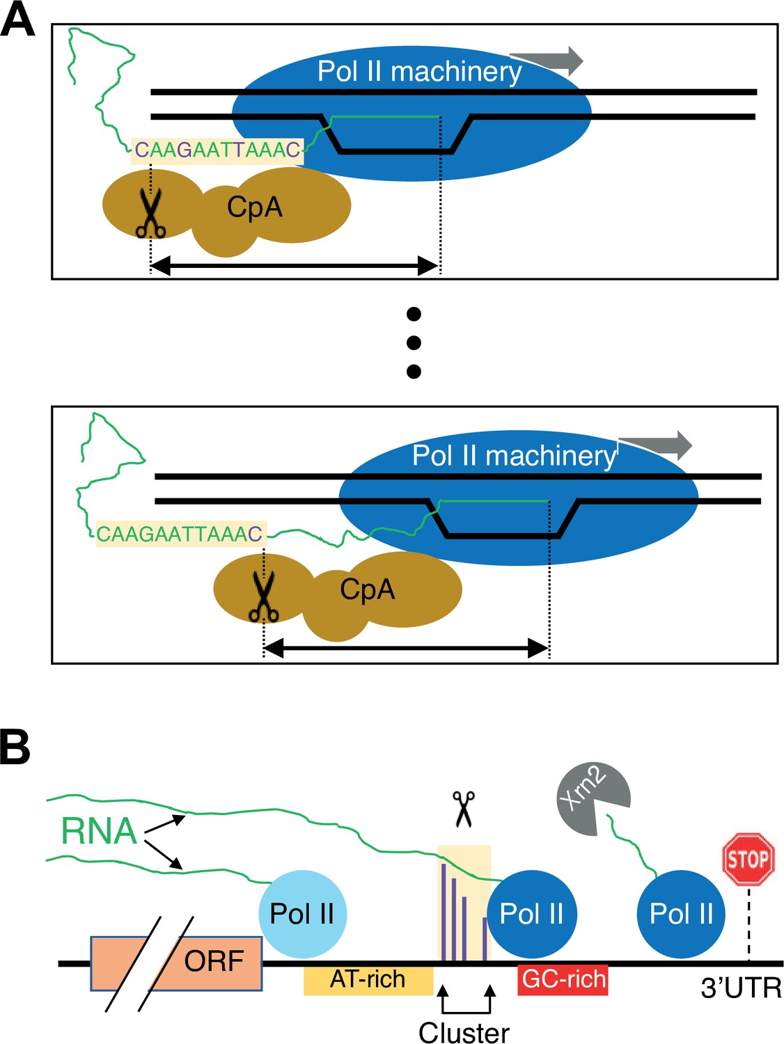
Schematic of the link between Pol II elongation rate and poly(A) formation.
(A) Nucleotide-level link between Pol II elongation and cleavage/polyadenylation (CpA). As the Pol II machinery (dark blue) elongates the nascent RNA one nucleotide at a time, upstream sequences of the newly synthesized RNA strand become exposed, leading the CpA complex (gold) to cleave and polyadenylate the nascent RNA at preferred residues (purple). The Pol II and CpA machineries are spatially, and likely physically, coupled so that cleavage occurs at a constrained distance from the position of the active site of elongating Pol II (black arrow). (B) Gene-level view of CpA. Rapidly elongating Pol II (light blue) traverses the gene body and 3’ untranslated region (UTR) until it encounters an AT-rich region (gold) and/or a GC-rich stretch downstream of clusters (red), which cause it to slow down (dark blue). The nascent RNA (green) extruded out of the slowing elongating Pol II complex gets cleaved and polyadenylated (scissors) at one of the preferred positions within the cluster (purple). The Pol II complex then continues to elongate a short and unstable non-coding RNA that is endonucleolytically degraded by Xrn2 (gray) and eventually terminates at a downstream position (stop sign).
Additional files
-
Supplementary file 1
Supplemental file showing all clusters in YPD.
- https://cdn.elifesciences.org/articles/83153/elife-83153-supp1-v2.xlsx
-
MDAR checklist
- https://cdn.elifesciences.org/articles/83153/elife-83153-mdarchecklist1-v2.docx
Download links
A two-part list of links to download the article, or parts of the article, in various formats.
Downloads (link to download the article as PDF)
Open citations (links to open the citations from this article in various online reference manager services)
Cite this article (links to download the citations from this article in formats compatible with various reference manager tools)
Nucleotide-level linkage of transcriptional elongation and polyadenylation
eLife 11:e83153.
https://doi.org/10.7554/eLife.83153


