Clarifying the role of an unavailable distractor in human multiattribute choice
- Department of Neurophysiology and Pathophysiology, University Medical Center Hamburg-Eppendorf, Germany
- School of Psychological Science, University of Bristol, United Kingdom
Figures
Figure 1
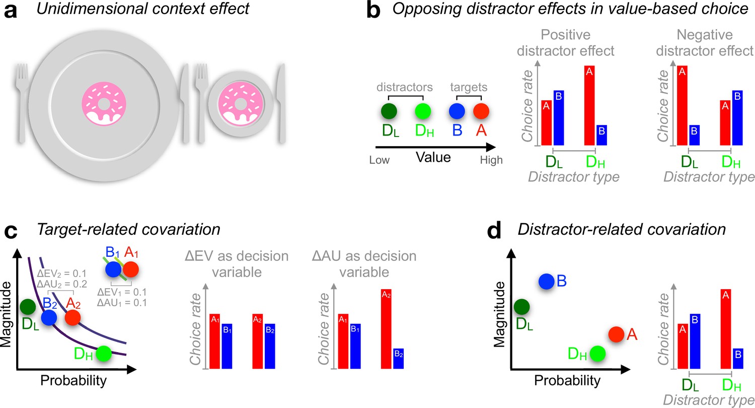
Context effects in decision-making.
(a) Judgement about object size can be influenced by the surround. (b) Documented positive (Chau et al., 2014) or negative (Louie et al., 2013) distractor effects occur at the level of unidimensional value. A higher-valued distractor (DH), compared with a lower-valued distractor (DL), can increase the choice rate of A relative to B (positive distractor effect) but can also decrease the choice rate of A relative to B (negative distractor effect), leading to opposing distractor effects in past reports (Chau et al., 2014; Louie et al., 2013). (c) During risky choices, if people derive subjective utilities of prospects by integrating reward magnitude and probability additively (additive utility or AU), and if targets {A2, B2} are more frequently paired with distractor DH while targets {A1, B1} with DL, then a positive distractor effect could be explained by additive integration (because ΔAU1 < ΔAU2) rather than the distractor’s expected value (EV: magnitude × probability). Curves: EV indifference lines. (d) Similarly, relative preference changes for target alternatives A and B can be driven by an attraction-effect bias (Huber et al., 1982; Dumbalska et al., 2020) that depends on the position of the decoy D with respect to each target alternative. If DH appears more often closer to A while DL being more often closer to B, a positive distractor effect will ensue as a by-product of the attraction effect. In all illustrations, A-alternatives are always better than B-alternatives, with D-alternatives denoting the distractor (decoy) alternatives.
Figure 2 with 3 supplements
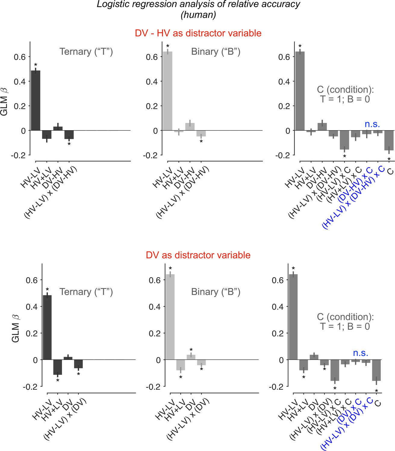
Re-assessing distractor effects beyond target-related covariations in ternary- and binary-choice trials.
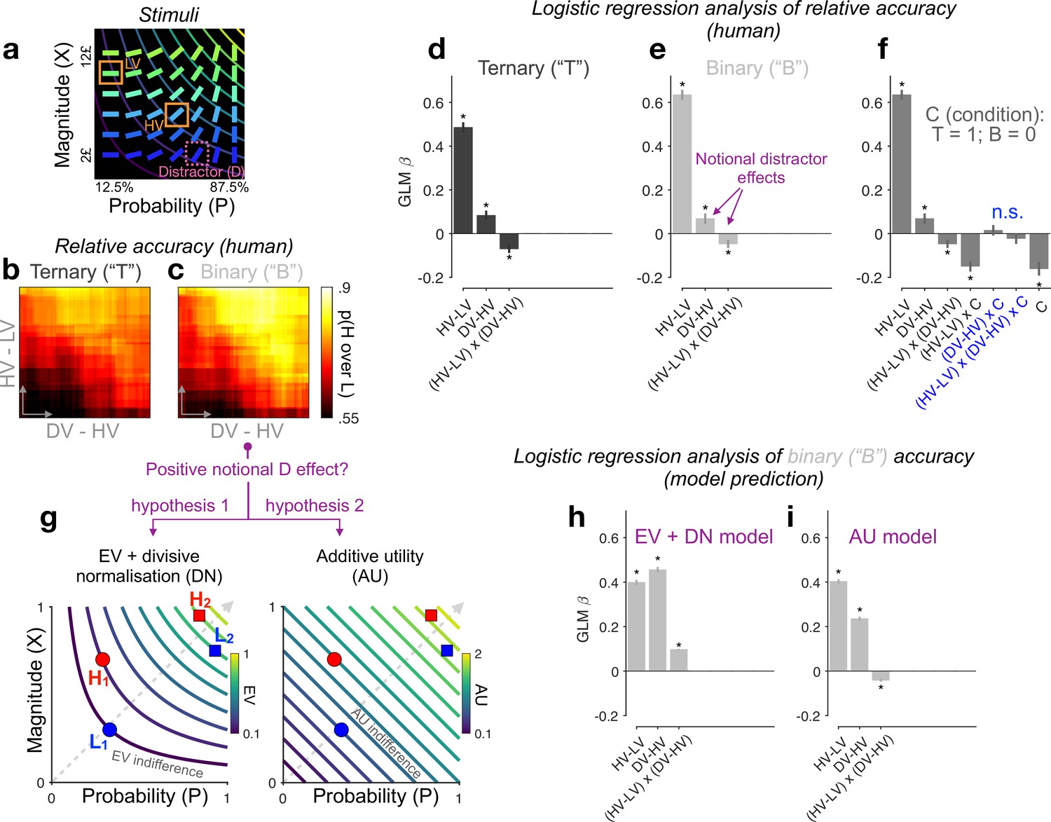
(a) Multiattribute stimuli in a previous study (Chau et al., 2014). Participants made a speeded choice between two available options (HV: high expected value; LV: low expected value) in the presence (ternary) or absence (binary) of a third distractor option (‘D’). Three example stimuli are labelled for illustration purposes only. In the experiment, D was surrounded by a purple square to show that it should not be chosen. (b, c) Relative choice accuracy (probability of H choice among all H and L choices) in ternary trials (panel b) and in binary-choice baselines (panel c) plotted as a function of both the expected value (EV) difference between the two available options (HV − LV) (y-axis) and the EV difference between D and H (x-axis). Relative choice accuracy increases when HV − LV increases (bottom to top) as well as when DV − HV increases (left to right, i.e., positive D effect). (d–f) Predicting relative accuracy in human data using regression models (Methods). Asterisks: significant effects [p < 0.05; two-sided one-sample t-tests of generalised linear model (GLM) coefficients against 0] following Holm’s sequential Bonferroni correction for multiple comparisons. n.s.: non-significant. (g) Rival hypotheses underlying the positive notional distractor effect on binary-choice accuracy. Left: EV indifference contour map; Right: additive utility (AU) indifference contour map. Utility remains constant across all points on the same indifference curve and increases across different curves in evenly spaced steps along the direction of the dashed grey line. Decision accuracy scales with Δ(utility) between H and L in binary choices. Left (hypothesis 1): Δ(EV) = (HV − LV)/(HV + LV) by virtue of divisive normalisation (DN); because HV2 − LV2 = HV1 − LV1, and HV2 + LV2 > HV1 + LV1, Δ(EV2) becomes smaller than Δ(EV1). Right (hypothesis 2): Δ(AU) = AUH − AUL; Δ(AU2) < Δ(AU1) by virtue of additive integration. (h, i) Regression analysis of model-predicted accuracy in binary choice. EV + DN model corresponds to hypothesis 1 whilst AU model corresponds to hypothesis 2 in panel g. Error bars = ± standard error of the mean (SEM) (N = 144 participants).
Figure 2—figure supplement 1
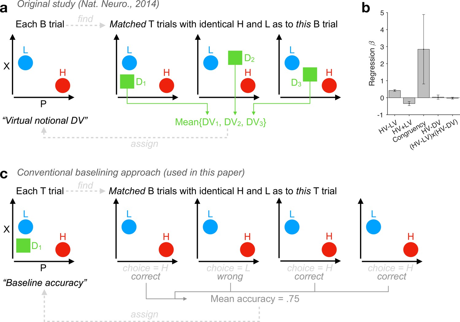
Distinctions between our baselining approach and the method in the original study (Chau et al., 2014).
(a) Method in the original study (Chau et al., 2014): A schematic showing that the mean DV across relevant ternary trials (‘T’) is taken as a notional DV for each individual binary trial (‘B’). For each participant, among the 150 T trials there are 149 unique T conditions with a specific combination of P and X attributes across the 3 alternatives, while among the 150 B trials there are only 95 unique B conditions with a specific combination of P and X across the 2 options. The T and B trials do not have one-to-one mapping even if the unique stimulus positions (among four quadrants of the screen) are taken into consideration. (b) A successful reproduction of an invalid control analysis in the Supplementary file 3b of the original study (Chau et al., 2014): ‘The effect of HV-D on human behavior was specific to distractor trials’ using the notional DV depicted in panel a. Error bars: ± standard error of the mean (SEM) across participants (N = 21). (c) Our baselining approach uses a new dependent variable, the trial-by-trial baseline accuracy, via identifying all matched B trials (number of trials 1 ≤ nB ≤ 6) of every T trial. Of note, when analysing choice accuracies in B trials using logistic regression (e.g., Figure 2), Matlab’s glmfit takes a two-column response matrix whose first column indicates the number of correct responses (H choices) for each observation and second column indicates nB for each observation.
Figure 2—figure supplement 2
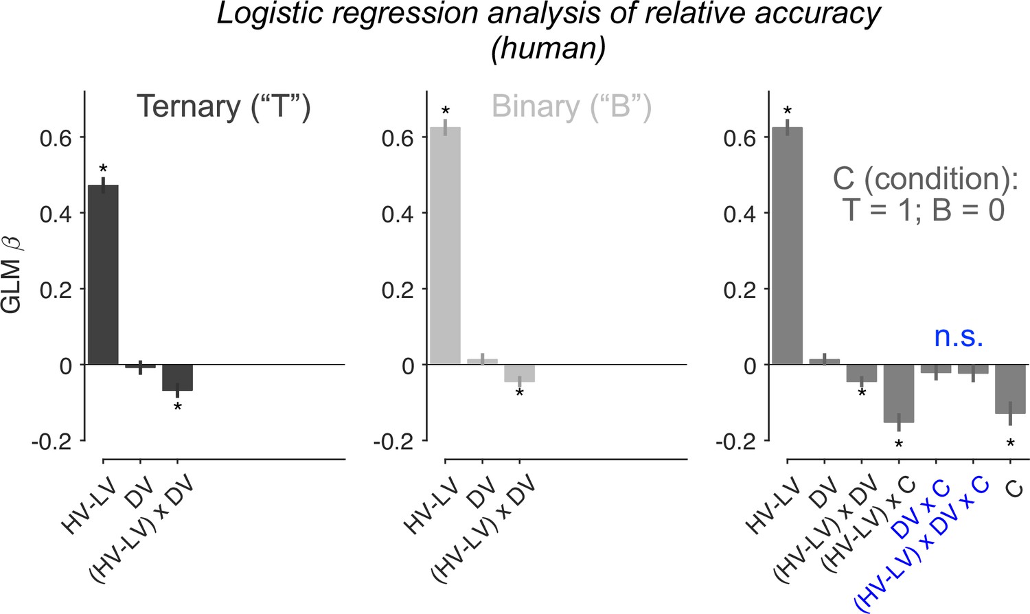
Re-assessing distractor effects beyond target-related covariations.
Figure 2—figure supplement 3
Re-assessing distractor effects beyond target-related covariations.
The generalised linear models (GLMs) here included an additional regressor HV + LV. Error bars = ± standard error of the mean (SEM) (N = 144 participants). Asterisks: significant effects (p < 0.05; two-sided one-sample t-tests of GLM beta coefficients against 0) following Holm’s sequential Bonferroni correction for multiple comparisons. n.s.: non-significant.
Figure 3 with 1 supplement
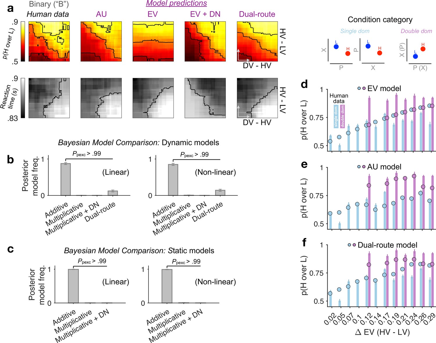
Modelling binary-choice behaviour.
(a) Human vs. model-predicted choice accuracy and reaction time (RT) patterns. (b, c) Bayesian model comparison based on cross-validated log-likelihood. Linear and non-linear: different psychometric transduction functions for reward magnitude and probability (see Methods). Linear multiplicative: EV; linear additive: AU. Dynamic model: optimisation based on a joint likelihood of choice probability and RT; Static model: optimisation based on binomial likelihood of choice probability. (d–f) Model predictions (circles) plotted against human data (bars) for different condition categories [H dominates L on one attribute only, that is, single dom. (81% of all trials), or on both attributes, that is, double dom. (only 19%)] at each level of HV – LV. Error bars = ± standard error of the mean (SEM) (N = 144 participants).
Figure 3—figure supplement 1
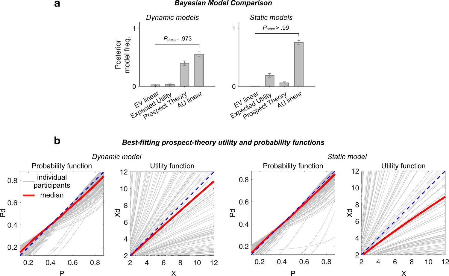
Additional multiplicative models (expected utility and prospect theory).
(a) Bayesian random-effect comparison of models fit to binary-choice trials. (b) Visualisation of best-fitting utility and probability functions of the prospect-theory model. Grey curves: individual participants’ best-fitting functions; red curves: median across participants (N = 144). The typical best-fitting probability function tends to overweigh low probabilities and the typical utility function (distorted magnitude) tends to be concave (i.e., compressive non-linearity).
Figure 4 with 1 supplement

Multiattribute context effects.
(a) The attraction effect (Huber et al., 1982) can happen when D is close to and dominated by H or L. The repulsion effect (Dumbalska et al., 2020) can happen when D is close to but dominates H or L. (b) T − B p(H over L) plotted as a function of D’s relative Euclidean distance to H vs. L in the attribute space and D’s additive utility (AU) dominance—‘superior’ (‘inferior’) D lies on a higher (lower) AU indifference line than both H and L. Error bars: ± standard error of the mean (SEM) across participants (N = 144). (c) Condition-unspecific bias of p(H over L) in ternary conditions relative to binary conditions. (d) Bias-corrected T − B p(H over L). Black asterisks: significant context effects (Bonferroni–Holm corrected p < 0.05; two-tailed one-sample t-tests against 0). (e) Bias-corrected T − B p(H over L) predicted by different models. Grey asterisks: significant difference between model predictions and human data (uncorrected p < 0.05; two-tailed paired-sample t-tests). (f) Main effect of D’s AU dominance (superior vs. inferior) on T − B relative accuracy change in human data and model predictions. (g) Bayesian model comparison of context-dependent models (also see Figure 4—figure supplement 1). (h) Model recovery (Methods). Text in each cell: posterior model frequency; Heatmap: protected exceedance probability (Ppexc) that a fitted model (each column) has the highest log-likelihood given input ternary-trial data (choice probabilities and RTs) simulated by a certain model (each row).
Figure 4—figure supplement 1
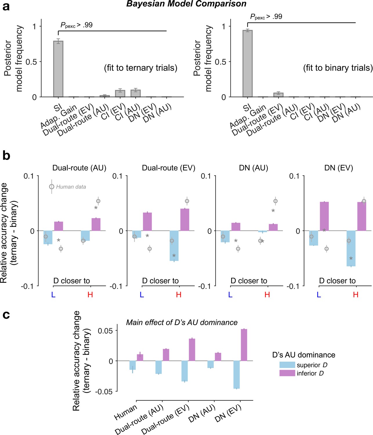
Additional modelling results.
(a) Bayesian random-effects model comparison based on cross-validated log-likelihood (fivefolds). SI: selective integration model; Adap. Gain: adaptive gain model; CI: context independent; EV: expected value; AU: additive utility. Dual-route and divisive normalisation (DN) model predictions for the relative accuracy change (Ternary minus Binary, T − B) as a function of (b) both D’s AU dominance (colour of the bars) and D’s position similarity to H and L in the 2D attribute space, or (c) D’s AU dominance only (main effect). AU: additive utility; EV: expected value. Error bars: ± standard error of the mean (SEM) across participants (N = 144).
Figure 5 with 1 supplement
Selective gating, context effects, and decision noise.
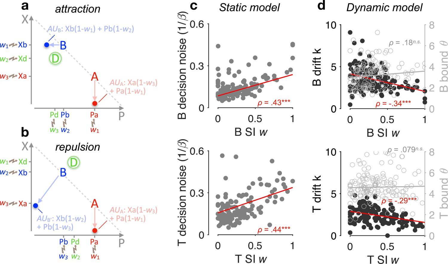
(a, b) By virtue of selective integration (SI), alternatives A, B, and D are ranked within each attribute dimension; SI weights are then assigned to the sorted alternatives accordingly (for illustration, w1 = 0, w2 = 0.5, and w3 = 0.9). Attribute values are selectively suppressed in proportion to the SI weights, that is, lower ranked values are suppressed more strongly. As a result of SI (assuming any w1 < w2 ≤ w3), the additive utility (AU) of B is higher in the case of panel a than the AU of B′ in the case of panel b due to the distinct locations of decoy D. (c) Relationship between SI w and decision noise. Red lines: robust linear regression fits (using Matlab’s robustfit). : softmax inverse temperature. Top: binary trials (‘B’); bottom: ternary trials ('T’) (ternary SI w: mean across w2 and w3); SI w = 0: lossless integration, that is, attributes maintain their original values; SI w > 0: selective integration; SI w = 1: losing attribute value shrinks to 0. ρ: Spearman’s rank correlation coefficient. ***p < 0.0001. (d) Relationship between SI w and drift sensitivity k (filled black) or decision bound (open grey). Each point represents a participant (N = 144 in total).
Figure 5—figure supplement 1
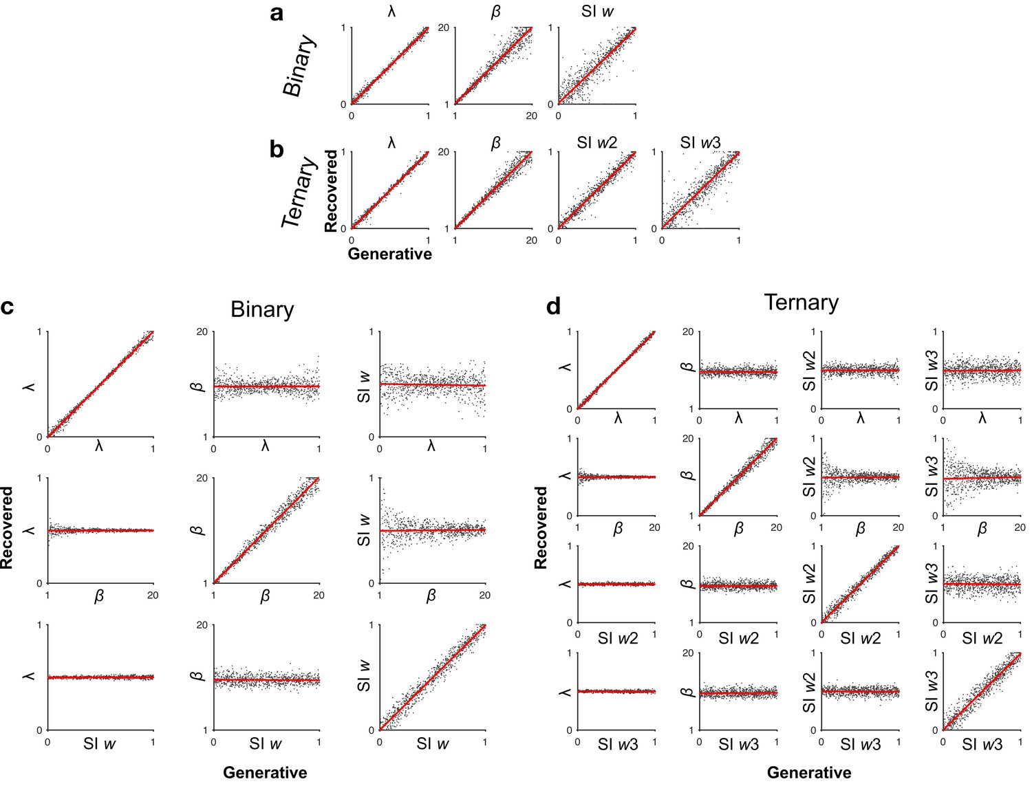
Parameter recovery.
(a, b) Recovery of selective integration (SI) model parameters by simulating choice probabilities (1000 trials) based on a grid of uniformly distributed parameter values (n = 800 each) and then estimating the best-fitting parameters. (c, d) Each row shows a case of simulating choice probabilities by varying 1 model parameter while fixing all other parameters ( = 0.5, = 10, SI w = 0.5) and then estimating the best-fitting parameter values via model fitting. On-diagonal panels show the recovery of each parameter as a function of itself (all |Pearson’s r| > 0.99), whilst off-diagonal panels suggest that variation in irrelevant parameters do not bias the recovery of any given parameter of interest (all |Pearson’s r| < 0.056, p > 0.1).
Additional files
-
Supplementary file 1
Optimal parameter estimates of dynamic models: mean (SE) and cross-validated log-likelihood (CV LL).
- https://cdn.elifesciences.org/articles/83316/elife-83316-supp1-v2.docx
-
Supplementary file 2
Optimal parameter estimates of static models: mean (SE) and cross-validated log-likelihood (CV LL).
- https://cdn.elifesciences.org/articles/83316/elife-83316-supp2-v2.docx
-
Supplementary file 3
Generalised linear models (GLMs) using subjective additive utility (AU) regressors.
*Significant effects (p < 0.05; two-sided one-sample t-tests of GLM coefficients against 0) following Holm’s sequential Bonferroni correction for multiple comparisons. C: ‘Condition’ (binary vs. ternary).
- https://cdn.elifesciences.org/articles/83316/elife-83316-supp3-v2.docx
-
Supplementary file 4
Optimal parameter estimates of context-dependent dynamic models: mean (SE) and cross-validated log-likelihood (CV LL).
- https://cdn.elifesciences.org/articles/83316/elife-83316-supp4-v2.docx
-
MDAR checklist
- https://cdn.elifesciences.org/articles/83316/elife-83316-mdarchecklist1-v2.docx
Download links
A two-part list of links to download the article, or parts of the article, in various formats.
Downloads (link to download the article as PDF)
Open citations (links to open the citations from this article in various online reference manager services)
Cite this article (links to download the citations from this article in formats compatible with various reference manager tools)
Clarifying the role of an unavailable distractor in human multiattribute choice
eLife 11:e83316.
https://doi.org/10.7554/eLife.83316


