High-resolution volumetric imaging constrains compartmental models to explore synaptic integration and temporal processing by cochlear nucleus globular bushy cells
- Department of Medical Engineering, University of South Florida, United States
- Department of Otolaryngology, Head and Neck Surgery, West Virginia University, United States
- Department of Neurosciences, University of California, San Diego, United States
- National Center for Microscopy and Imaging Research,University of California, San Diego, United States
- Department of Otolaryngology/Head and Neck Surgery, University of North Carolina at Chapel Hill, United States
- Department of Cell Biology and Physiology, University of North Carolina, United States
Figures
Figure 1 with 2 supplements
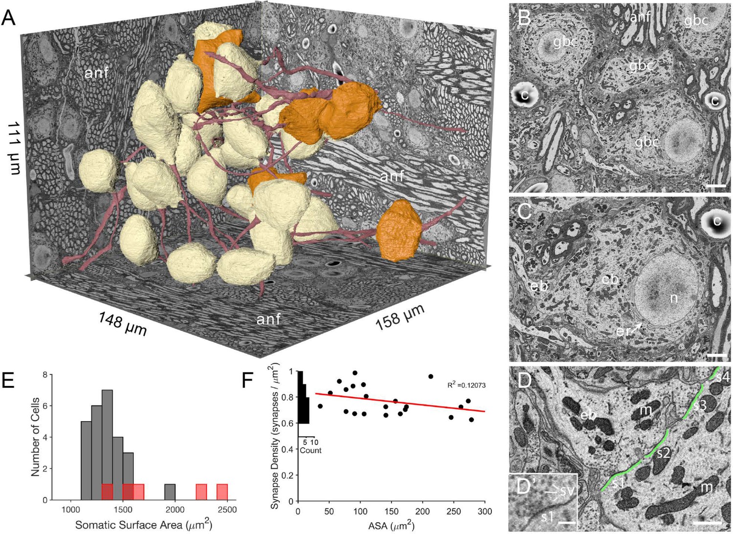
The imaged volume in the cochlear nucleus captures globular bushy (GBC) and multipolar cells (MC), and reveals synaptic sites.
(A) The VCN region that was imaged using SBEM is depicted within walls of the image volume. Twenty-six GBCs (beige) and 5 MCs (orange) are shown with their axons (red). Left rear wall transects auditory nerve (anf) fascicles, which run parallel to the right rear wall and floor. Non-anf axons exit into the right rear wall and floor as part of other fascicles that are cross-sectioned. The complete volume can be viewed at low resolution in Figure 1—video 1. (B) Example image, cropped from the full field of view, from the data set in panel A. Field of four GBC (gbc) cell bodies, myelinated axons in anf fiber fascicles, and capillaries (c). (C) Closeup of the cell body (cb) of lower right GBC from panel B, illustrating the eccentrically located nucleus (n), short stacks of endoplasmic reticulum (er) aligned with the cytoplasm-facing side of the nuclear envelope, and contact by an endbulb (eb). (D) Closeup of the labeled endbulb contacting the cell in panel C (eb), revealing its initial expansion along the cell surface. Apposed pre- and postsynaptic surface area (ASA; green) are accurately determined by excluding regions with intercellular space (ASA is discontinuous), and synaptic sites (s1-4) are indicated as clusters of vesicles with some contacting the presynaptic membrane. (D’) Inset in panel D is closeup of synapse at lower left in panel D. It shows defining features of synapses in these SBEM images, which include clustering of vesicles near the presynaptic membrane, convex shape of the postsynaptic membrane, and in many cases a narrow band of electron-dense material just under the membrane, as evident here between the ‘s1’ symbol and the postsynaptic membrane.Green line indicates regions of directly apposed pre- and postsynaptic membrane, and how this metric can be accurately quantified using EM. (E) Histogram of all somatic surface areas generated from computational meshes of the segmentation. GBCs are denoted with grey bars and MCs with red bars. (F) Synapse density plotted against ASA shows a weak negative correlation. Marginal histogram of density values is plotted along the ordinate. Scale bars = 5 μm in B, 2 μm in C, 1 μm in D, 250 nm in D’.
Figure 1—figure supplement 1
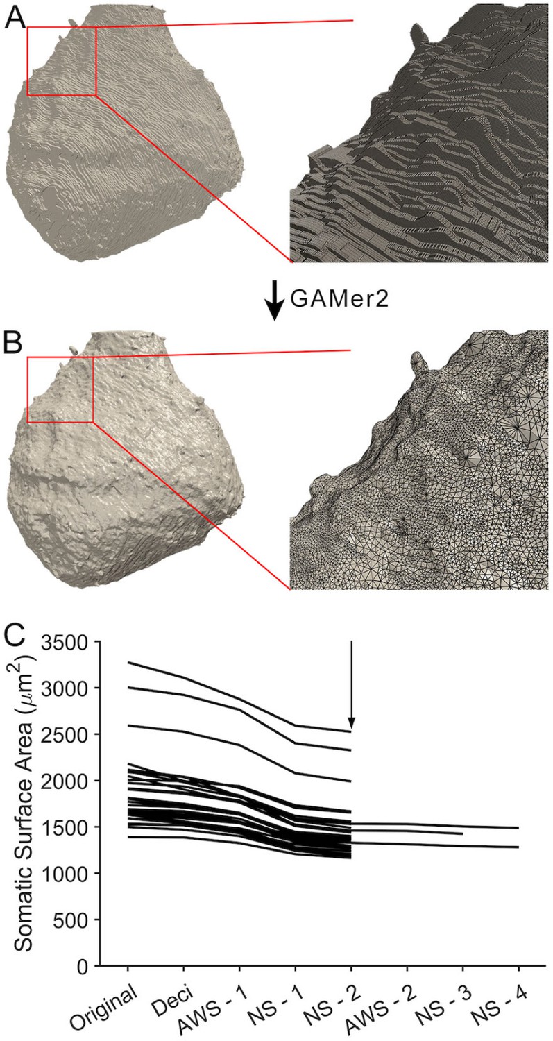
Steps in mesh generation and compartmental representation from EM volumes, related to Figure 1A.
(A) Cell membranes of objects (cell body of a bushy cell in this case) were traced and assembled into stacks. Each tissue section appears as a slab, seen clearly in expanded view at right. The slab thickness is the 60nm section thickness used during imaging. (B) The GAMer2 algorithm (Lee et al., 2020b) was used to create a mesh surface enclosing the volume, comprised of isosceles triangles, that preserved real surface irregularities such as small protrusions. (C) Decimation and smoothing algorithms were successively applied until the meshed surface area reached an asymptote (vertical arrow). The change in area for all reconstructed somas are shown. After testing multiple cycles on three cells, values at NS-2 stage (see Materials and methods) were used for all cells.
Figure 1—video 1
Exploration of the relation between an image volume and a globular bushy cell (GBC) mesh derived from that volume.
This video opens with a top-down view of the SBEM image volume from the ventral cochlear nucleus. The video zooms in as the volume is slowly cut away to reveal GBC05, including its dendrites (red), cell body (beige), axon (pink), and all large somatic inputs (various colors). The perspective then shifts laterally to view several of the large terminals (various colors) contacting the cell body.
Figure 2 with 4 supplements
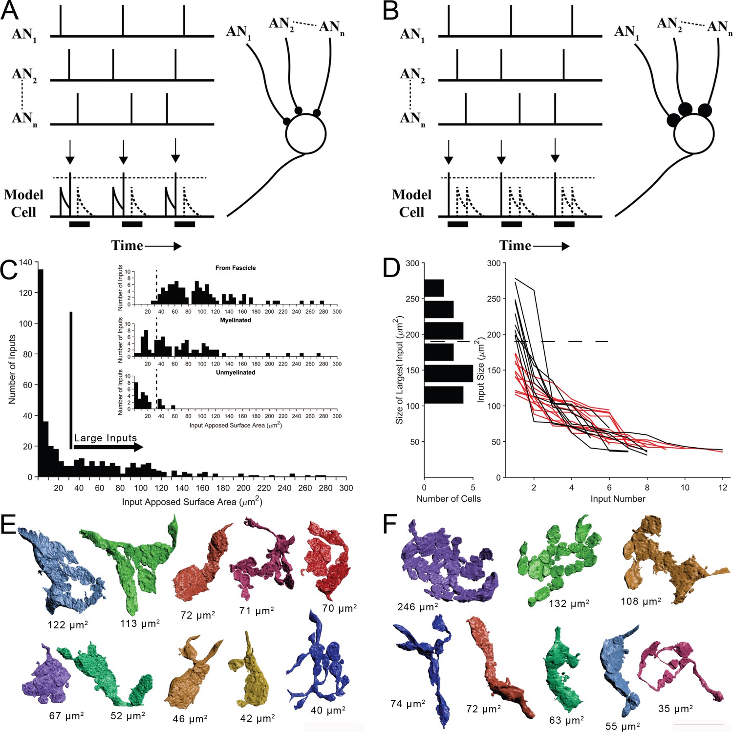
Two competing models for synaptic convergence evaluated using size profiles of endbulb terminals.
(A) Coincidence Detection model, all inputs are subthreshold (small circles), have similar weight, and at least two inputs are active in a short temporal window to drive a postsynaptic spike. Each vertical bar is a presynaptic spike and each row is a separate auditory nerve (AN) input. Bottom line is activity of postsynaptic globular bushy cell (GBC). EPSPs are solid; action potentials indicated by vertical arrows. Dotted lines are inputs that occur during the refractory period (solid bar). Drawn after Joris et al., 1994a. (B) First-Latency model, whereby all inputs are suprathreshold (large circles), have similar weight, and the shortest latency input drives a postsynaptic spike. Longer latency inputs are suppressed during the refractory period. For a periodic sound, both models yield improved phase-locking in the postsynaptic cell relative to their auditory nerve (AN) inputs. (C) Histogram of input sizes, measured by apposed surface area (ASA), onto GBC somata. Minimum in histogram (vertical bar) used to define large somatic inputs (arrow). Inset: Top. Size distribution of somatic terminals traced to auditory nerve fibers within the image volume. Middle. Size distribution of somatic terminals with myelinated axons that exited the volume without being traced to parent fibers within volume. Bottom. Size distribution of somatic terminals with unmyelinated axons. Some of these axons may become myelinated outside of the image volume. Small terminals (left of vertical dashed lines) form a subset of all small terminals across a population of 15 GBCs. See Figure 2—figure supplement 1 for correlations between ASA and soma areas. (D) Plot of ASAs for all inputs to each cell, linked by lines and ranked from largest to smallest. Size of largest input onto each cell projected as a histogram onto the ordinate. Dotted line indicates a minimum separating two populations of GBCs. Linked ASAs for GBCs above this minimum are colored black; linked ASAs for GBCs below this minimum are colored red. (E, F). All large inputs for two representative cells. View is from postsynaptic cell. (E) The largest input is below threshold defined in panel (D). See Figure 2—figure supplement 2 for all 12 cells with this input pattern. (F) The largest input is above threshold defined in panel (D). All other inputs have similar range as the inputs in panel (E). See Figure 2—figure supplement 3 for all 9 cells with this input pattern. Scale bar omitted because these are 3D structures with extensive curvature, and most of the terminal would be out of the plane of the scale bar. See Figure 2—video 1 to view the somatic inputs on GBC18.
Figure 2—figure supplement 1
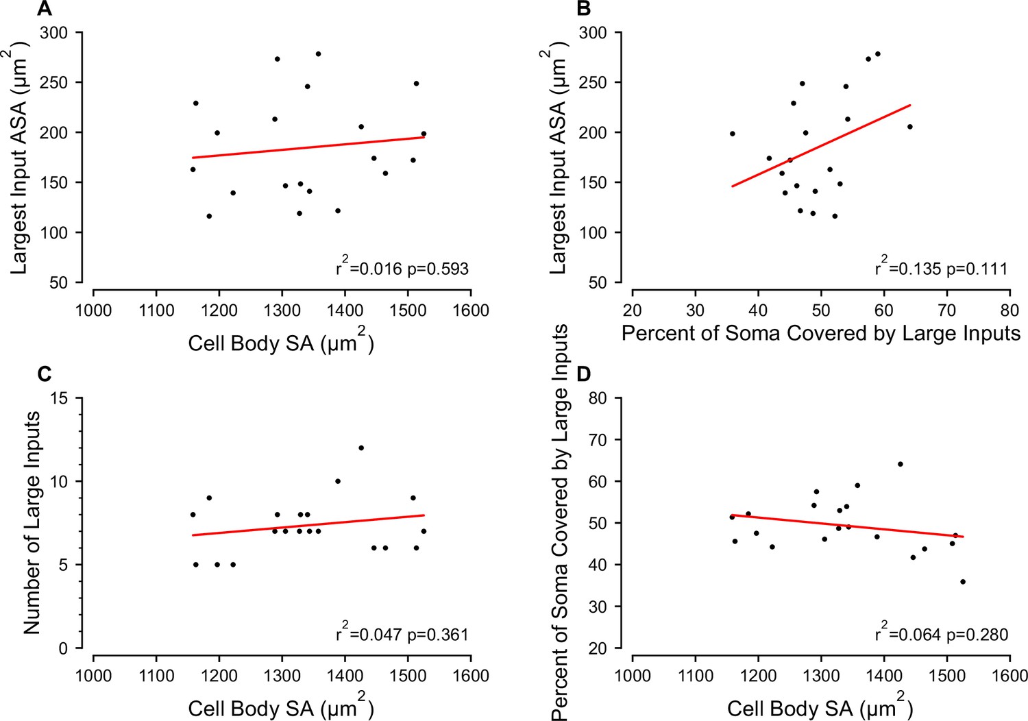
Morphological correlations for synapse and somatic area, related to Figure 2C and D.
Morphological correlations for synapse and somatic area, related to Figure 2C and D. (A) There was no relationship between cell body surface area (SA) and the apposed surface area (ASA) of the largest input. (B) There was a weak correlation between the somatic coverage by large inputs and the largest input area. (C) There was no correlation between cell body area and the number of large inputs. (D) There was no correlation between the area coverage by large inputs and the cell body area.
Figure 2—figure supplement 2
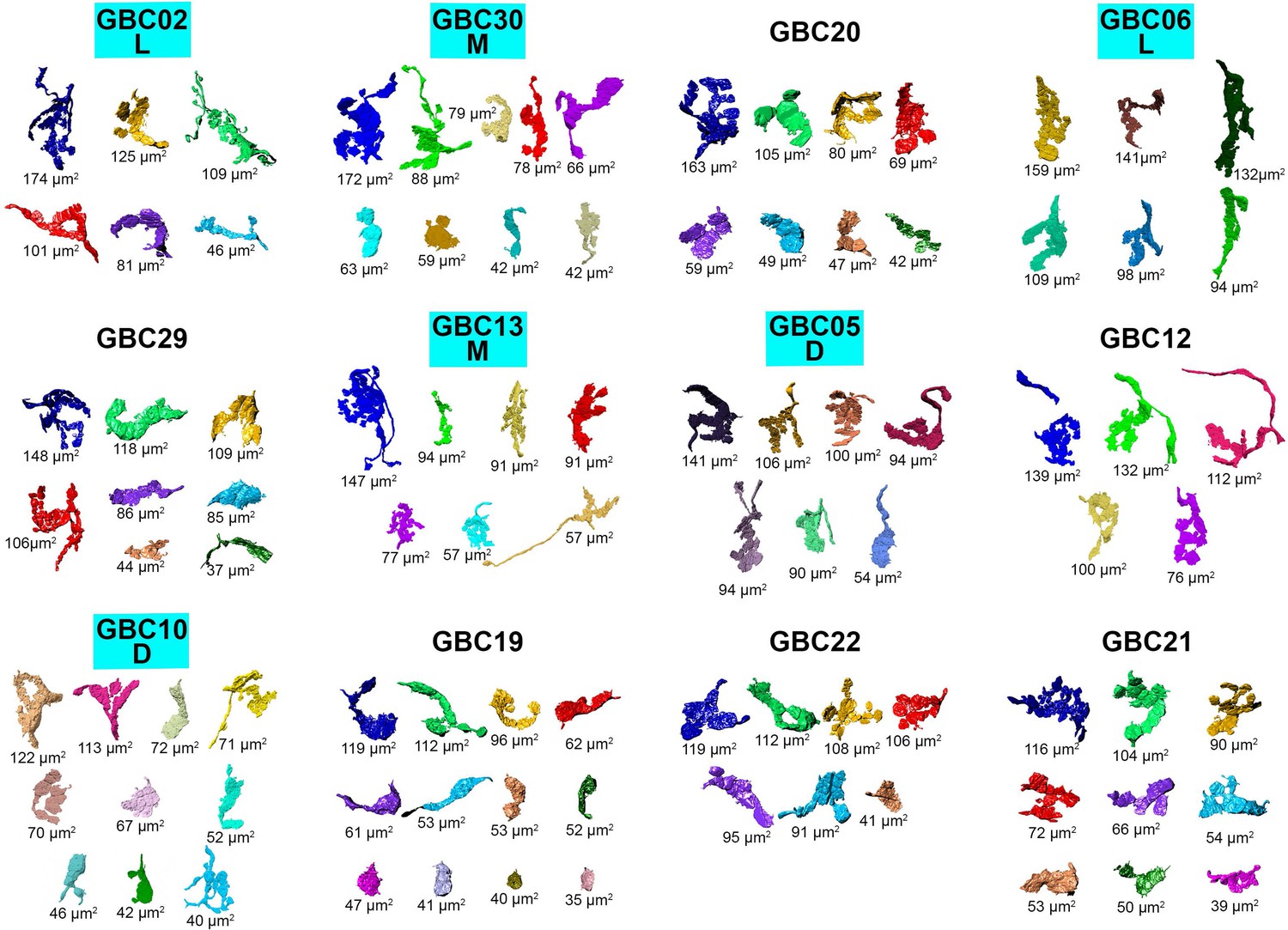
Large somatic terminals onto each globular bushy cell (GBC) that fit the Coincidence Detection model, related to Figure 2E.
Terminal groups are arranged from top left to bottom right in order of decreasing size of their largest input. Apposed surface area (ASA) is indicated next to each terminal. The number of terminals ranges from 5 (GBC12) to 12 (GBC19). Six of these GBCs (label enclosed in blue box) had dendrites fully reconstructed and were used for compartmental modeling. The extent of their local dendrite branching is indicated by L, low; M, moderate; D, dense. Scale bar omitted because these are 3D structures and most of the terminal would be out of the plane of the scale bar.
Figure 2—figure supplement 3
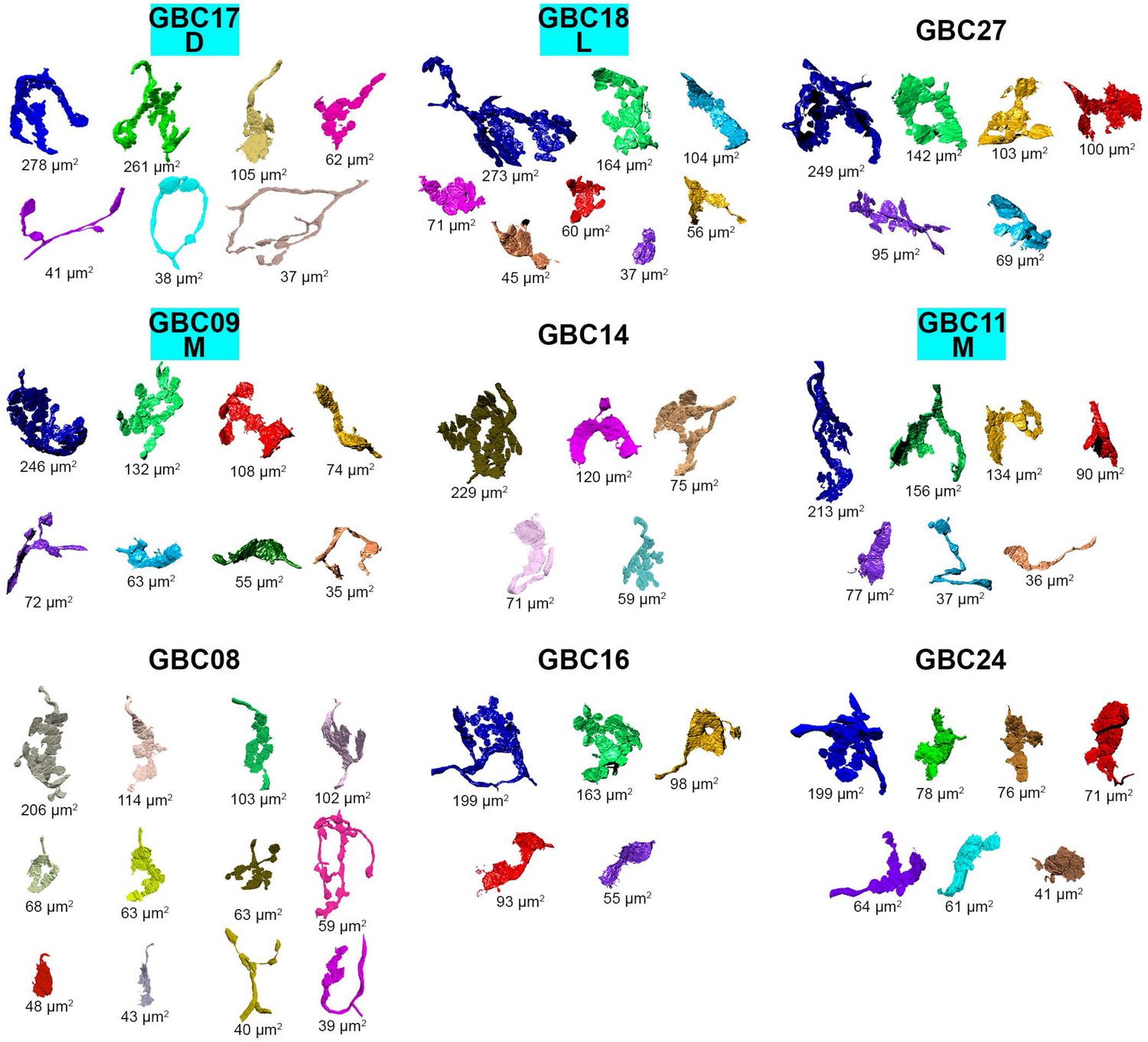
Large terminals onto each globular bushy cell (GBC) that fit the mixed Coincidence Detection/First-Arrival model, related to Figure 2F.
Terminal groups are arranged from top left to bottom right in order of decreasing size of their largest input. Apposed surface area (ASA) is indicated next to each terminal. The number of terminals ranges from 5 (GBC14, GBC16) to 12 (GBC08). Four of these GBCs (label enclosed in blue box) had dendrites fully reconstructed and were used for compartmental modeling. The extent of their local dendrite branching is indicated by L, low; M, moderate; D, dense. Scale bar omitted because these are 3D structures and most of the terminal would be out of the plane of the scale bar.
Figure 2—video 1
Exploration of all features of a globular bushy cell (GBC).
This video opens with a full view of GBC18, including its dendrites (red), cell body (beige), axon (pink), and all large somatic inputs (various colors). Note that the proximal dendrite and axon emerge from the same pole of the cell. Two endbulb terminals each extend onto the axon (blue arrows) and proximal dendrite (green arrows). The view pans around the cell body to reveal all somatic inputs and short segments of their axons.
Figure 3 with 1 supplement
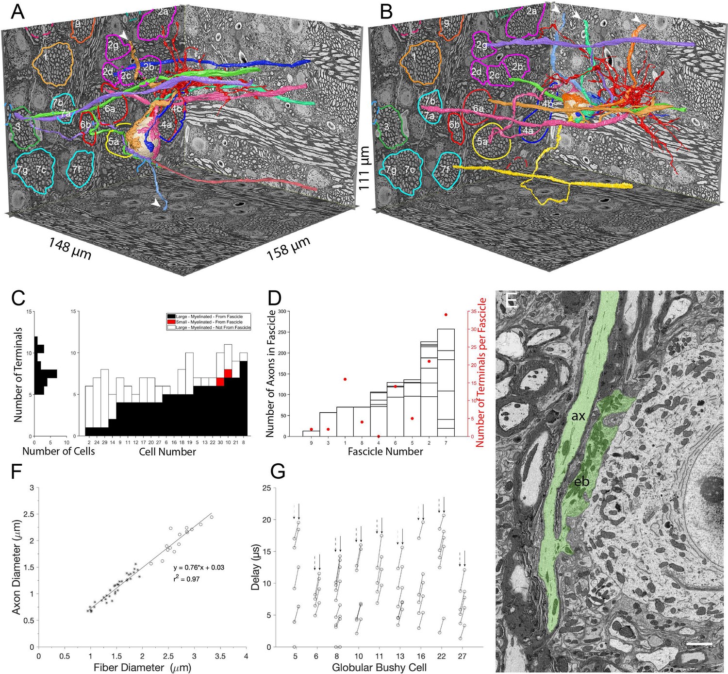
Large somatic terminals link to auditory nerve fibers (ANF) through myelinated branch axons of varying length and fascicle organization.
(A, B) ANFs and their branches leading to all large inputs for two representative cells. ANF, branch axon and large terminal have same color; each composite structure is a different color. Convergent inputs emerge from multiple fascicles (fascicles circled and named on back left EM wall), but at least two inputs emerge from the same fascicle for each cell (green, purple axons from fascicle 3 in panel (A); yellow, mauve axons from fascicle 7 and green, purple from fascicle 2 in panel (B)). Some branch axons leave image volume before parent ANF could be identified (white arrowheads). Globular bushy cell (GBC) bodies colored beige, dendrites red, axons mauve and exit volume at back, right EM wall; axon in panel A is evident in this field of view. (C) Stacked histogram of branch axons traced to parent ANF (black), branch axons exiting volume without connection to parent ANF (open), small terminals linked to parent ANF (red; included to illustrate these were a minority of endings), arranged by increasing number of large terminals traced to a parent ANF per GBC. GBCs with fewest branch connections to parent ANF (GBC02, 24, 29, 14) were at edge of image volume, so most branch axons could only be traced a short distance. Number of terminals per cell indicated in horizontal histogram at left. (D) Number of axons in each fascicle (left ordinate) and number of axons connected to endbulb terminals per fascicle (red symbols, right ordinate). (E) Example of en passant large terminal emerging directly from node of Ranvier in parent ANF. (F) Constant ratio of fiber diameter (axon +myelin) / axon diameter as demonstrated by linear fit to data. All branch fiber diameters (asterisks) were thinner than ANF parent axon diameters (open circles). (G) Selected cells for which most branch axons were traced to a parent ANF. Lines link the associated conduction delays from parent ANF branch location for each branch, computed using the individual fiber diameters (length / conduction velocity [leftmost circle, vertical dashed arrows] or values scaled by the axon length / axon diameter [rightmost circle, vertical solid arrow]). See Figure 3—video 1 for a detailed 3-D view of GBC11 and its inputs. Scalebar in (E) is 2 μm.
Figure 3—video 1
Exploration of all large somatic inputs onto a single globular bushy cell (GBC), their branch axons, and parent auditory nerve fibers.
This video opens with a full view of GBC11, including its dendrites (red), cell body (beige), axon (pink), all of its large somatic inputs (various colors), and the auditory nerve fibers (ANFs) from which those inputs originate. Somatic inputs and their axon branches, including the parent ANF, share the same color. The view zooms into the cell body, where a large terminal (red) extends onto the axon hillock and initial segment (blue arrow). The view pans around the cell body to show all large terminals, and an axon (cyan) that exited the volume before likely linking to an ANF is indicated by a red arrow. All except two terminals are then removed. The axons of these terminals are traced to branch points from their parent ANFs (magenta arrows). All inputs and their axons are replaced, and a second axon (green) that exits the volume before likely linking to an ANF is indicated (red arrow). The view pans to two ANFs (red and yellow) from the same nerve fascicle, and their branch points (magenta arrows). All other nerve terminals and axons are removed, and the two branch axons are traced to the cell body.
Figure 4 with 5 supplements
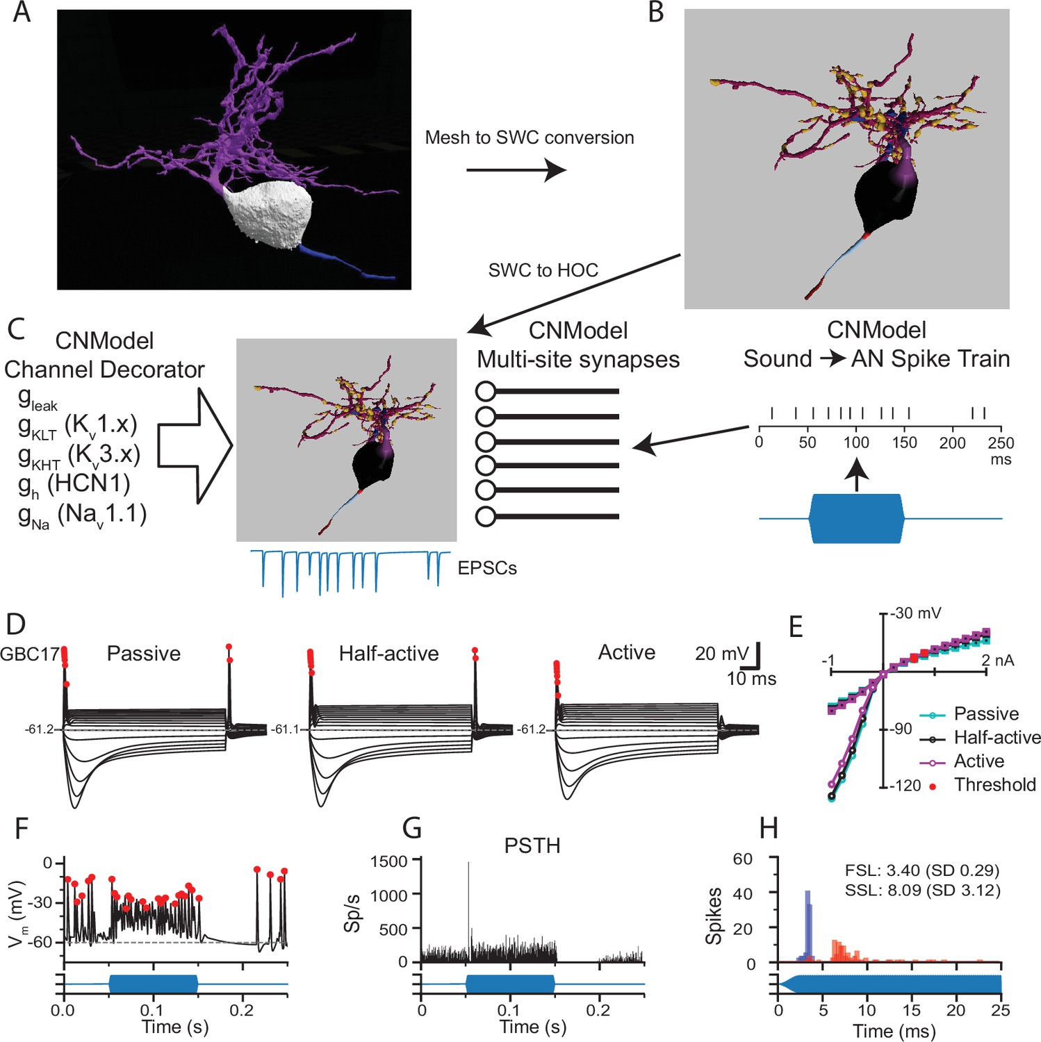
Pipeline to generate compartmental models for analysis of synaptic integration and electrical excitability from the mesh reconstructions of mouse VCN bushy neurons.
(A) The mesh representation of the volume EM segmentation was traced using syGlass virtual reality software to generate an SWC file consisting of locations, radii, and the identity of cell parts (B). In (B), the myelinated axon is dark red, the axon initial segment is light blue, the axon hillock is red, the soma is black, the primary dendrite is purple, dendritic hubs are blue, the secondary dendrite is dark magenta, and the swellings are gold. The mesh reconstruction and SWC reconstructions are shown from different viewpoints. See Figure 1—figure supplement 1 for all reconstructions. See Figure 4—video 1 for a 3D view of the mesh and reconstructions for GBC11. (C) The resulting SWC model is decorated with ion channels (see Figure 4—figure supplement 2 for approach), and receives inputs from multi-site synapses scaled by the apposed surface area of each ending. For simulations of auditory nerve input, sounds (blue) are converted to spike trains to drive synaptic release. (D). Comparison of responses to current pulses ranging from –1 to +2 nA for each dendrite decoration scheme. In the Passive scheme, the dendrites contain only leak channels; in the Active scheme, the dendrites are uniformly decorated with the same density of channels as in the soma. In the Half-active scheme, the dendritic channel density is one-half that of the soma. (E) Current voltage relationships for the 3 different decoration schemes shown in (D). Curves indicated with circles correspond to the peak voltage (exclusive of APs); curves indicated with squares correspond to the steady state voltage during the last 10ms of the current step. Red circles indicate the AP threshold. (F) Example of voltage response to a tone pip in this cell (Half-active model). Action potentials are marked with red dots, and are defined by rate of depolarization and amplitude (see Methods). (G) Peri-stimulus time histogram (PSTH) for 50 trials of responses to a 4 kHz 100 ms duration tone burst at 30 dB SPL. The model shows a primary-like with notch response. See Figure 4—figure supplement 4 for all tone burst responses. (H) First spike latency (FSL; blue) and second spike latency (SSL; red) histograms for the responses to the tone pips in G. (F,G,H) The stimulus timing is indicated in blue, below the traces and histograms.
Figure 4—figure supplement 1
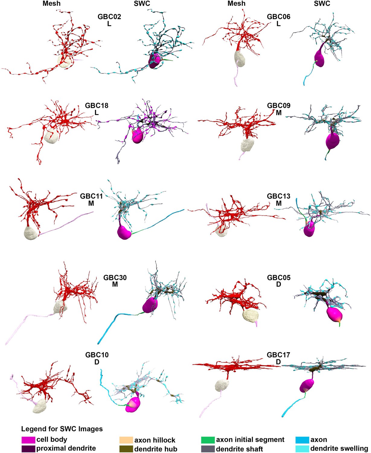
Segmented globular bushy cells (GBC) and their representations for compartmental modeling, related to Figure 4A and B.
Panels are labeled by cell number. For each GBC, the segmentation as computational meshes is depicted at left. Cell bodies are light grey, dendrites are red, and axons are pink. Cells are aligned to permit the most encompassing views of their dendrites. Meshes were converted to SWC format, which represents structures as a series of linked skeleton points with associated radius, using 3D virtual reality software (syGlass). The SWC representations are shown at right for each pair of images. Axon and dendrite subcompartments were annotated during SWC creation, which permitted quantification of their surface areas. Cells are clustered into three groups by the extent of local dendrite branching and braiding: low (L: GBCs 02, 06, 18), moderate (M: GBCs 09, 11, 13, 30), and dense (D: GBCs 05, 10, 17). Cellular compartments are color coded in the SWC files, as depicted in the legend. Scale bar is not included because it does not apply throughout the depth of the 3D structure. Images scaled to fit within figure panels so cells are pictured at different scales.
Figure 4—figure supplement 2
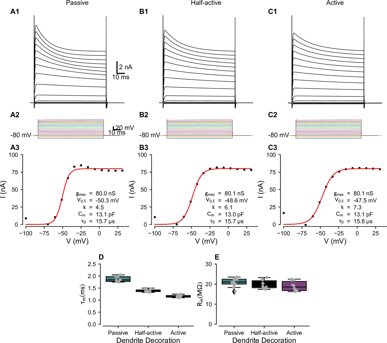
Conductance scaling using voltage clamp simulations for different patterns of dendrite decoration, related to Figure 4C.
Voltage-clamp simulations were used to compute total channel densities to match experimental data for different dendritic decoration configurations. (A) Passive dendrites. (A1): voltage clamp protocol with steps as in panel (A2). The transients at the start and end of the steps represent the charging of the cell membrane capacitance, which was not compensated in the model cell. (A3) Steady-state conductance calculated from the data in A1. The inset text indicates the fits to a Boltzmann function of the form:
where is the half-activation voltage and is the slope factor. is the cell capacitance, calculated from an exponential fit to the initial charging curve for small negative voltage steps, and is the clamp charging time constant (fastest time constant, representing somatic capacitance). (B) and (C) 1–3 are in the same format as (A1-3), with different channel decoration of the dendrites. (D) Input resistance measures from the 10 completely reconstructed cells for each of the decoration conditions from current-clamp simulations (see Figure 4—figure supplement 3). Boxplots: Shaded area indicates interquartile distances, whiskers indicate 5–95% confidence limits. (E) Time constant measurements from the 10 completely reconstructed cells for each of the decoration conditions from current clamp simulations. Boxplots are formatted as in (D). Scale bars in (A1) apply to (B1) and (C1). Scale bars in (A2) apply to (B2) and (C2).
Figure 4—figure supplement 3
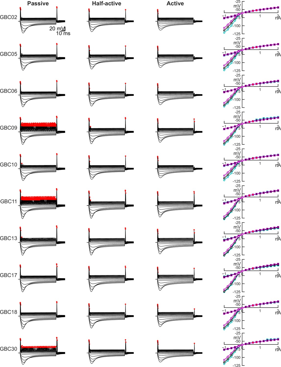
Current-clamp responses for all 10 complete bushy cells for each of the ion channel decoration conditions, related to Figure 4D and E.
All current-voltage relationships show traces from –1 to + 2 nA, in 0.2 nA steps. Action potentials are indicated by red dots. The calibration bar in the top row applies to all traces. The right-most column shows the steady-state current-voltage relationships (squares) and peak (circles, for hyperpolarization only) for each of the decoration conditions (Passive: cyan; Half-active: black, Active: magenta). Note that some model cells (GBCs 09, 11, 30) show small repetitive spikes with stronger depolarization with the passive dendrites. Most cells show spikes at anodal break, but these are attenuated or absent when the dendrites are fully active.
Figure 4—figure supplement 4
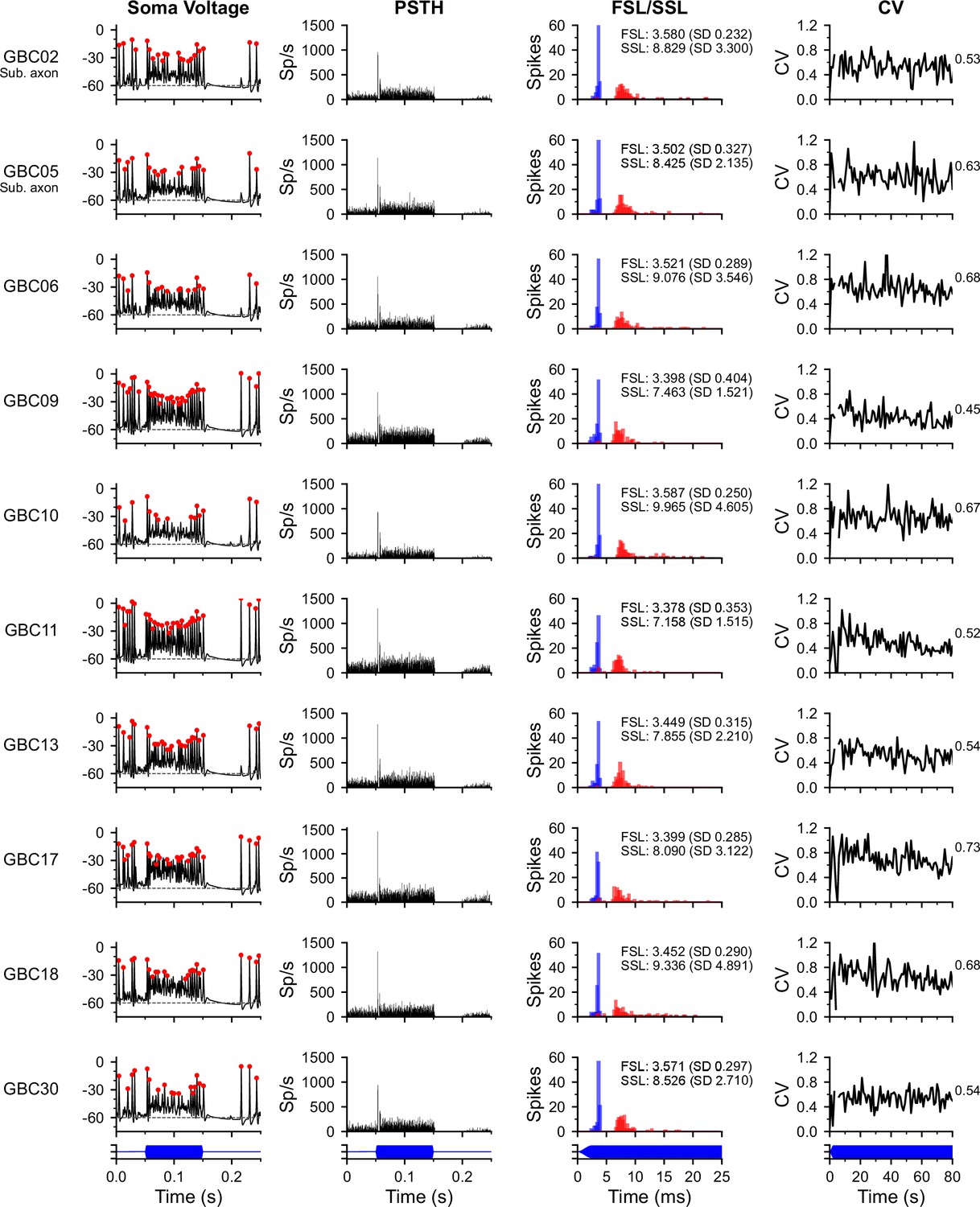
Peri-stimulus time histograms (PSTH), spike latencies and interpsike interval regularity in response to tone bursts at characteristic frequency, related to Figure 4F–H.
Each row shows the responses for one cell. The reconstructed axon of cells GBC02 and GBC05 left the volume prior to myelination and were simulated with a substitute axon (‘Sub. axon’) that had the average hillock, initial segment and myelinated axon lengths and diameters from the other eight cells. Otherwise, each cell was simulated using its own reconstructed axon. The first column (Soma Voltage) shows the somatic voltage for one trial for a stimulus at the characteristic frequency at 30 dB SPL. The stimulus starts after 50 ms and is 100 ms in duration. The PSTH column shows the spike rate as a function of time averaged over 100 repetitions of the tone pip, with 0.5 ms bins. The (FSL/SSL) column shows the first spike latency distribution (FSL, blue) and second spike latency distribution (SSL, red); text shows the mean and SD of the FSL and SSL. The rightmost column plots the coefficient of variation (CV) of interspike intervals corrected for a 0.7ms refractory period (CV). Intervals beginning less than 25 ms before the end of the stimulus were not included to minimize end effects. The CV value is indicated to the right of each plot. All CV values fall in the range of 0.3–0.7 reported for mouse primary-like neurons (Roos and May, 2012). The bottom row of plots shows the stimulus waveform timing for each column (blue).
Figure 4—video 1
Comparison of cell structures and regions between a 3D mesh and an SWC representation of a globular bushy cell (GBC).
This video opens with a full side-by side views of the GBC11 reconstruction (left), including its dendrites (red), cell body (beige), and axon (pink), and the SWC representation (right) of the same structures. The view then zooms into the cell body and axon, where the transition point from cell body to the axon (yellow arrow), the middle of the unmyelinated initial segment (green arrow), and the transition point where myelination of the axon begins (blue arrow) are indicated. Note that the diameter of the axon increases significantly where it is myelinated. Location of last paranodal loop of myelin is indicated by narrow, peach-colored band to right of the blue arrow on the SWC representation. The view then pans to a dorsolateral view of the cell, where a pink arrow indicates the proximal dendrite, and an orange arrow signifies the primary hub of the cell. The view then pans to a top-down location showing two secondary hubs (orange arrows). The view then shifts to reveal periodic dendrite swellings (three cyan arrows) separated by dendrite shafts (two red arrows). SWC color code: pink, cell body; axon hillock, orange; axon initial segment, light green; myelinated axon, light blue; proximal dendrite, maroon; dendrite hub, greenish-brown; dendrite swelling, cyan; dendrite shaft, gray.
Figure 5 with 2 supplements
Compartmental models predict sub- and suprathreshold inputs, efficacy dependence on dendrite surface area, and rate-dependent participation in spike generation.
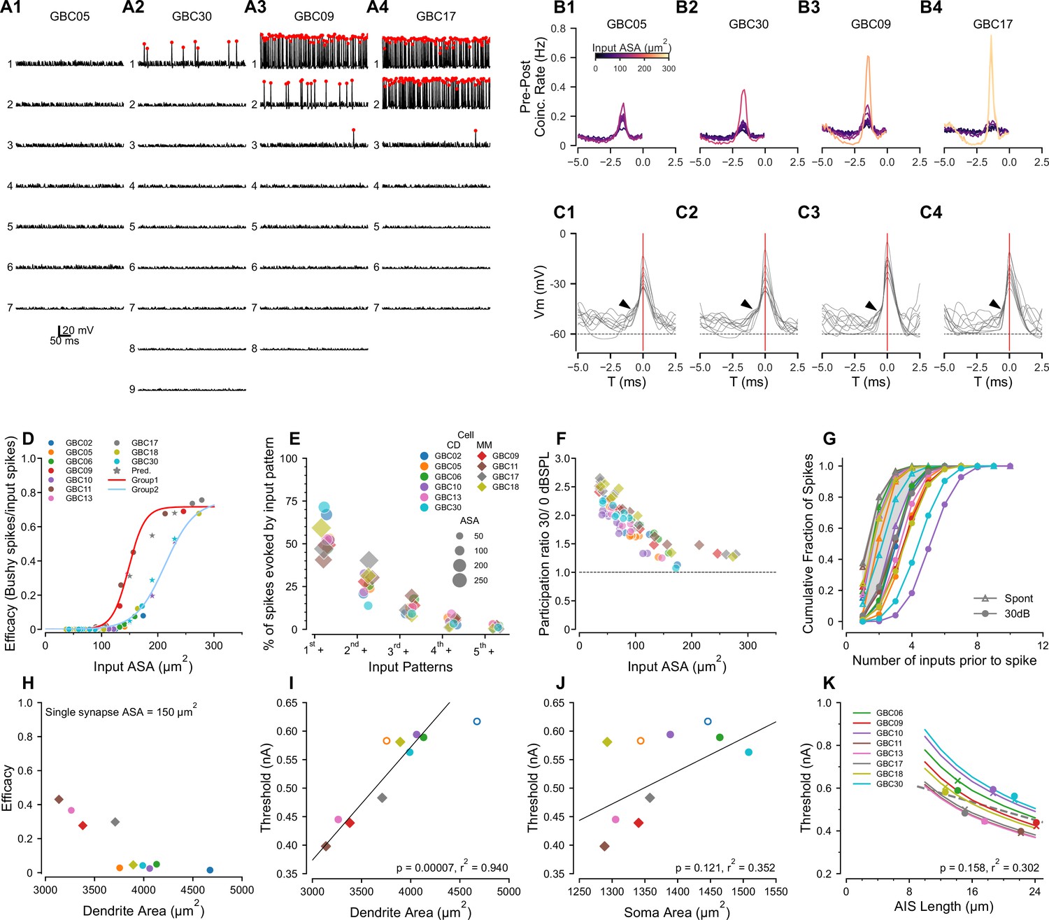
(A1-4) Simulations showing EPSPs and spikes in response to individual ANFs in 4 model globular busjy cells (GBCs) during a 30 dB SPL tone pip, arranged by efficacy of the largest input. Spikes indicated by red dots. Vertically, traces are ranked ordered by endbulb size. Responses for the other six cells are shown in Figure 5—figure supplement 1. (B1-4) Cross-correlations between postsynaptic spikes and spikes from each input ANF during responses to 30 dB SPL tones (all inputs active). Trace colors correspond to the ASA of each input (color bar in (B1)). See Figure 5—figure supplement 1 for cross-correlations for the other 6 cells. (C1-4): Voltage traces aligned on the spike peaks for each of the 4 cells in (B). Postsynaptic spikes without another spike within the preceding 5ms were selected to show the subthreshold voltage trajectory more clearly. Zero time (0ms; indicated by vertical red line) is aligned at the action potential (AP) peak and corresponds to the 0 time in (B1-4). Arrowheads indicate EPSPs preceding the SP in panels (C1-3); arrowhead in C4 shows APs emerging directly from the baseline, indicating suprathreshold inputs. (D) GBCs could be divided into two groups based on the pattern of efficacy growth with input size. GBCs 09, 11, 13 and 17 formed one group, and GBCs 02, 05, 06, 10, 18, and 30 formed a second group with overall lower efficacy. The red line is a best fit logistic function to the higher efficacy group. The blue line is the logistic fit to the lower efficacy group. Stars indicate test ASA-efficacy points, supporting membership in the lower efficacy group for cells 10 and 30. (E) Comparison of the patterns of individual inputs that generate spikes. Ordinate: indicates spikes driven by the largest input plus any other inputs. indicates spikes driven by the second largest input plus any smaller inputs, excluding spikes in which the largest input was active. indicates spikes driven by the third largest input plus any smaller inputs, but not the first and second largest inputs. indicates contributions from the fourth largest input plus any smaller inputs, but not the 3 largest. indicates contributions from the fifth largest input plus any smaller inputs, but not the 4 largest. Colors and symbols are coded to individual cells, here grouped according to predicted coincidence mode or mixed-mode input patterns as shown in Figure 2—figure supplement 2 and Figure 2—figure supplement 3. See Figure 5—figure supplement 2 for a additional summaries of spikes driven by different input patterns. (F) The participation of weaker inputs (smaller terminal area) is increased during driven activity at 30 dB SPL relative to participation during spontaneous activity. The dashed line indicates equal participation at the two levels. Each input is plotted separately. Colors and symbols are coded to individual cells as in (D). (G) Cumulative distribution of the number of inputs driving postsynaptic spikes during spontaneous activity and at 30 dB SPL. The color for each cell is the same as in the legend in (D). Symbols correspond to the stimulus condition. (H) Efficacy for a single 150 μm2 input is inversely related to dendrite surface area. (I) Dendrite area and action potential threshold are highly correlated. Open circles (GBC02 and GBC05) indicate thresholds calculated using the average AIS length, but are not included in the regression. Colors and symbols as in (D). (J) Soma area and action potential threshold are not well correlated. Open symbols are as in (I). (K) Variation of AIS length using the averaged axon morphology reveals an inverse relationship to spike threshold for all cells (lines). Crosses indicate thresholds interpolated onto the lines for the averaged axon simulations; circles indicate thresholds measured in each cell with their own axon. Cells GBC02 and GBC05 are omitted because AIS length is not known. Across the cell population, the thresholds are only weakly correlated with AIS length (linear regression indicated by dashed grey line). Colors as in (E).
Figure 5—figure supplement 1
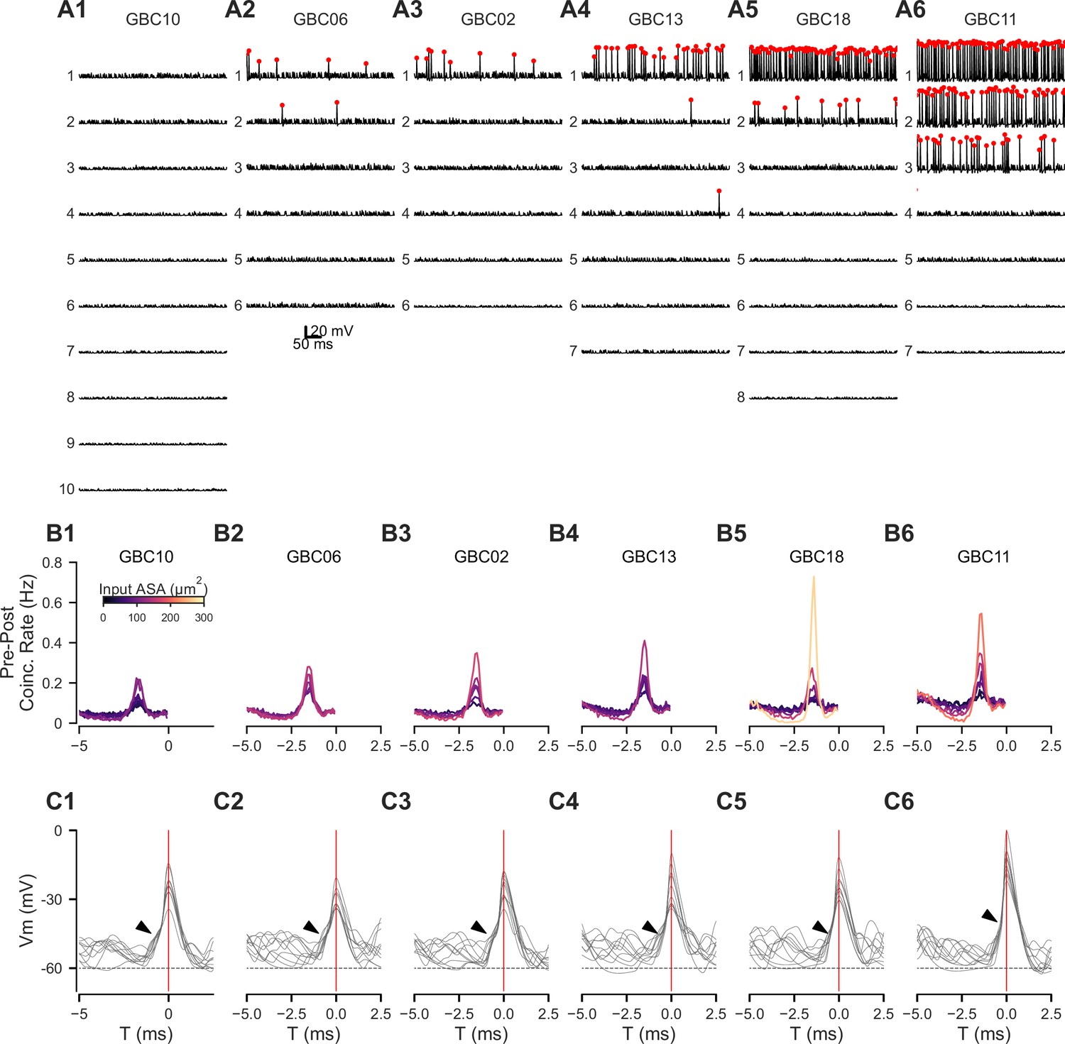
Cross-correlation plots for six additional modeled cells, related to Figure 5A–C.
Cross-correlation plots for six additional modeled cells , related to Figure 5A–C. Each cell is plotted in the same format as in Figure 5A, D and E. Summary information is presented in panels Figure 5D–J.
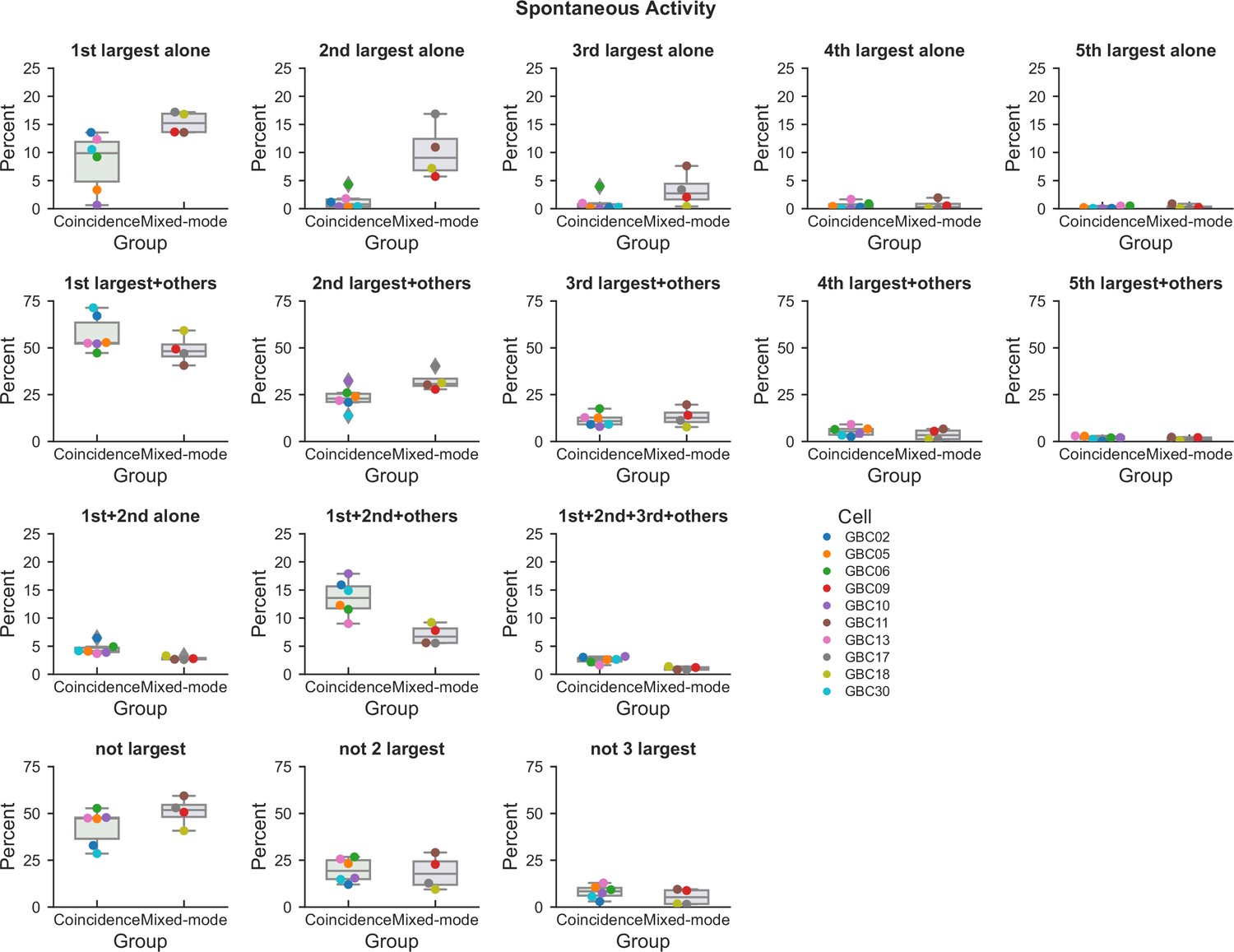
Figure 5—figure supplement 2
Contributions of different input patterns to postsynaptic spiking, related to Figure 5E.
For each panel, the contributions of different combinations of inputs measured in globular bushy cells GBC02, GBC05, GBC06, GBC10, GBC13, GBC30 (‘Coincidence’ group) an in the mixed-mode group of cells GBC09, GBC11, GBC17, GBC18 (‘Mixed-mode’ group). The panels are titled according to the particular patterns of input, and plot the percent of postsynaptic spikes that were generated by each pattern. Cell colors are the same as in other figures. The bars show the median, interquartile distances, and 5–95% whiskers. Points that fall outside of the expected distribution are indicated with diamonds. Results were calculated during spontaneous activity. Individual cells are noted by the color in the legend.
Figure 6 with 4 supplements
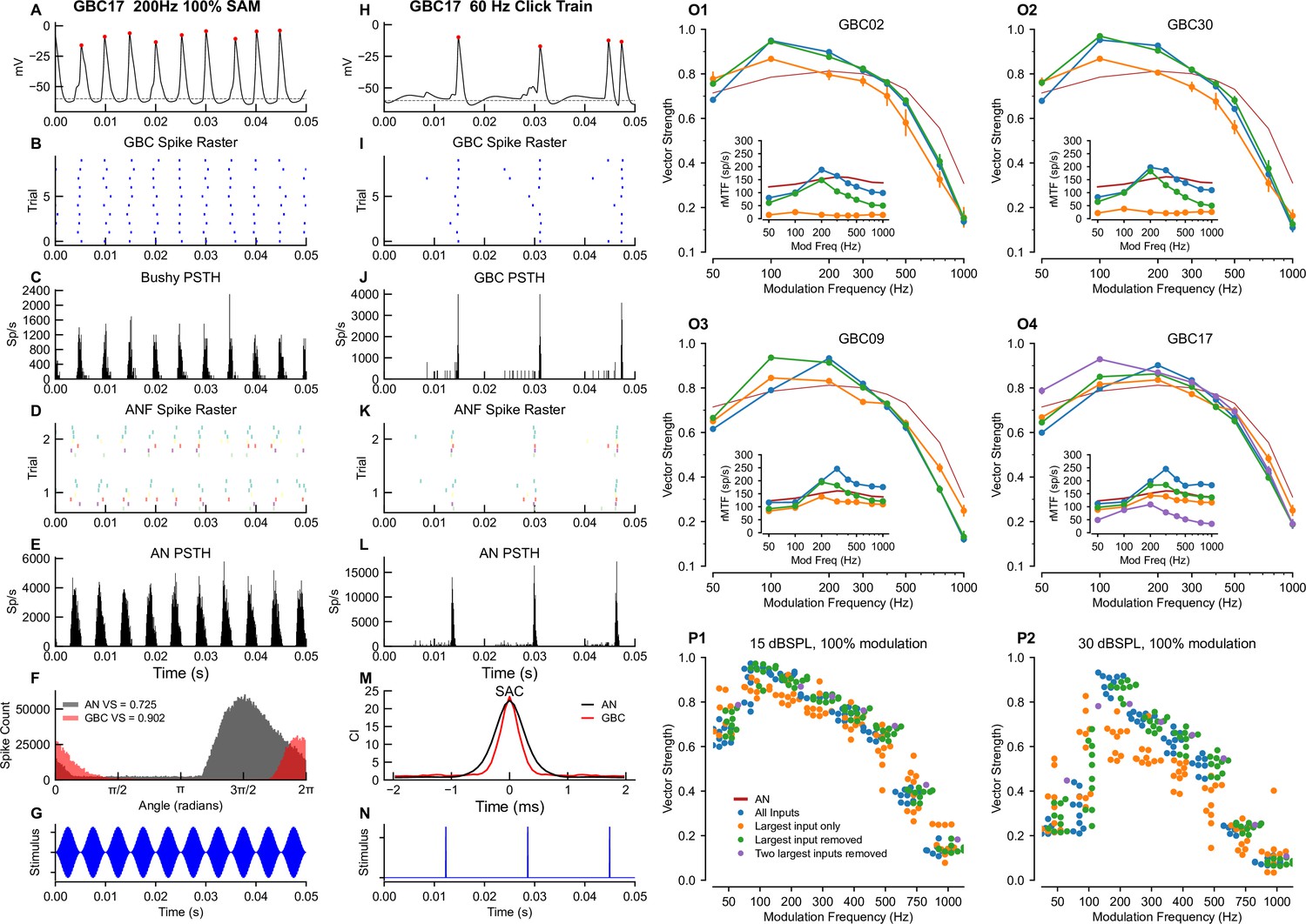
Temporal and rate modulation transfer functions and entrainment to clicks can exceed ANF values and differ between coincidence detection and mixed mode cells.
Left column (A–G): Example of entrainment to 100% modulated SAM at 200 Hz, at 15 dB SPL. The sound level was chosen to be near the maximum for phase locking to the envelope in ANFs (see Figure 6—figure supplement 1). (A) Voltage showing spiking during a 150ms window starting 300ms into a 1 second long stimulus. (B) Spike raster for 100 trials shows precise firing. (C) PSTH for the spike raster in (B). (D) Spike raster for all ANF inputs across a subset of 2 trials. Inputs are color coded by ASA. (E) PSTH for the ANF. (F) Superimposition of the phase histograms for the GBC (black) and all of its ANF inputs (red). (G) Stimulus waveform. Center column (H–N): responses to a 50 Hz click train at 30 dB SPL. (H) GBC membrane potential. (I) Raster plot of spikes across 25 trials. (J) PSTH showing spike times from I. (K) ANF spike raster shows the ANFs responding to the clicks. (L) PSTH of ANF firing. (M) The shuffled autocorrelation index shows that temporal precision is greater (smaller half-width) in the GBC than in the ANs. See Figure 6—figure supplement 4 for SAC analysis of other cells. (N) Click stimulus waveform. Right column (O–P): Summary plots of vector strength. (O1-4) Vector strength as a function of modulation frequency at 15 dB SPL for 3 (4 for GBC17) different input configurations. Vertical lines indicate the SD of the VS computed as described in the Methods. Insets show the rate modulation transfer function (rMTF) for each of the input configurations. Red line: average ANF VS and rMTF (insets). See Figure 6—figure supplement 2 for the other cells. Figure 6—figure supplement 3 shows spike entrainment, another measure of temporal processing. The legend in (P1) applies to all panels in (O) and (P). (P) Scatter plot across all cells showing VS as a function of modulation frequency for 3 (4 for GBC17) different input configurations. (P1) VS at 15 dB SPL. (P2) VS at 30 dB SPL.
Figure 6—figure supplement 1
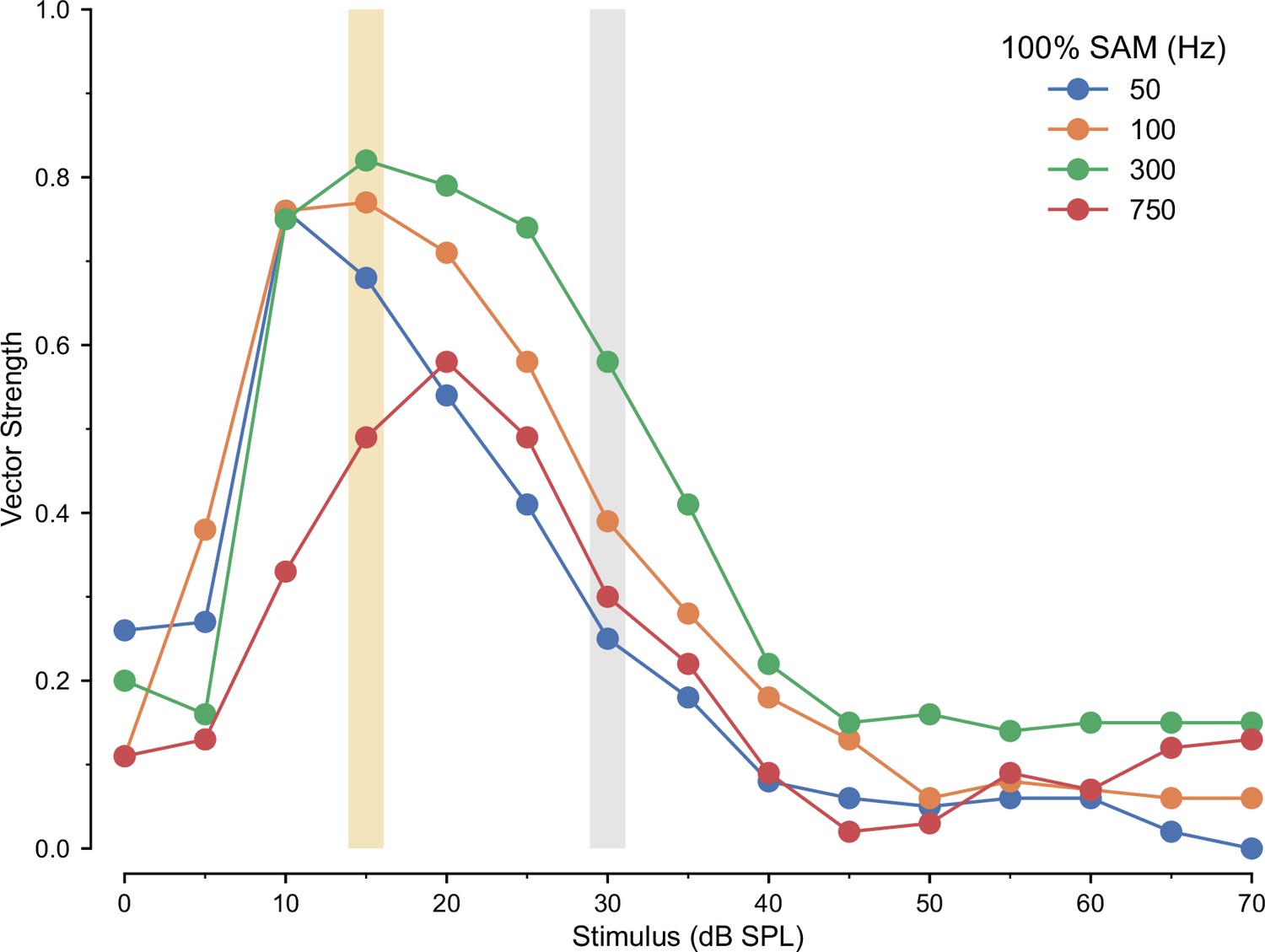
Spike synchronization to stimulus envelope as a function of average stimulus intensity in ANF inputs, related to Figure 6F and P1 and P2.
Vector strength of response to 100% SAM across frequency for the ANF model. Carrier frequency was 16 kHz. Color bars indicate 15 dB SPL (gold) used in Figure 6, O1-4 and P1, and 30 dB SPL (gray), as used in Figure 6, P2.
Figure 6—figure supplement 2
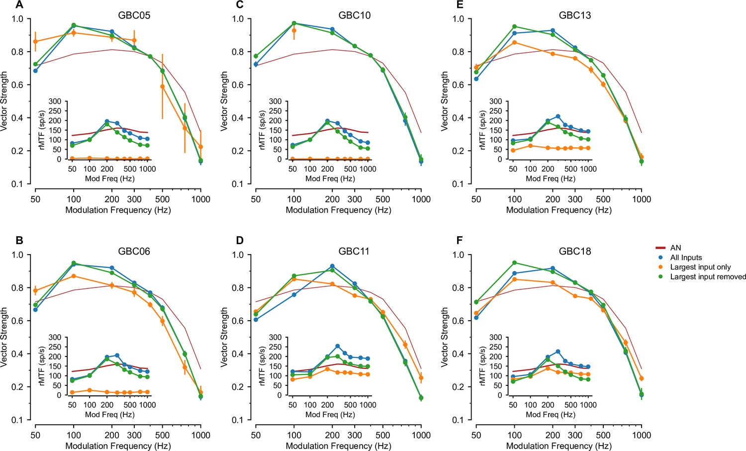
Vector strength of the 6 other globular bushy cells (GBCs) in response to 100% SAM tones at frequencies from 50 to 1000 Hz on a 16kHz carrier at 15 dB SPL, related to Figure 6O1-4.
These simulation results are also included in Figure 6P1. Each plot shows vector strength for 3 (or in the case of GBC 17, 4) different synaptic input configurations. The vertical lines indicate the SD of the vector strength (VS) computed as described in the Materials and methods. Insets show the rate modulation transfer function (rMTF; see Materials and methods for calculation) across SAM frequencies for each synaptic configuration. (A) Cell GBC05, (B) Cell GBC06, (C) Cell GBC10, (D) Cell GBC11, (E) Cell GBC13, (F) Cell GBC18. GBC10 had too few spikes with only the largest input to compute VS except at 100 Hz.
Figure 6—figure supplement 3
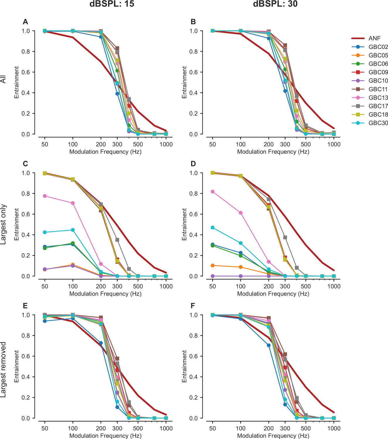
Spike entrainment across all globular bushy cells (GBCs) at 15 and 30 dB SPL when different combinations of inputs are active, related to Figure 6P1-2.
Spike entrainment across all globular bushy cells (GBCs) at 15 and 30 dB SPL when different combinations of inputs are active, related to Figure 6P1-2. Entrainment could exceed ANF values when all (A, B) or all except the largest (E, F) inputs were active. The largest inputs alone (C, D) showed entrainment less than or equal to that of ANFs. Symbols: Mixed-mode cells:, coincidence-detection cells: ○. ANFs: dark red line.
Figure 6—figure supplement 4
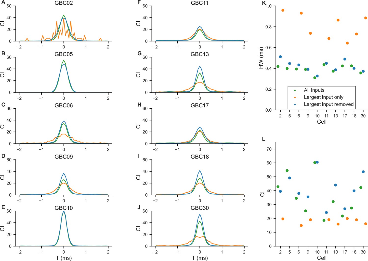
Shuffled autocorrelations (SACs) in response to click trains show importance of weaker inputs in improving temporal precision, related to Figure 6M.
SACs were computed for click evoked spike trains as shown in Figure 6. (A–J) SACs computed for each of the globular bushy cells (GBCs) for 3 different input configurations (colors are indicated in panel K). For GBC05 (B) and GBC10 (E), there were insufficient spikes in the largest input only condition for the SAC calculation. (K) Half-width of the SAC for each cell and configuration, computed from Gaussian fits to the SACs in panels (A–J). (L) SAC correlation index (CI) at 0 time for each cell and configuration.
Figure 7 with 1 supplement
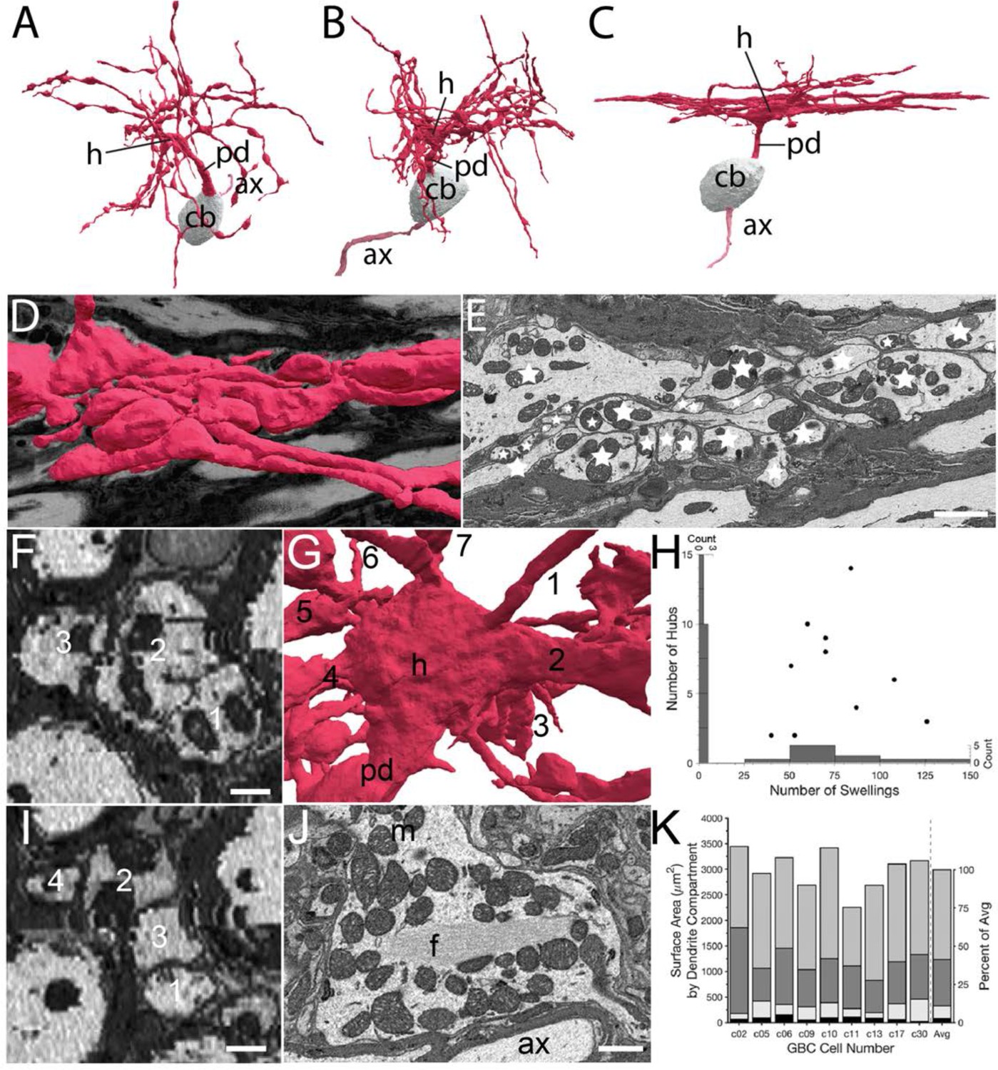
Volume EM reveals unique dendrite hub structures and branching patterns.
(A–C). Dendrites vary in density of local branching and braiding of branches from the same cell, exhibiting (A) little, (B) medium or (C) dense branching and braiding. (D–E). Tangential view of dense braiding, showing (D) reconstruction of multiple branches in contact with one another and (E) a single EM cross-section illustrating contact among the multitude of branches (individual branches identified with stars). (F, I). Two locations of cross-cut braided dendrites showing intertwining as change in location of branches (numbers) along the length of the braid. Images are lower resolution because viewing perspective is rotated 90 from image plane. (G). Reconstruction of dendrite hub (h) and its multiple branches (7 are visible and numbered in this image). (H). Swellings and hubs are prominent features of GBC dendrites. Histograms of numbers of swellings and hubs plotted along abscissa and ordinate, respectively. (J). Core of many hubs is defined by a network of filaments (f); also see Figure 7—figure supplement 1. Many mitochondria are found in hubs and can be in apparent contact with the filament network. (K). Partitioning of dendrite surface area reveals that proximal dendrite (black), hub (light grey), swelling (dark grey) and shaft (medium grey) compartments, in increasing order, contribute to the total surface area for each cell. Averaged values indicated in stacked histogram, to right of vertical dashed line, as percent of total surface area ((right ordinate), and aligned with mean sizes on left ordinate). Scale bars: E, 2 microns; F, I, 0.5 microns; J, 1 micron.
Figure 7—figure supplement 1
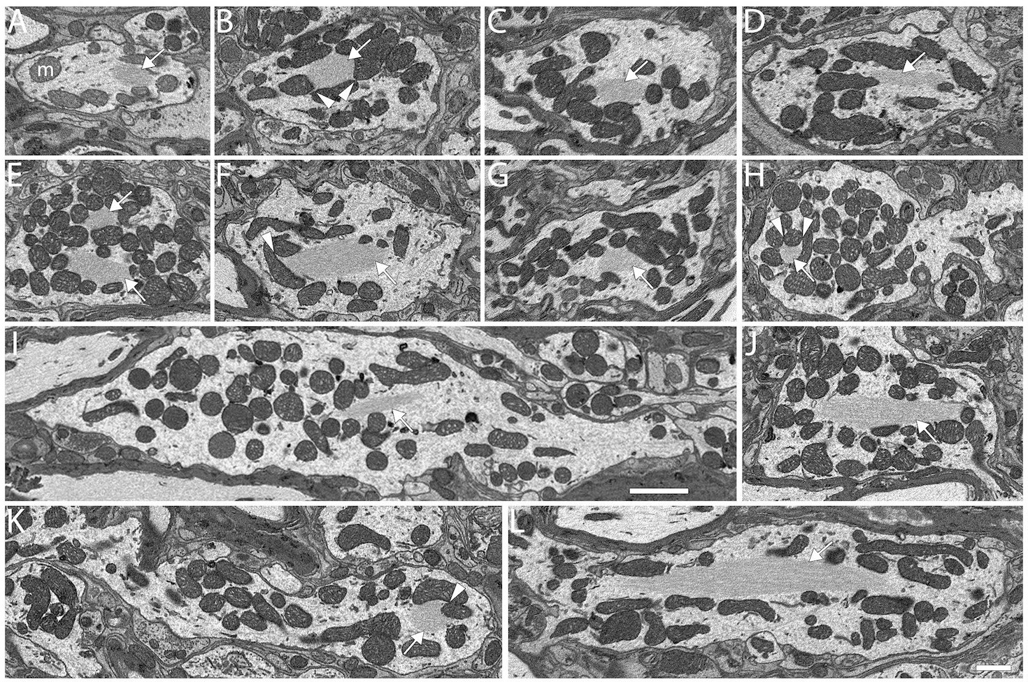
Dendritic Hubs, related to Figure 7G and J.
Filament core (white arrows) in primary globular bushy cell (GBC) hubs and dendrite of one multipolar cell (MC) A-L. MC04, GBCs 05, 14, 27, 08, 10, 09, 24, 17, 30, 29, 16. Filaments appear in close apposition to mitochondrion outer membranes and can fill narrow spaces defined by those membranes (white arrowheads). Scale bar = 1 micron in panel L applies to all panels except panel I scale bar = 2 µm.
Figure 8 with 1 supplement
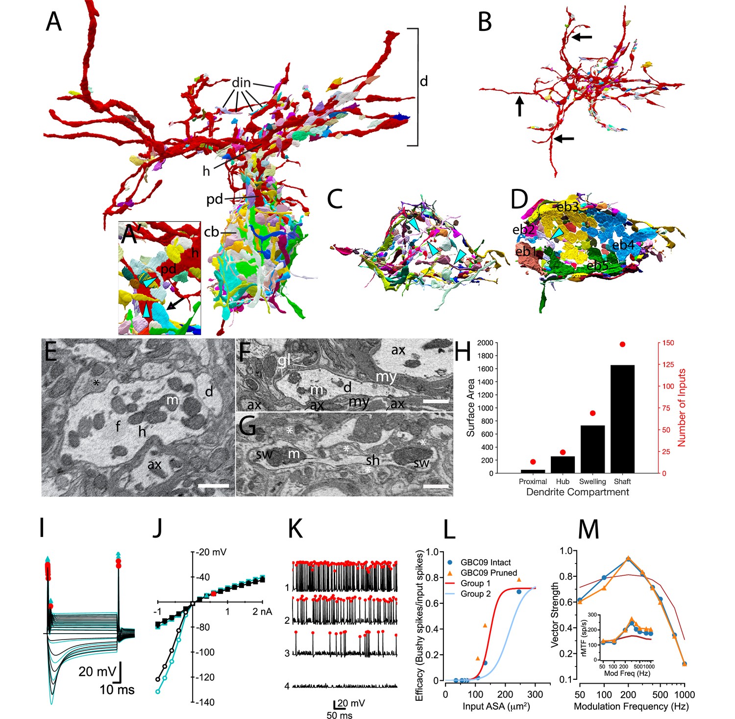
Synaptic map of GBC with modeled effects of removing non-innervated dendrites.
(A) GBC09 oriented to show inputs (din) to dendrites (red, d), including proximal dendrite (pd), primary hub (h) and cell body (gray, cb). Nerve terminals are colored randomly. Terminals contacting dendrites at higher order sites than the primary hub are bouton-type of varying volume. (A) Closeup view of pd reveals high density innervation by primarily bouton terminals that can be linked by small connections (cyan arrowheads), and extension of a somatic endbulb onto the basal dendrite (arrow). (B) Top-down view of dendrites only, illustrating that some branches are not innervated (longest non-innervated branches indicated by arrows) and that other branches are innervated at varying density. (C) Bouton terminals innervate all regions of the cb surface. Some boutons are linked by narrow connectors (cyan arrowheads). The cb is removed to better reveal circumferential innervation. (D) Inside-out view of cb innervation by endbulbs (ebs; each is numbered and a different color) reveals that they cover most of the cb surface. Cb removed to reveal synaptic face of ebs. (E) Cross section through primary hub (h), showing filamentous core (f), mitochondria (m), input terminals (asterisks), and contact with dendrite of another cell. (F) Non-innervated dendrites (d) can be embedded in bundles of myelinated (my) axons (ax), and also ensheathed by glial cells (gl) and their processes (lines). (G) Both dendrite swellings (sw) and shafts (sh) can be innervated (asterisks). (H) Proximal dendrites are innervated at highest density (number of inputs / surface area), and hubs, swellings and shafts are innervated at similar density. Scale bars: 1 μm in each panel. (I–M) Simulation results after pruning the non-innervated dendrites from this cell. (I) Voltage responses to current pulses, as in Figure 4—figure supplement 3, comparing the intact cell (black traces) with one in which non-innervated have been pruned (cyan traces). (J) IV relationship of data in (I) Cyan triangle indicates the spike threshold with the dendrites pruned compared to the intact cell (red circle). (K) Spikes elicited by the 4 largest individual inputs at 30 dB SPL with the dendrites pruned (compare to data shown in Figure 4A3). (L) Comparison of the efficacy of individual inputs between intact and pruned cell as a function of ASA. The red and light blue lines (Group1 and Group2) are reproduced from Figure 4D. (M) Comparison of VS to SAM tones in the intact and pruned configuration. Inset: Rate modulation transfer function (rMTF) comparing intact and pruned dendritic trees. Colors and symbols match legend in (L). Dark red line is the rMTF for the auditory nerve input.
Figure 8—video 1
Exploration of a globular bushy cell (GBC) and all of its synaptic inputs.
This video opens with a full view of GBC09, including its dendrites (red), cell body (beige), axon (pink), all somatic inputs (various colors), and all dendritic inputs (various colors). The cell undergoes a full rotation to display all of the inputs. The view zooms into the axon region, and rotates to illustrate all inputs onto the axon, including extensions of two large terminals (blue arrows pointing to purple and yellow terminals). The view zooms out to show the entire cell, the dendrites are removed, and the cell body is tilted. A cut plane passes from the edge to the middle of the cell, providing an inside-out view of the nearly complete synaptic coverage of the cell body. Large terminals are indicated by cyan arrows. All cellular elements are added, and the view shifts to reveal dense innervation of the proximal dendrite, including an extension of a large terminal (green terminal indicated by green arrow). The perspective shifts to a top-down view of the dendrites, indicating several dendritic branches (yellow arrows) that lack synaptic inputs.
Tables
Key resources table
| Reagent type (species) or resource | Designation | Source or reference | Identifiers | Additional information |
|---|---|---|---|---|
| Strain, strain background (Mouse, male) | FVB/NJ | Jackson Laboratory | RRID:IMSR_JAX:001800 | JAX Stock # 001800 |
| Chemical compound, drug | 2,2,2 Tribromoethanol | TCI Chemicals | T1420 | |
| Chemical compound, drug | tert-Amyl Alcohol | TCI Chemicals | P0059 | |
| Chemical compound, drug | xylocaine | Sigma | PHR1257 | |
| Chemical compound, drug | heparin | Sigma | H5515 | |
| Chemical compound, drug | Cacodylic acid | EM Sciences | RT12201 | |
| Chemical compound, drug | glutarldeyhde | EM Sciences | 100503–972 | |
| Chemical compound, drug | Paraformaldehyde - EM grade | source | RT19208 | |
| Chemical compound, drug | calcium chloride | Sigma | 223506 | |
| Chemical compound, drug | potassium ferrocyanide | EM Sciences | RT20150 | |
| Chemical compound, drug | Nanopure water | Barnstead International | D11901 | |
| Chemical compound, drug | osmium tetroxide | EM Sciences | 19132 | |
| Chemical compound, drug | thiocarbohydrazide | EM Sciences | 21900 | |
| Chemical compound, drug | uranyl acetate | EM Sciences | 22400 | |
| Chemical compound, drug | lead nitrate | EM Sciences | 17900 | |
| Chemical compound, drug | ethanol | Fisher Chemical | A962P-4 | |
| Chemical compound, drug | acetone | Fisher Chemical | A18-4 | |
| Chemical compound, drug | Gold/palladium sputter target | Ted Pella | 91651 | |
| Chemical compound, drug | Durcopan resin | EM Sciences | 14040 | |
| Chemical compound, drug | Aclar strips | EM Sciences | 50425–10 | |
| Chemical compound, drug | Silver paint | Ted Pella | 16031 | |
| Software, algorithm | Seg3D | The NIH/NIGMS Center for Integrative Biomedical Computing | RRID:SCR_002552 | https://www.seg3d.org |
| Software, algorithm | Blender 2.9 | The Blender Foundation | RRID:SCR_008606 | https://www.blender.org |
| Software, algorithm | syGlass 1.7 | IstoVisio, Inc | RRID:SCR_017961 | https://www.syglass.io |
| Software, algorithm | nrrd_tools | https://digitalcommons.usf.edu/etd/9543 | None | https://github.com/MCKersting12/nrrd_tools |
| Software, algorithm | NEURON V7.7-V8.0 | DOI:10.1017/CBO9780511541612 | RRID:SCR_005393 | http://www.neuron.yale.edu |
| Software, algorithm | Python V3.7–3.10 | Python Software Foundation | RRID:SCR_008394 | https://www.python.org |
| Software, algorithm | cnmodel | PMID:29331233 | None | https://github.com/cnmodel |
| Software, algorithm | Prism V9.3 | GraphPad, Inc | RRID:SCR_002798 | https://www.graphpad.com |
| Software, algorithm | MATLAB R2022a | MathWorks, Inc | RRID:SCR_001622 | https://www.mathworks.com |
| Software, algorithm | Adobe Illustrator V26.0.3 | Adobe, Inc | RRID:SCR_010279 | https://www.adobe.com/ products/illustrator.html |
| Other | Merlin Scanning Electron Microscope | Zeiss Group, Oberkochen, Germany | None | https://www.zeiss.com |
| Other | National Center for Microscopy and Imaging Research | University of California at San Diego | RRID:SCR_016627 | https://ncmir.ucsd.edu |
Table 1
Densities of channels used to decorate the axon compartments of bushy cells.
Values are given as ratios relative to the standard decoration of the somatic conductances.
| Decoration Type | |||
|---|---|---|---|
| Channel | Myelinated axon | AIS | AH |
| 0.0 | 100.0 | 5.0 | |
| 0.01 | 2.0 | 1.0 | |
| 0.01 | 1.0 | 1.0 | |
| 0.0 | 0.5 | 0.0 | |
| 0.00025 | 1.0 | 1.0 | |
Table 2
Densities of channels in dendrites for three models.
Values are relative to somatic conductance. Leak is in mS/cm2.
| Dendrite Decoration Type | |||
|---|---|---|---|
| Channel | Passive | Half-Active | Active |
| 0.0 | 0.5 | 1.0 | |
| 0.0 | 0.5 | 1.0 | |
| 0.0 | 0.5 | 1.0 | |
| 0.0 | 0.5 | 1.0 | |
| 0.0693 | 0.0693 | 0.1385 | |
Additional files
Download links
A two-part list of links to download the article, or parts of the article, in various formats.
Downloads (link to download the article as PDF)
Open citations (links to open the citations from this article in various online reference manager services)
Cite this article (links to download the citations from this article in formats compatible with various reference manager tools)
High-resolution volumetric imaging constrains compartmental models to explore synaptic integration and temporal processing by cochlear nucleus globular bushy cells
eLife 12:e83393.
https://doi.org/10.7554/eLife.83393


