Competitive interactions between culturable bacteria are highly non-additive
- Institute of Environmental Sciences, Hebrew University, Israel
Figures
Figure 1 with 5 supplements
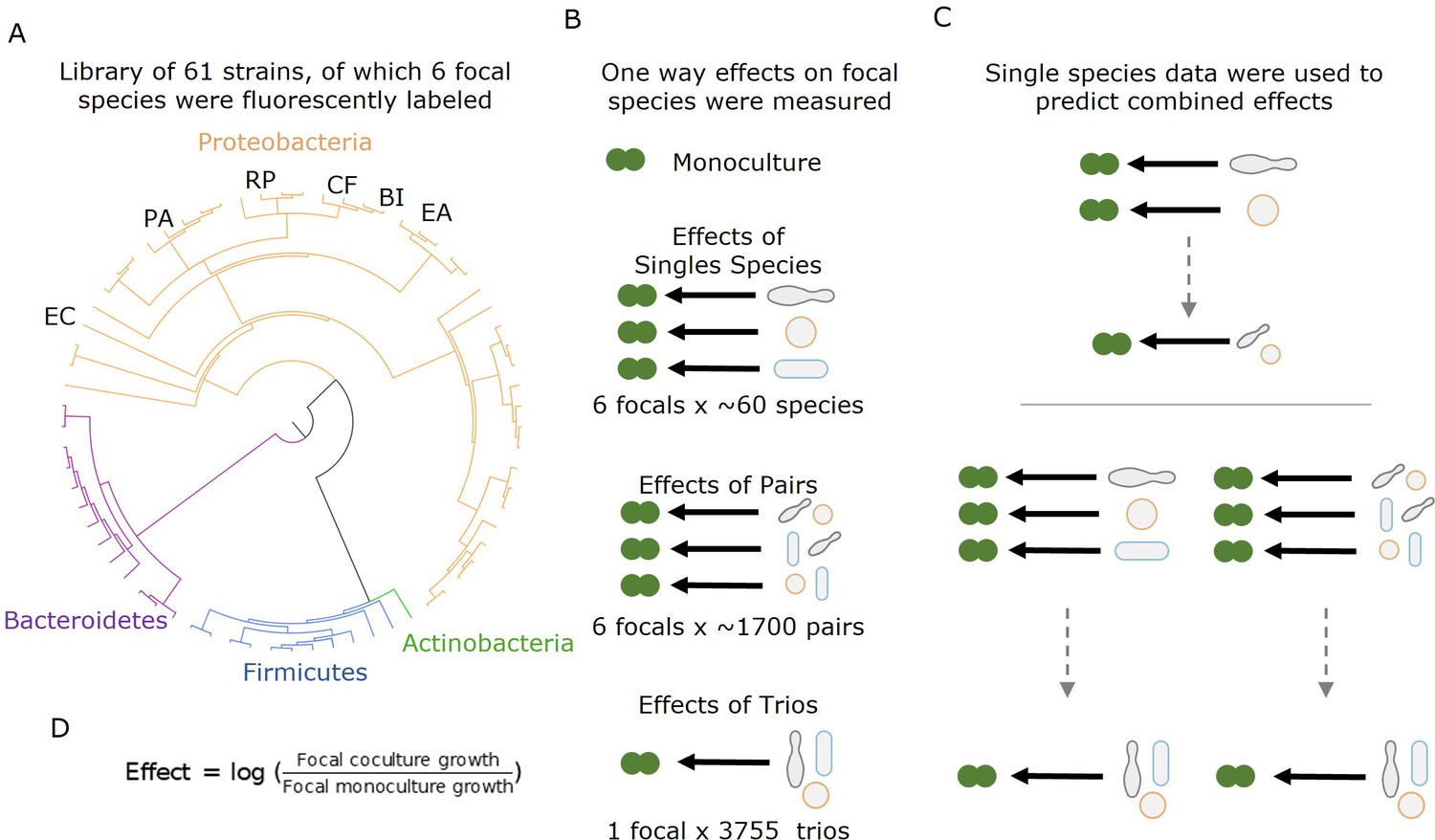
Measuring effects of 61 affecting species, and their pairs and trios on 6 focal species.
(A) A library of 61 soil and leaf-associated bacterial strains was used in this experiment. All strains are from four orders: Proteobacteria (orange), Firmicutes (blue), Bacteroidetes (purple), and Actinobacteria (green) (full list in Supplementary file 1a, Source data 1). Also, 6 of the 61 species were labeled with GFP and used as ‘focal’ species whose growth was tested in the presence of the other isolates (affecting species). These strains are labeled on the phylogenetic tree (Escherichia coli [EC], Ewingella americana [EA], Raoultella planticola [RP], Buttiauxella izardii [BI], Citrobacter freundii [CF], and Pantoea agglomerans [PA].) (B) Each focal species was grown in monoculture, with (between 18 and 52) single affecting species, and (between 153 and 1464) pairs of affecting species. Additionally, E. coli was grown with 3009 trios of affecting species. (C) Effects of pairs and trios were then predicted using the effects of single species and single species and pairs, respectively. Predictions were made using three different models: additive, mean, and strongest (detailed in ‘Results’ and ‘Materials and methods’). (D) Equation used for calculating the effect of an affecting species on the focal species.
Figure 1—figure supplement 1
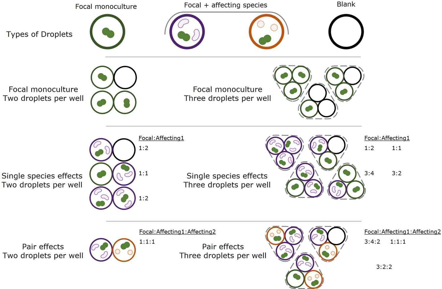
Species in each droplet and well in kChip experiments.
Droplets contained one of three different types of samples: (1) focal monoculture, containing only the focal species, (2) coculture of focal species and a single affecting species at an optical densities ratio of 2:1, and (3) blank samples, with media but no bacterial cells. Based on which two or three droplets (depending on the experimental setup) each well contained either a focal monoculture, one, two or three, affecting species. Similar communities started at different initial densities based on how many monoculture or blank droplets were in the well, but as shown in Figure 1—figure supplement 2, initial densities did not influence the effect on the focal. Ratios of focal species to affecting species 1 and 2 are detailed for different well setups.
Figure 1—figure supplement 2
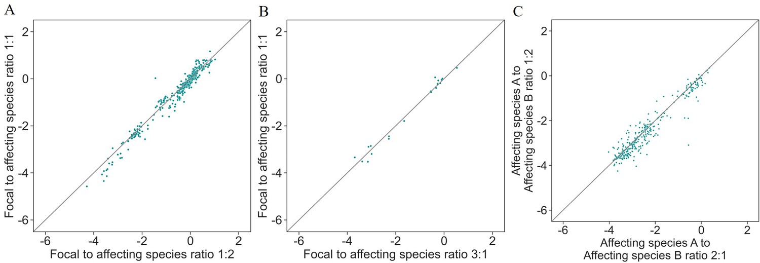
Effects on focal species are independent of initial species' density.
Correlation between different ratios of initial optical density in each well. (A) Different ratios of focal to affecting species based on whether there were two droplets containing the affecting species or one and one focal monoculture droplet: nRMSE = 0.22. (B) Different ratios of focal to affecting species based on whether there were three droplets containing the affecting species or one and two focal monoculture droplets: nRMSE = 0.16. (C) Different ratios of affecting species based on whether there were two droplets containing affecting species A and one droplet containing affecting species B or vice versa: nRMSE = 0.24.
Figure 1—figure supplement 3
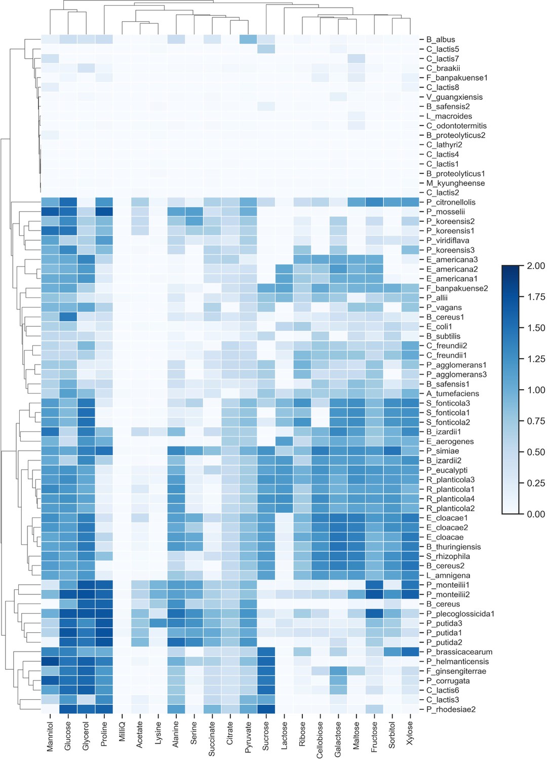
Carbon source utilization profiles for bacterial strains.
Each strain’s yield on 20 different carbon sources, assayed after 48 hr. Growth values are calculated as mean OD600 measurement from three replicates and were background-subtracted (media with no bacteria).
Figure 1—figure supplement 4
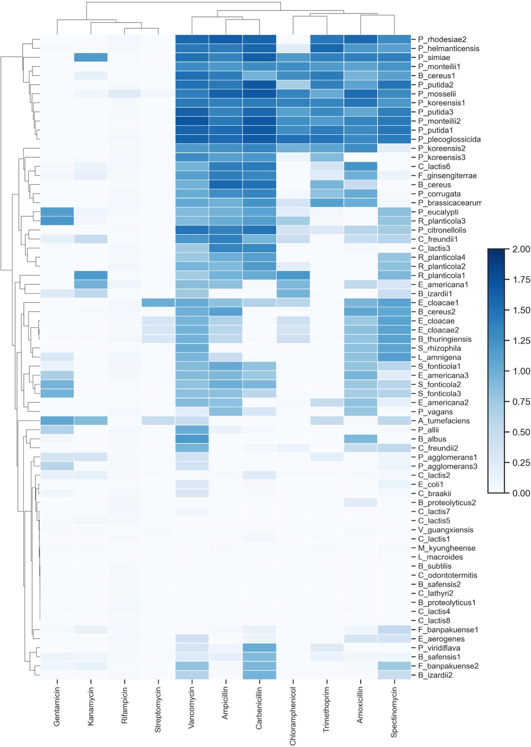
Antibiotic resistance profiles for bacterial strains.
Each strain’s ability to grow on 11 different antibiotics after 48 hr. Growth values are calculated as mean OD600 measurement from three replicates and were background-subtracted (media with no bacteria).
Figure 1—figure supplement 5
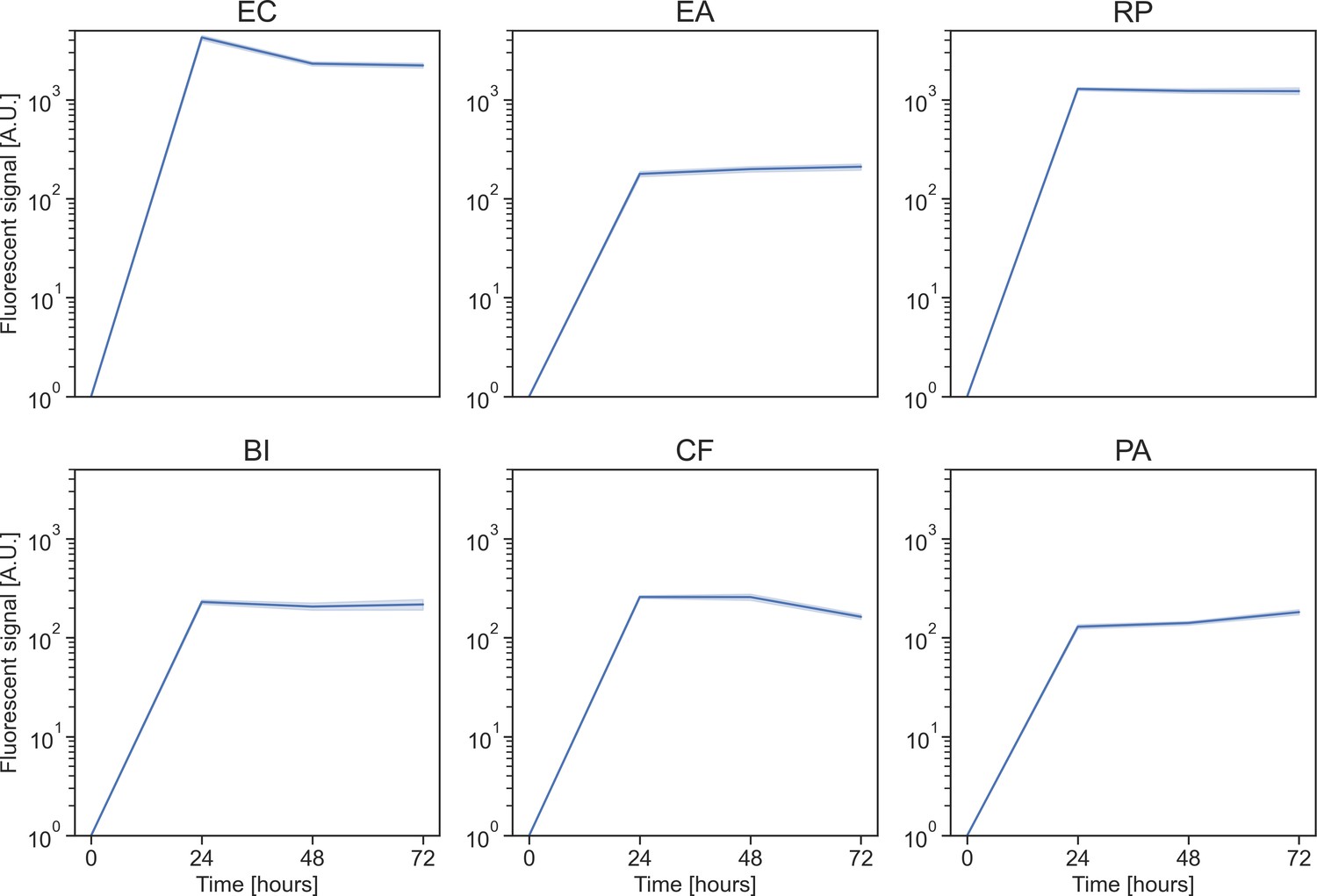
Growth dynamics of focal species in monoculture.
Growth in kChip of each focal strain in monoculture over 72 hr. Growth is measured by fluorescent signal and each well is normalized to the value at the beginning of the experiment (all signals at time zero are equal to one). The solid line represents the mean, and the shaded area the 95% confidence interval.
Figure 2 with 1 supplement
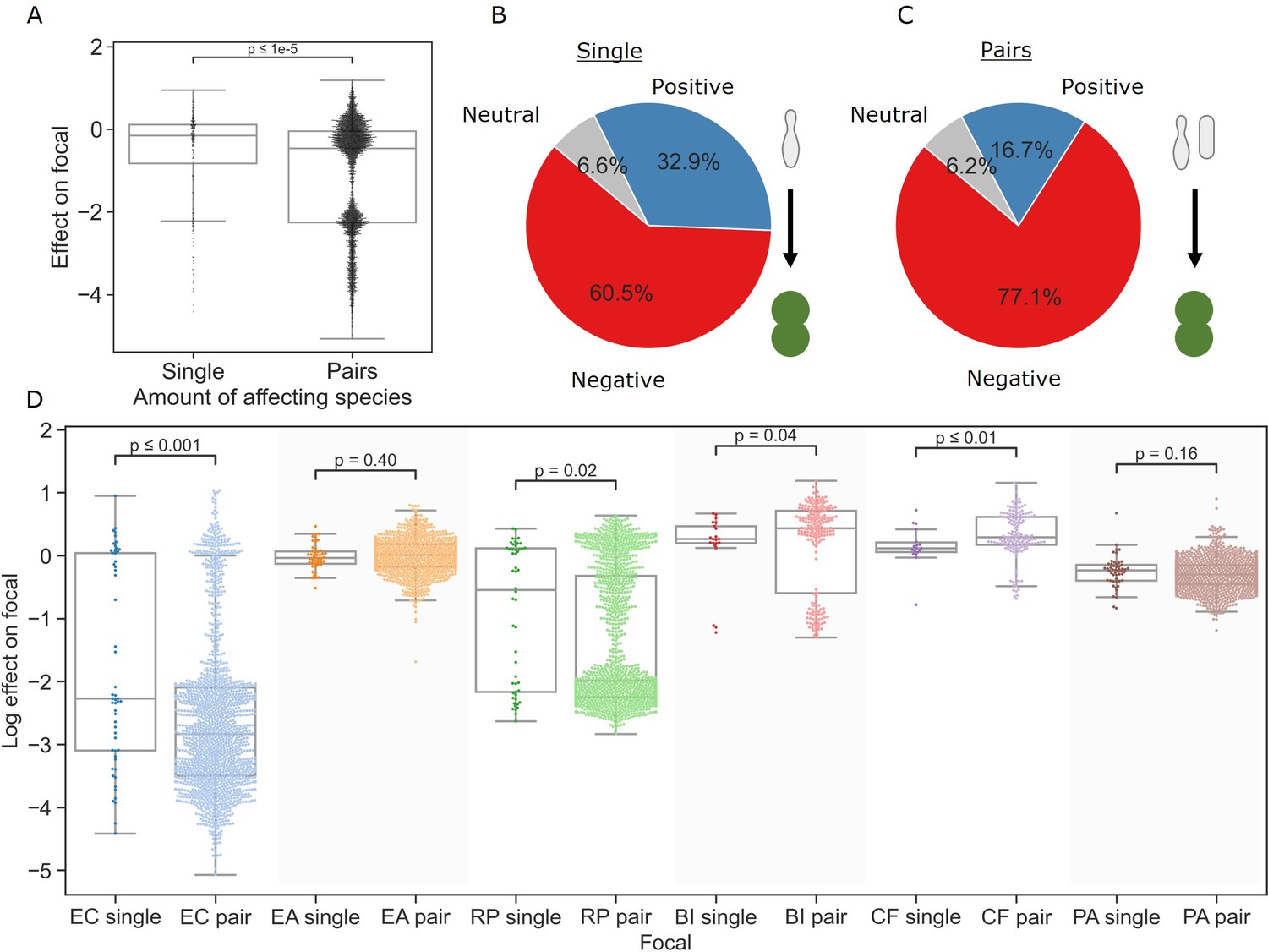
Pairs of affecting species have stronger effects than single species.
(A) Distribution of the effects of single and pairs of affecting species on all focal species. Mann–Whitney–Wilcoxon test two-sided, p-value = 1e-9. Dots show individual effects, solid lines represent the median, boxes represent the interquartile range, and whiskers are expanded to include values no further than 1.5× interquartile range. (B, C) Distribution of qualitative effects of single and pairs of affecting species respectively on all focal species. (D) Distribution of the effect of single and pairs of affecting species for each focal species individually. Dots represent individual measurements, solid lines represent the median, boxes represent the interquartile range, and whiskers are expanded to include values no further than 1.5× interquartile range. Mann–Whitney–Wilcoxon test two-sided tests were performed for each focal species, and p-values are shown on the graph.
Figure 2—figure supplement 1
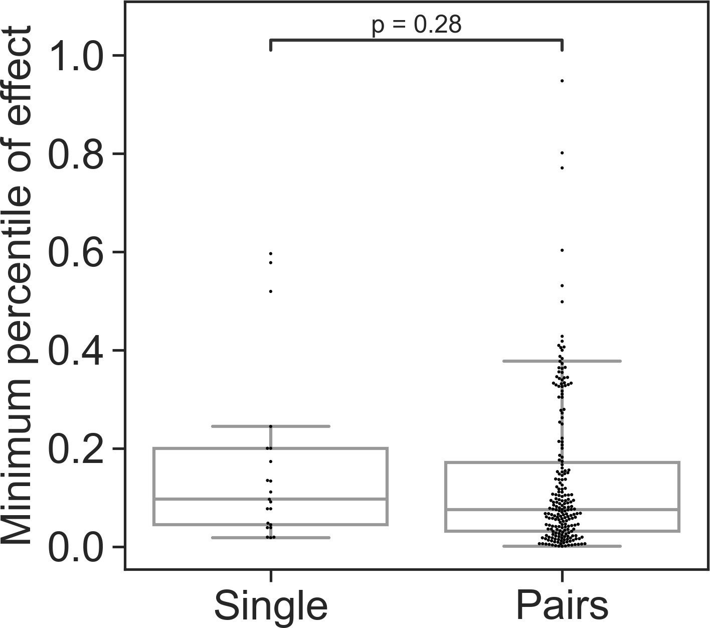
Minimal effect of single strains and pairs across multiple focals.
Distributions of the weakest effect of each individual species and pairs measured as the percentile within the distributions of effects for a single focal species (for affecting species that were measured against atleast four focal species). For each species or pair, the minimal value from all focals was taken to generate the above distributions. Sign was not regarded in this calculation, only strength of the effect. Dots represent individual measurements, solid lines represent the median, boxes represent the interquartile range, and whiskers are expanded to include values no further than 1.5× interquartile range. Mann–Whitney–Wilcoxon test two-sided tests were performed, and p-value is shown on the graph.
Figure 3 with 6 supplements
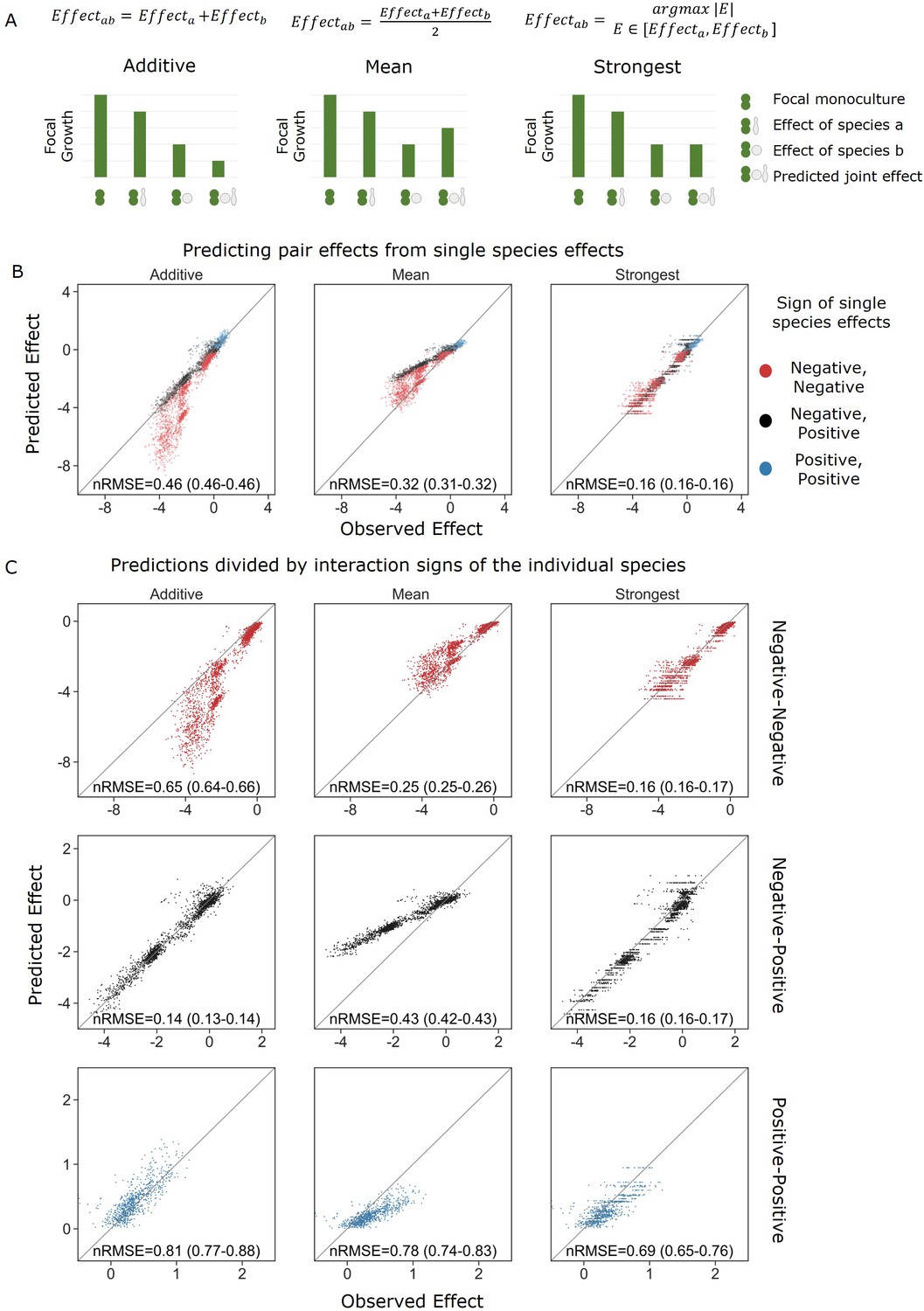
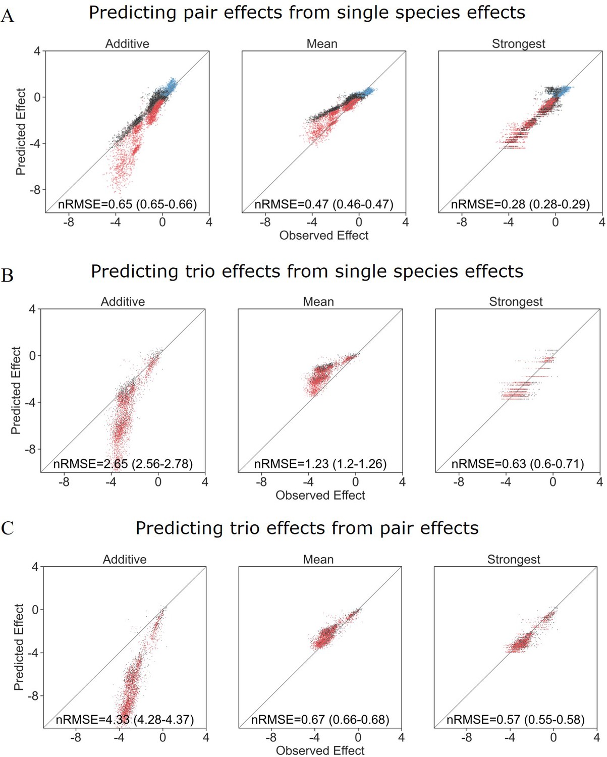
Strongest single-species effect offers the most accurate model for the combined effect of two species.
(A) Graphical representation for each model. The additive model assumes that the effects of each species will accumulate, indicating they are acting independently, and are unaffected by one another. The mean model assumes the combined effect will be an average of the two single-species effects. The final model, strongest effect, assumes that whichever species had a stronger effect on its own will determine the joint effect when paired with an additional species. The y-axis represents the growth of the focal species in different conditions, and in these examples effects are negative. (B) Comparison of predicted effects and the experimental data, with their respective root mean squared error normalized to the interquartile range of the observed data (nRMSE). nRMSE values are calculated from 1000 bootstrapped datasets and represent the median and interquartile range in parentheses (see ‘Materials and methods’). Each dot represents the joint effect of a pair of affecting species on a focal species. Colors indicate the signs of the measured effects of the individual affecting species. (C) Similar to panel (B), but data is stratified by interaction signs of the individual affecting species.
Figure 3—figure supplement 1
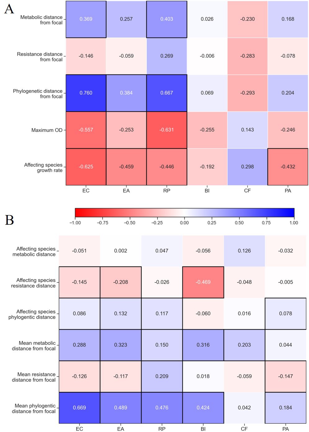
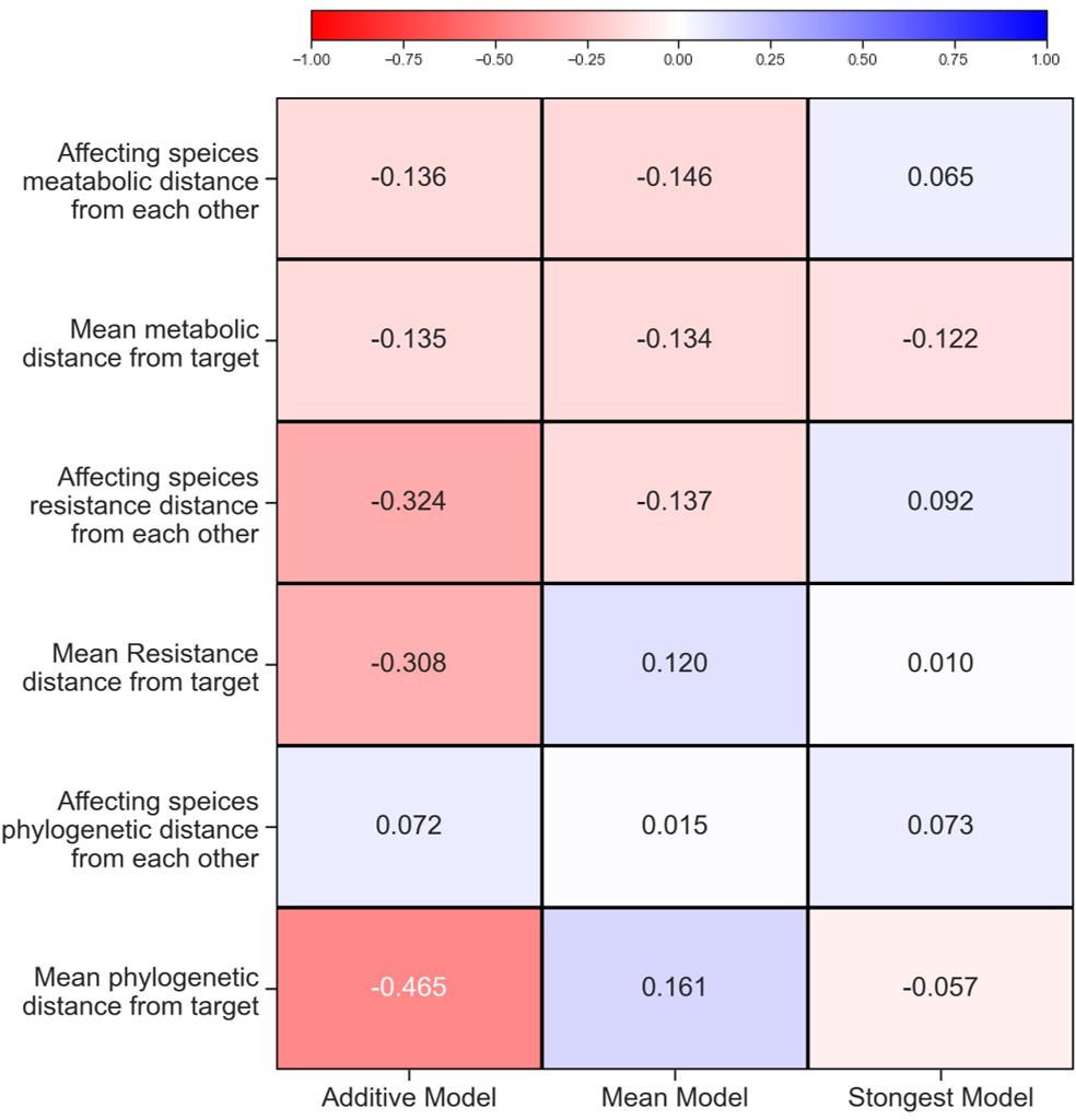
Correlation between affecting species traits and effect on focal.
Spearman correlation value for traits of (A) single species and (B) pairs and effect on species separated for each focal species individually. Correlations with p-values<0.05 are highlighted with a black frame. The growth rate and maximum OD shown in panel (A) were measured only in M9 glucose, similar to conditions used in the interaction assays. See ‘Materials and methods’ for calculations of phenotypic and phylogenetic distances.
Figure 3—figure supplement 2
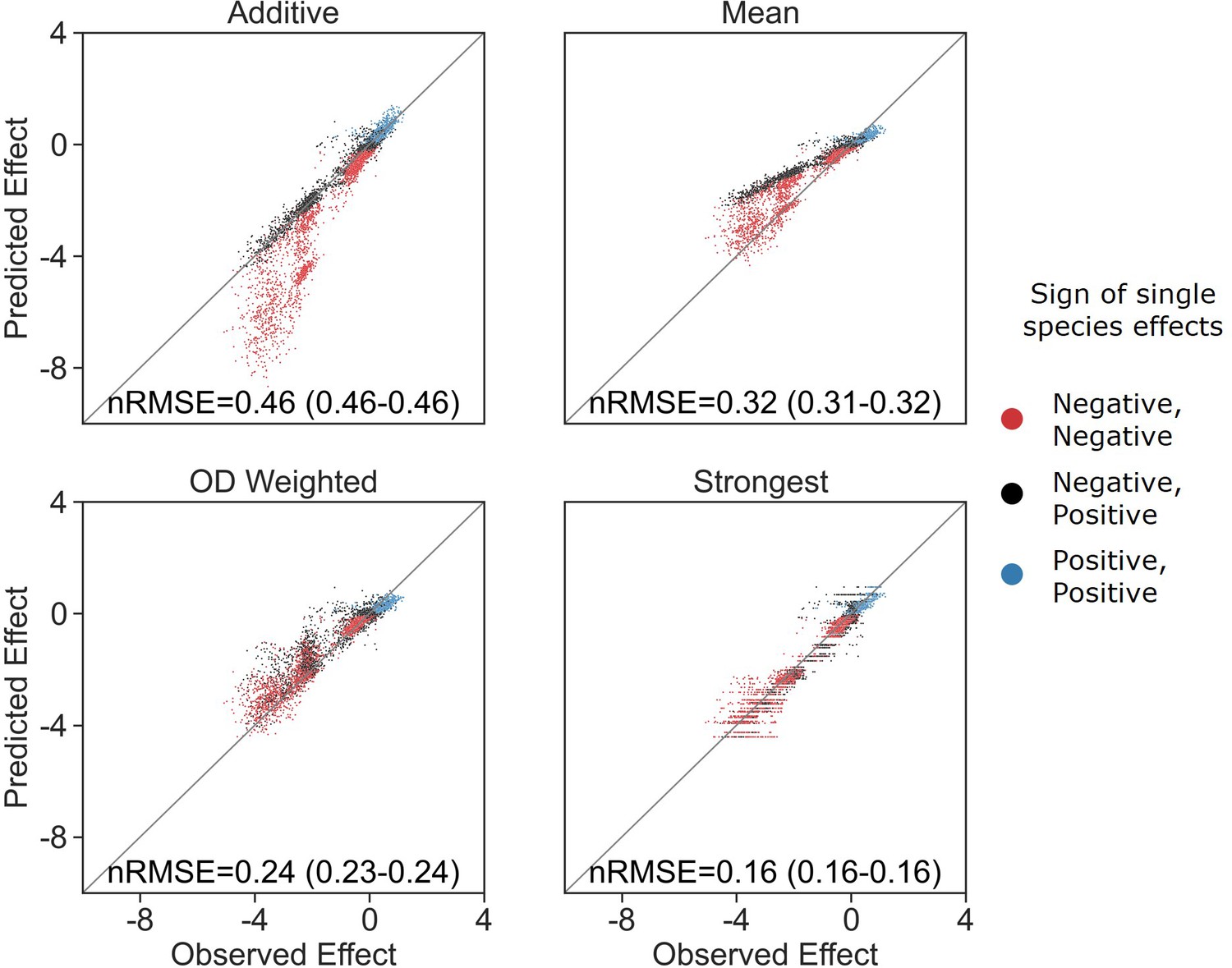
OD-weighted mean model.
Correlation between four different models for how single-species effects combine into pair effects and the experimental data, with their respective normalized root mean squared error (nRMSE). nRMSE values are calculated from 1000 bootstrapped datasets and represent the median and interquartile range in parentheses (see ‘Materials and methods’). Similar to Figure 3B with the addition of the OD-weighted mean.
Figure 3—figure supplement 3
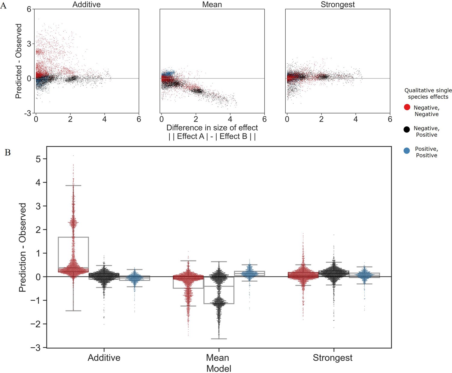
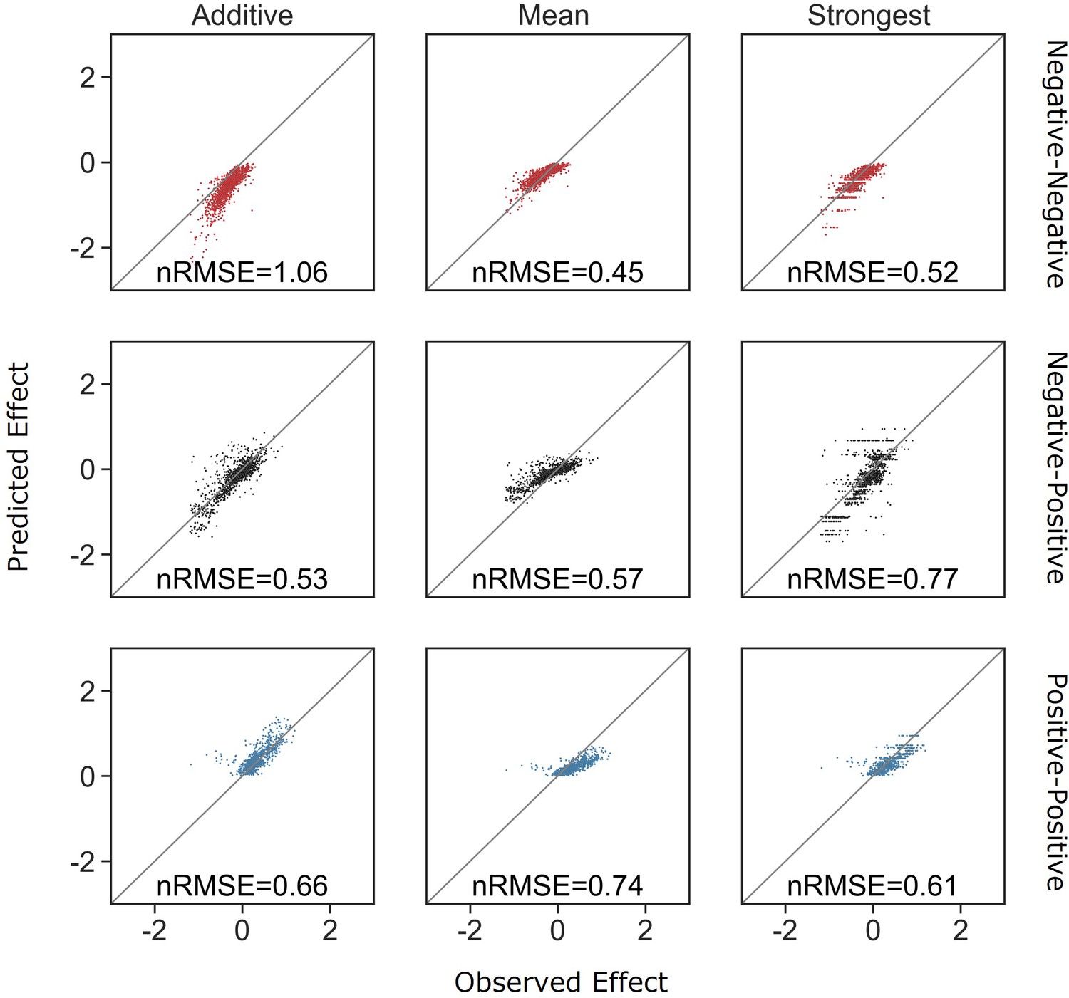
Distribution of errors for each model predicting pair effects from single species.
(A) The accuracy of each model as a function of the difference between the sizes of effect of each individual species within the pair. (B) Distribution of the prediction accuracy for each model. Dots represent individual measurements, solid lines represent the median, boxes represent the interquartile range, and whiskers are expanded to include values no further than 1.5× interquartile range. The frequencies of these interaction types in the dataset are negative–negative 48%, positive–positive 14%, and negative–positive 38%.
Figure 3—figure supplement 4
Traits effect on model error.
Pearson correlation value for each trait and the deviation of the model. Correlations with p-values<0.05 are highlighted with a black frame. See ‘Materials and methods’ for calculations of phenotypic and phylogenetic distances.
Figure 3—figure supplement 5
Accuracy of all models is reduced when considering only combinations of strains that have weak effects.
Correlation between the different models for how single-species effects combine into pair effects, and the experimental data, with their respective normalized root mean squared error. Negative effects and mixed effects were limited to pairs with a combined effect no stronger than –1.2 (the maximum positive effect observed). As the negative–negative and negative–positive predictions become less accurate with these datasets, we posit part of the reason positive–positive interactions were difficult to predict is due to their small effect size.
Figure 3—figure supplement 6
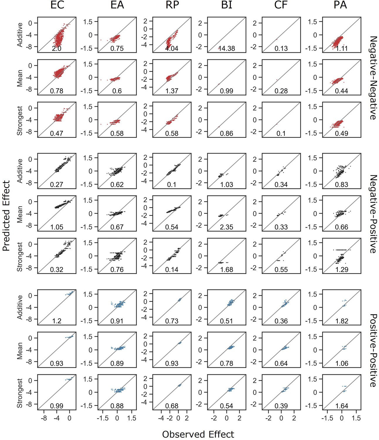
Model comparisons stratified by focal species and interaction type.
Correlation between the different models for how single-species effects combine, and the experimental data, with their respective normalized root squared mean error. Data is divided for each focal species and interaction type individually.
Figure 4 with 1 supplement
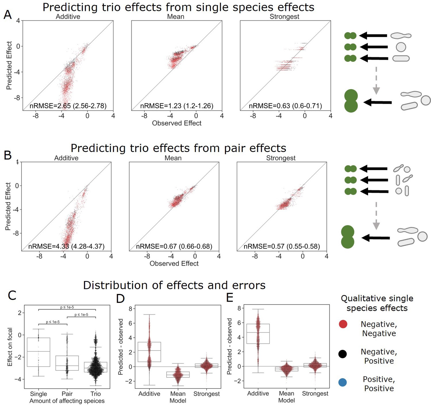
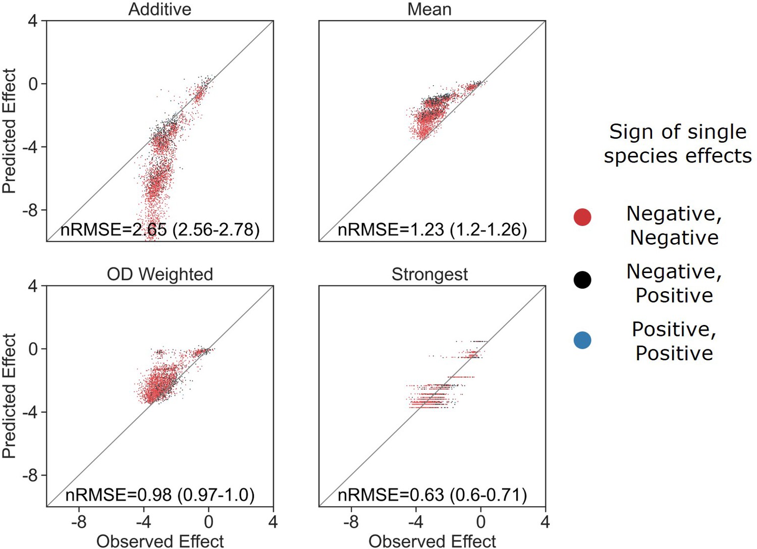
The strongest effect model is also the most accurate for trios.
(A, B) Correlation between three different models for how (A) single-species effects and (B) pairwise species effects combine into trio effects, and the experimental data. Root squared mean error normalized (nRMSE) to the interquartile range. nRMSE values are calculated from 1000 datasets and represent the median and interquartile range in parentheses (see ‘Materials and methods’). (C) Distribution of the effects of single, pairs, and trios of affecting species on E. coli. All Mann–Whitney–Wilcoxon two-sided tests were significant, p values are shown on plot. Dots show individual effects, solid lines represent the median, boxes represent the interquartile range, and whiskers are expanded to include values no further than 1.5× interquartile range. (D, E) Distribution of errors for each model based on (D) single-species data and (E) pairs data. Dots show individual effects, solid lines represent the median, boxes represent the interquartile range, and whiskers are expanded to include values no further than 1.5× interquartile range.
Figure 4—figure supplement 1
OD-weighted mean model.
Correlation between four different models for how single-species effects combine into trio effects and the experimental data, with their respective normalized root mean squared error (nRMSE). nRMSE values are calculated from 1000 bootstrapped datasets and represent the median and interquartile range in parentheses (see ‘Materials and methods’). Similar to Figure 4A with the addition of the OD-weighted mean.
Appendix 1—figure 1
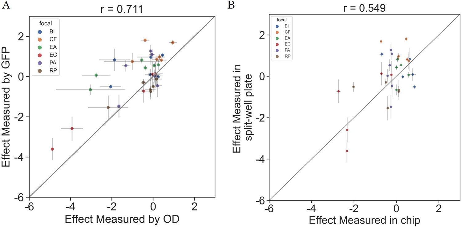
Interactions measured with OD600 are consistent with those based on fluorescent measurements.
The effects of six single species on each focal were measured using OD600 and fluorescence in a 96 split well plate (see ‘Materials and methods’). (A) The correlation between the effect when measured by fluorescence and OD600 (p=1e-6). (B) The correlation between the effect when measured in the kChip and the HTD Equilibrium Dialysis System (p=0.001). Each point represents the median effect of three techinacal repliactes, and error bars represent the standard error calculated viabootstraping (see ‘Materials and methods’).
Appendix 1—figure 2
Model predictions limited by the lowest observed effect.
Correlation between three different models for how single species effects combine, and the experimental data, with their respective normalized root squared mean error. Model predictions were limited to the minimal observed effects, and only data for negative predictions are shown.
Appendix 1—figure 3
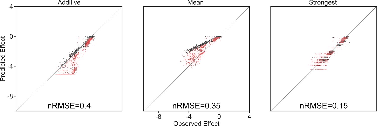
Different models prediction accuracy using all measured effects, not filtered for affecting species autofluorescence.
Correlation between three different models for how (A) single-species effects combine to pairs, (B) single-species effects combine into trio effects, and (C) pairwise species effects combine into trio effects, and the experimental data. Root squared mean error normalized (nRMSE) to the interquartile range. nRMSE values are calculated from 1000 datasets and represent the median and interquartile range in parentheses (see ‘Materials and methods’).
Author response image 1
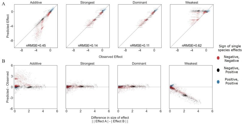
Exploring additional prediction models including weakest effect and dominant effect.
(A) Correlation between four different models for how single species effects combine into pair effects and the experimental data, with their respective normalized root mean squared error. As previously described, the additive model assumes that the effects of each species will accumulate. The strongest effect model assumes that whichever species had a stronger effect on its own will determine the joint effect when paired with an additional species. By contrast The weakest effect model assumes that whichever species had a weaker effect on its own will determine the joint effect when paired with an additional species. The dominant model uses whichever single species effect is closer to the combined effect as it's prediction. (B) The accuracy of each model as a function of the difference between the sizes of effect of each individual species within the pair (similar to Figure 3C from main text).
Additional files
-
MDAR checklist
- https://cdn.elifesciences.org/articles/83398/elife-83398-mdarchecklist1-v2.pdf
-
Source data 1
This file contains the following information regarding the strains in this study: Phylum, Class, Order, Family, and Genus, Nearest species (assigned using BLAST), whether species was used in the trios experiment, Identifier (a taxonomic name for each strain based on the nearest species), 16s rRNA sequences, Genebank accession number for strains isolated in this study.
- https://cdn.elifesciences.org/articles/83398/elife-83398-data1-v2.xlsx
-
Supplementary file 1
This file contains two supplementary tables: the strains used in this study (further details can be found in Source data 1) and the carbon sources and antibiotics (including concentrations) used for phenotypic characterization of the strains.
- https://cdn.elifesciences.org/articles/83398/elife-83398-supp1-v2.docx
Download links
A two-part list of links to download the article, or parts of the article, in various formats.
Downloads (link to download the article as PDF)
Open citations (links to open the citations from this article in various online reference manager services)
Cite this article (links to download the citations from this article in formats compatible with various reference manager tools)
Competitive interactions between culturable bacteria are highly non-additive
eLife 12:e83398.
https://doi.org/10.7554/eLife.83398


