Cryo-plasma FIB/SEM volume imaging of biological specimens
- Structural Biology, Rosalind Franklin Institute, United Kingdom
- Division of Structural Biology, Wellcome Centre for Human Genetics, University of Oxford, United Kingdom
- Artificial Intelligence and Informatics, Rosalind Franklin Institute, United Kingdom
- Diamond Light Source, Harwell Science & Innovation Campus, United Kingdom
- Research Group Cryo-EM Technology, Max Planck Institute of Biochemistry, Germany
- Materials and Structural Analysis Division, Thermo Fisher Scientific, Netherlands
Figures
Figure 1 with 5 supplements

The curtaining score (higher is greater [worse] curtaining) for the different plasma sources at different currents.
Plunge-frozen Chlamydia trachomatis-infected HeLa cells were milled for each current and each gas. 15 windows of 2 × 2.5 × 2 μm3 were milled at different measured currents at 30 kV acceleration voltage for xenon, oxygen, and nitrogen and 20 kV for argon gas (see Figure 1—figure supplements 2 and 3). The incidence angle of the plasma was 18°. SEM images were acquired 90° to the focussed ion beam (FIB). (A) Representative images from these data, showing little or no curtaining (left, oxygen, 213 pA) and extensive curtaining (right, nitrogen, 2.2 nA) seen as vertical lines. Arrow and curly brackets indicate the position of a curtain or group of curtains. Scale bar: 1 μm. (B) Plot of curtaining score as a function of current (see Materials and methods). Points represent the mean value associated with the standard error. The solid line represents the trend across the datapoints. n=15 per condition. (C) Representative images of windows generated with oxygen. Arrow and curly brackets as (A). Scale bar: 1 μm.
Figure 1—figure supplement 1
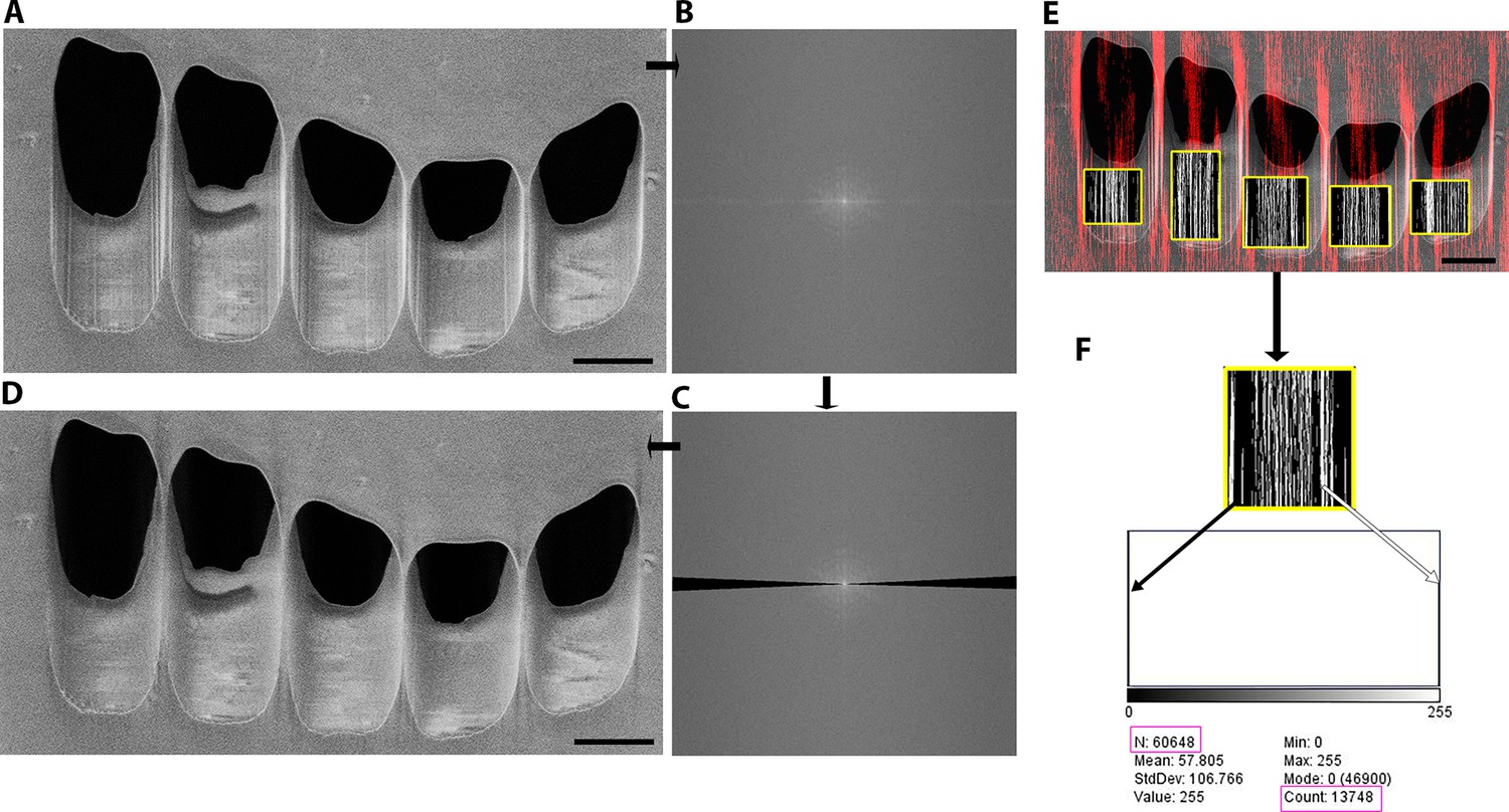
Methods to determine the curtaining score (Materials and methods).
Representative image analysis from HeLa cells milled and imaged using scanning electron microscopy (SEM) at 90° incidence. In this example milling was performed using argon (30 kV, with measured current of 6.1 nA). Using Fiji (Schindelin et al., 2012) an initial image (A) with corresponding FFT (B) was filtered (C) producing a reverse FFT (D) where the vertical lines were removed. Subtracting (D) from (A) produced a mask to isolate the lines and allow the production of a merged image where this mask (red/white) is superimposed onto the initial image (E). From this we can precisely identify the location of the milled window. This allowed the isolation of the area within the mask and determinion of the number of pixels that are part of the curtaining effect using the histogram (F), where white pixels are part of the curtain, and which are counted. The black pixels are not included as part of the curtaining, and the total number of pixels appears as N. Scale bar: 2 µm.
Figure 1—figure supplement 2
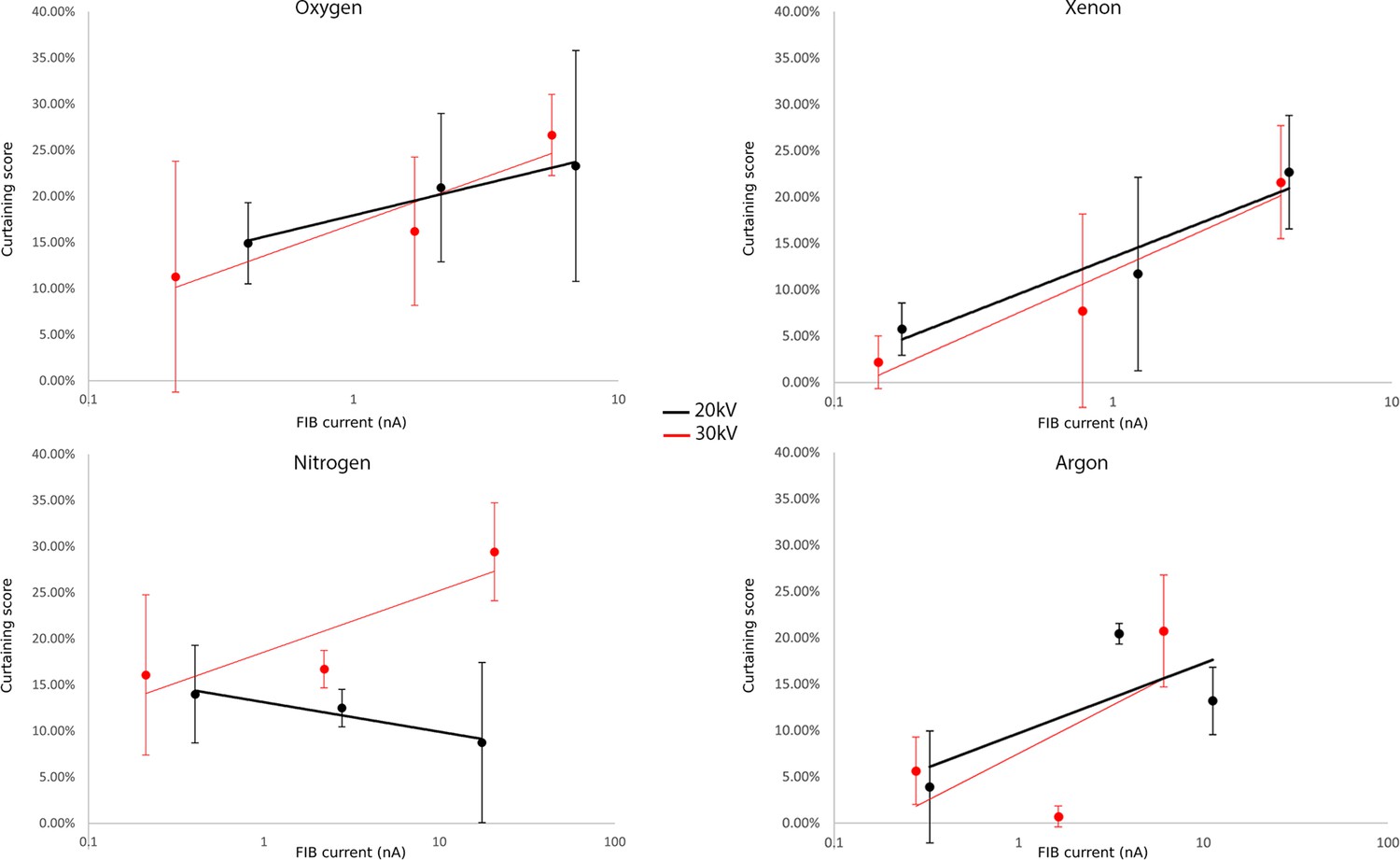
Curtaining score for the different gases at 20 or 30 kV.
Plunge frozen C. trachomatis-infected HeLa cells were milled for the indicated currents for each gas. Fifteen windows of 2 × 2.5 × 2 μm3 were milled at different measured currents at the different acceleration voltages: 30 kV (red) or 20 kV (black). The incidence angle is 18°. Scanning electron microscopy (SEM) images were acquired 90° to the focussed ion beam (FIB). Plots of curtaining score are shown as a function of current (see Materials and methods). Points represent the mean value associated with the standard error. n=15 per condition.
Figure 1—figure supplement 3
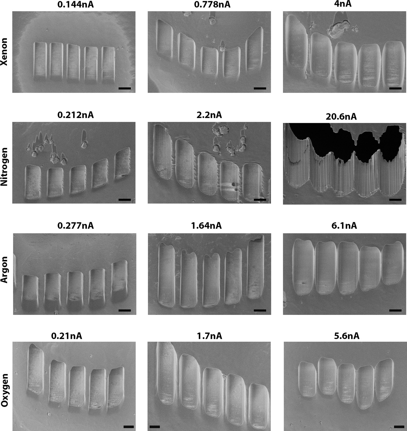
Example of curtaining effects obtained at different current for (top to bottom) xenon, nitrogen, argon, and oxygen, respectively.
Scanning electron microscopy (SEM) images were acquired at 90° incidence. Currents shown are the currents measured on the microscope during acquisition. Scale bar: 2 µm.
Figure 1—figure supplement 4
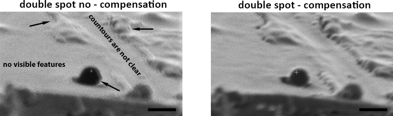
Example of focussed ion beam (FIB) images acquired using nitrogen as ion source with (left) or without (right) double image compensation.
Arrows show where the lines are doubled. Overall contours are unclear and small features are not visible. Scale bars: 1 µm.
Figure 1—figure supplement 5
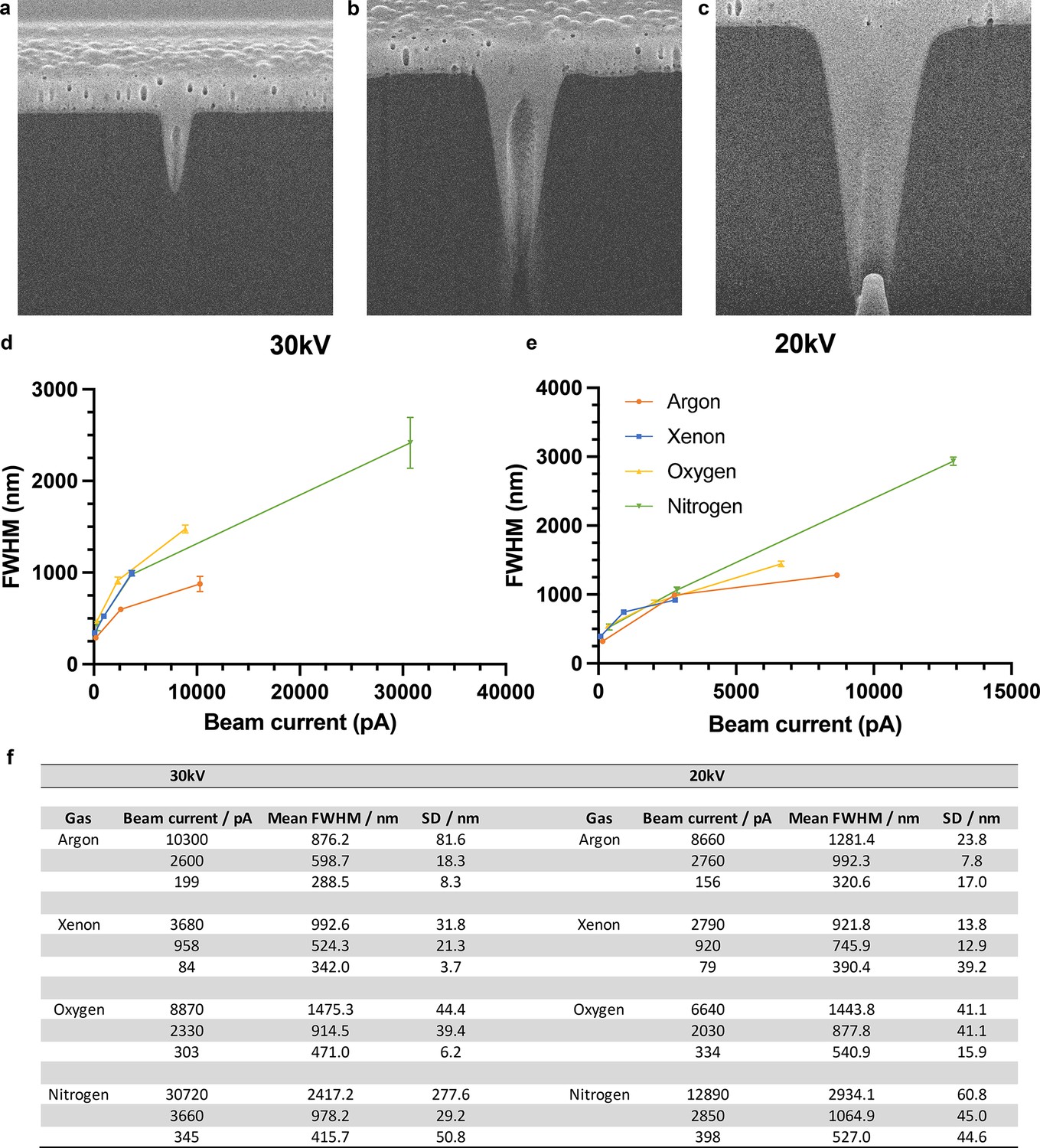
Beam profile characterisation.
Spot burns in silicon (darker contrast) filled with platinum (lighter contrast) were used to observe the beam profile and measure the full width half maximum (FWHM) of three commonly used beam currents covering high, medium, and low currents at both 30 and 20 kV. Argon spot burns at 30 kV are shown for the 200 pA (a), 2nA (b), and 7.6nA (c) apertures. The horizontal field width shown in a–c is 4 µm. The measured FWHMs for all four plasma sources are plotted against the measured beam currents in (d) and (e). Four spot burns were measured and averaged for each gas and beam current, giving a mean FWHM and standard deviation (SD). All measurements are shown in the table (f). The error bars shown in (d) and (e) are the SD from the four measurements. Source data are provided for tables included in this figure. n=2 per conditions.
-
Figure 1—figure supplement 5—source data 1
Data provided for table in Figure 1—figure supplement 5.
- https://cdn.elifesciences.org/articles/83623/elife-83623-fig1-figsupp5-data1-v2.xlsx
Figure 2 with 1 supplement

HeLa cells imaged using serial plasma focussed ion beam (pFIB)/scanning electron microscopy (SEM).
(A–E) Serial pFIB/SEM volume acquired of a HeLa cell, using argon for milling imaged 52° to the surface by SEM. (A) A zoomed-in region of interest, showing nuclear pore complexes (NPCs, arrows) and endoplasmic reticulum (ER). (B) Overview where nucleus, mitochondria (mito), multivesicular body (MVB) and centriole (red box) are easily identifiable. (C) Zoom of the centriole identified in (B) with its three-dimensional (3D) rendering in (D). (E) This HeLa cell presented two centrosomes with two pairs of centrioles and associated pericentriolar matrix (PCM). The distance in green is between the two centrosomes respective centres and the distance in yellow depicts the distance between the centrioles in each pair. (A–C) Slices were filtered using a 2-pixel radius mean filter in Fiji (Schindelin et al., 2012). For (E) we used a band pass filter, also in Fiji. Full data are shown in Figure 2—video 1.
Figure 2—video 1
Volume from serial plasma focussed ion beam (pFIB)/scanning electron microscopy (SEM) of HeLa cells after alignment, Gaussian filtering, and cropping to the region of interest.
Figure 3 with 1 supplement

Non-fixed, high-pressure freezing (HPF) vibratome slice from a mouse brain milled using argon and scanning electron microscopy (SEM) imaging in default configuration (52° to the surface).
(A) Representative slice of wide field of view of the serial plasma focussed ion beam (pFIB)/SEM volume. Scale bar: 1 µm. Coloured insets show regions of interest within the field of view, including myelin sheaths (yellow), putative nuclear pore complexes (red), and mitochondria (blue). Non-coloured insets show synapse morphologies from different slices. Pre- and post-synaptic cells are shown with light pink and magenta arrows, respectively. Scale bar: 500 nm. (B) Enlarged slices from region of (A) indicated in pink of a region containing a neuronal synapse with slices through Z shown at progressive positions, from left to right. Scale bar: 500 nm. (C) Three-dimensional (3D) volume rendering of the synapse presented in (B) with the pre- (green) and post- (purple) synaptic membranes labelled. The post-synaptic density (red) and pre-synaptic vesicles (yellow) are clearly identifiable. For presentation purposes the presented slices have been filtered using a 2-pixel radius mean filter. Full data are shown in Figure 3—video 1.
Figure 3—video 1
Volume from serial plasma focussed ion beam (pFIB)/scanning electron microscopy (SEM) of live slice of mouse brain after alignment, mean filter, and cropping to the region of interest.
Figure 4 with 4 supplements
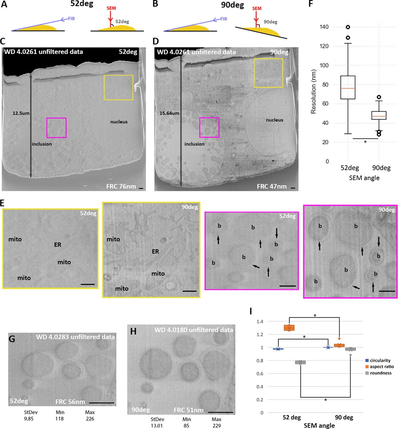
52° vs. 90° Scanning electron microscopy (SEM) imaging angle.
(A) and (B) Schematic of SEM (red arrow) and focussed ion beam (FIB) (purple arrow) angles in default and stage tilt configuration. (A–I) HeLa cells infected with C. trachomatis imaged by serial plasma focused ion beam scanning electron microscopy (pFIB)/SEM using argon to mill. (A–E) Images were acquired using the same parameters except for the tilt angle. No histogram modifications have been made and no filters have been applied. (C) and (D) are the full field of view and (E) zoomed-in panel (colour boxes). Arrows show the outer membrane of bacteria. (F) presents the resolution obtained for the different patches on images acquired at 52° (n=251 patches) or 90°(n=303 patches) to the surface using FRC to measure. (G–H) In addition to the angle, the working distance (WD) was modified while other imaging parameters kept identical. (I) Bacteria (n=8) were segmented for circularity, aspect ratio, and roundness to be calculated (Rueden et al., 2017) and presented in this graph as a function of the imaging angle with the standard deviation. All values were normalised to the case of a perfect circle having a value of 1.0. *Indicates a significant difference (0.1%). WD: working distance, FRC: Fourier ring correlation, mito: mitochondria, ER: endoplasmic reticulum, b: bacteria. Scale bars: 500 nm (C, D and E) and 1 µm (G and H).
Figure 4—figure supplement 1
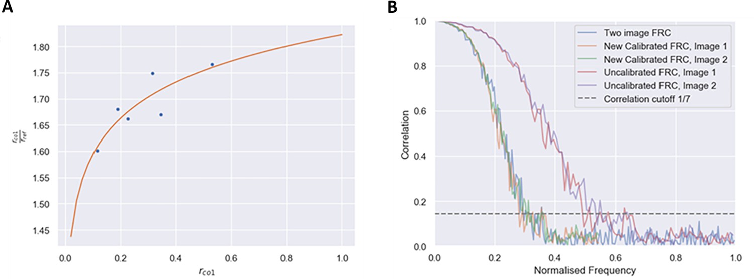
Fourier ring correlation (FRC) evaluation method (Materials and methods).
(A) Calibration curve obtained from the EM calibration dataset. Each point represents a pair of images taken at each pixel size and each scanning electron microscopy (SEM) angle. (B) Application of a calibration factor to the one-image FRC matches the FRC curve to the gold-standard two-image FRC, as shown by the orange and green lines (calibrated one-image FRC) closely following the blue line (gold-standard two-image FRC). The red and purple lines (uncalibrated FRC) do not match the gold standard FRC curve, so the resolution value taken from these curves are incorrect.
Figure 4—figure supplement 2
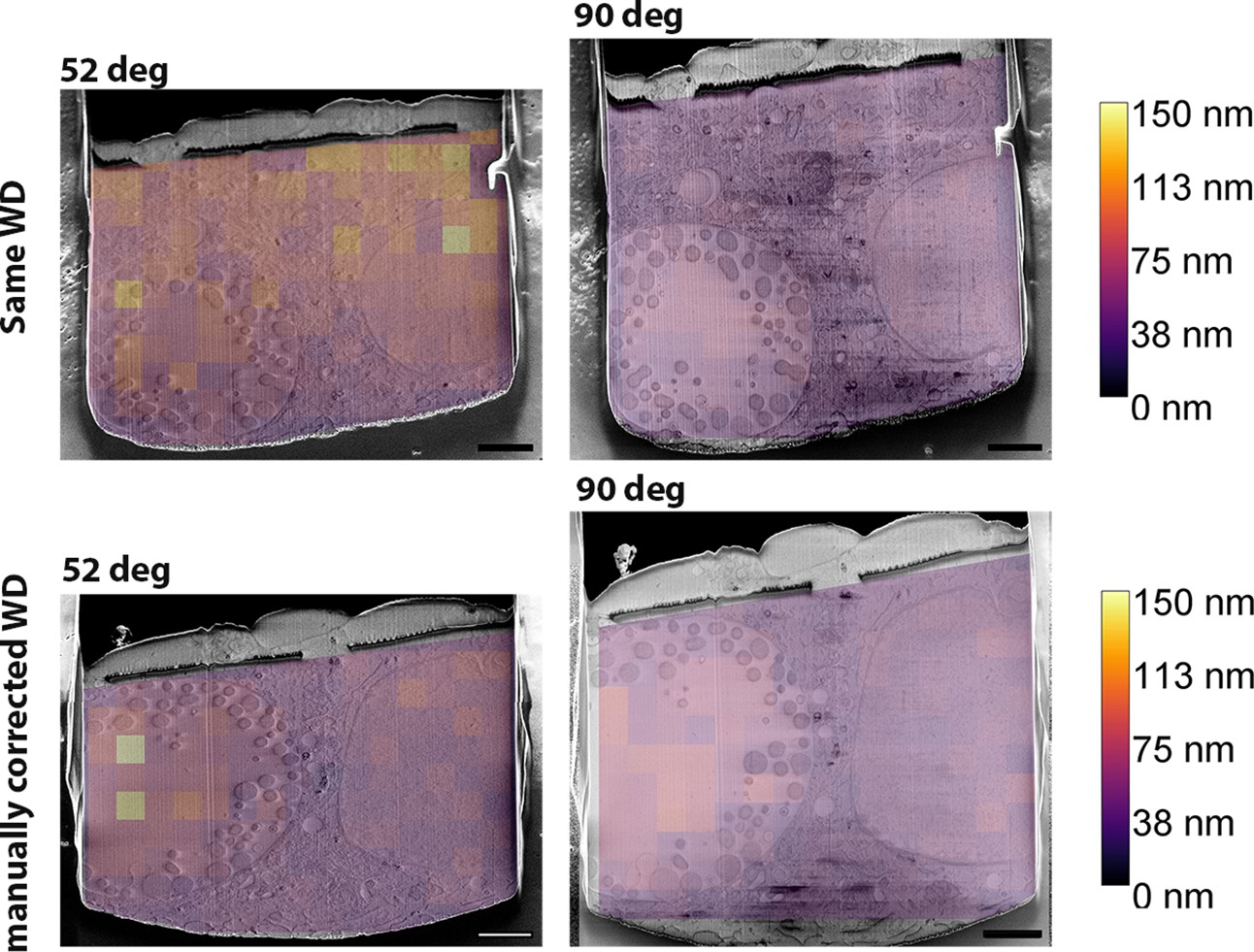
Relationship between resolution and working distance.
Scanning electron microscopy (SEM) images taken at different imaging angles (52° or 90° to the SEM column) are overlaid with the results of the measured Fourier ring correlation resolution (heat map). Results are shown for instances where the working distance (WD) either remains the same (top) or not (bottom), while all the other parameters remain identical. Scale bar: 2 µm.
Figure 4—figure supplement 3
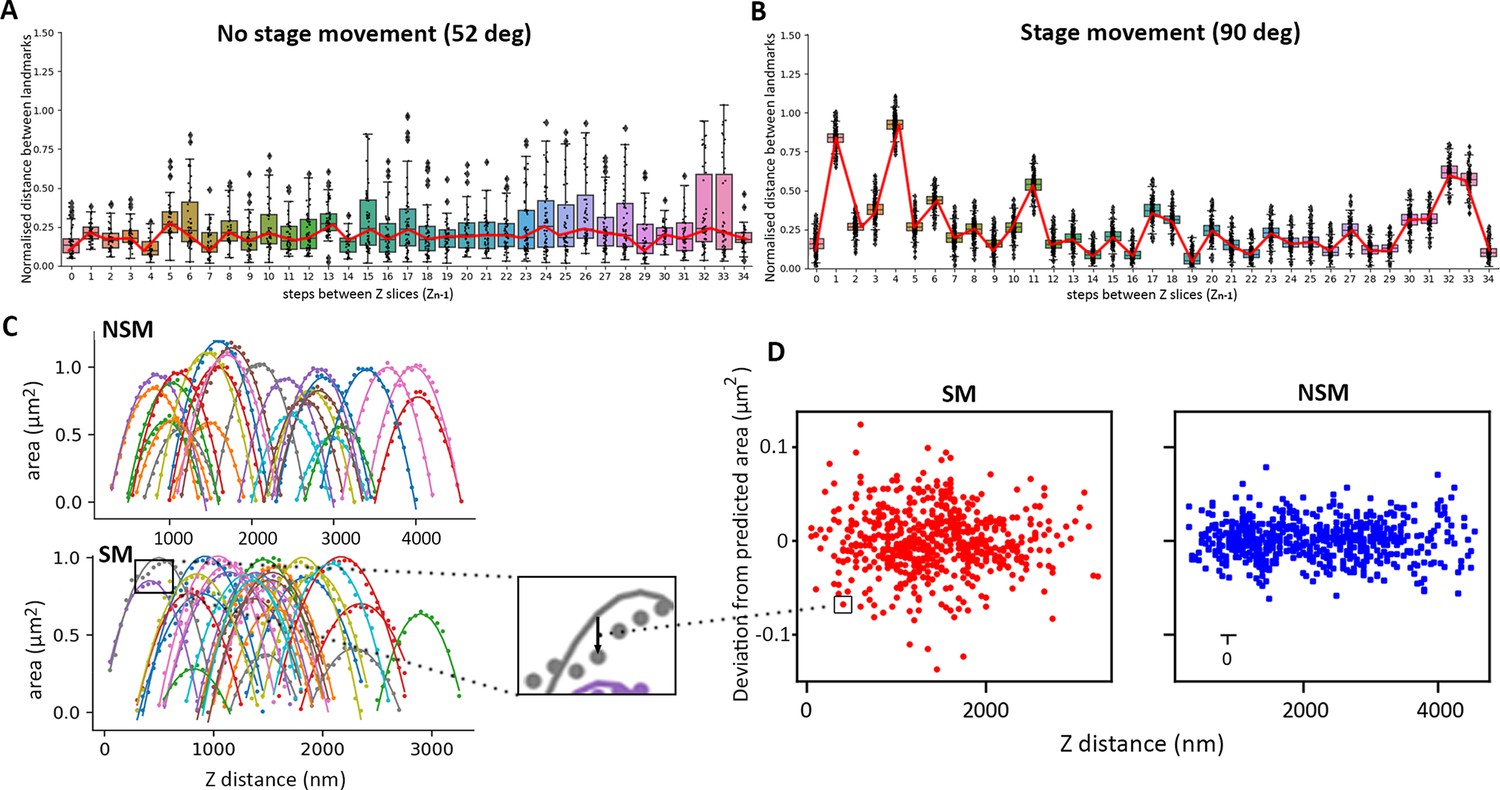
Measurement of XY (A and B) and Z drift (C and D) during data acquisition with no stage movement (NSM) imaged 52° to the scanning electron microscopy (SEM) or with stage movement (SM), imaged 90° to the SEM.
Serial plasma focussed ion beam (pFIB)/SEM stacks of 1 µm PEG beads were acquired with a 50 nm milling step using argon. (A and B) represent the normalised distance between bead landmarks (distance between landmarks/diagonal of the field of view) as a function of the step between slices (Zn−1). Red lines highlight the variation of the average in the position of the landmark (points). No stage movement: n=49/image, Stage movement: n=331/image (C) Individual bead cross-section area as a function of Z position (Z distance in nm, which is the Z slice number multiplied by the target milling thickness, in this case 50 nm). Points display the measured area from the dataset, and the solid line is the optimised curve for a perfect spherical bead. The deviation between prediction and measurement (example in the zoom box highlighted by an arrow) is plotted in (D) (deviation as a function of Z distance).
Figure 4—figure supplement 4

Measurement of depth of field.
A tin ball sample was imaged at different stage position (Δ5 µm) normal to the scanning electron microscopy (SEM) using immersion mode at 1 or 2 kV 12.5 pA. The Fourier ring correlation (FRC) was then calculated and compared stage position by stage position to estimate if it was equal with 5% error (test). By taking the depth of field and measuring where the FRC is constant (t-test 95% confidence marked by an asterix), we can estimate the depth of field to be ~20 µm for imaging both at 1 and 2 kV. n=24.
Figure 5 with 1 supplement
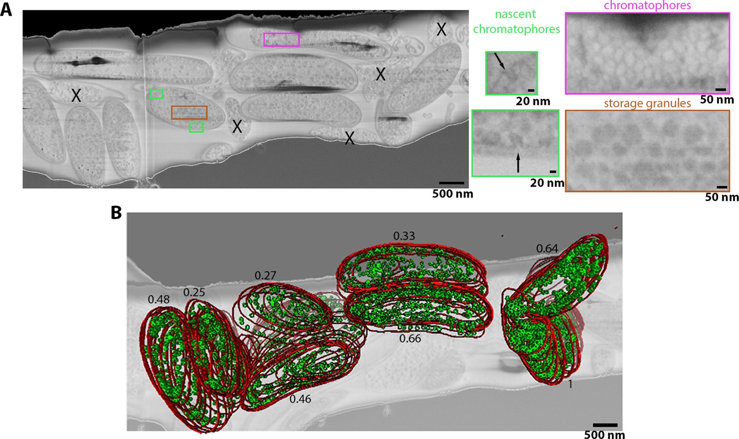
R. rubrum image stacks acquired using argon serial plasma focussed ion beam (pFIB)/scanning electron microscopy (SEM) normal to the SEM column.
(A) Full field of view of slice of serial pFIB/SEM volume, showing vitrified R. rubrum. Features within the bacteria are shown enlarged (right), with highlighted areas showing nascent chromatophores (green), mature chromatophores (pink), and storage granules (brown). X indicates dead/dying bacteria or debris. (B) Slice of the volume superimposed with the volume rendering after segmentation. In red is the outer membrane and green the mature chromatophores. The number associated with each segmented bacteria is the ratio of the number of chromatophores per sum of the surfaces occupied by the bacteria at each slice. The slice was filtered using a 2-pixel radius Gaussian filter. Full data are shown in Figure 5—video 1.
Figure 5—video 1
Volume from serial plasma focussed ion beam (pFIB)/scanning electron microscopy (SEM) of R. rubrum after alignment, mean filter, and cropping to the region of interest.
Figure 6 with 2 supplements

Vero cells imaged using serial plasma focussed ion beam (pFIB)/scanning electron microscopy (SEM) normal to surface.
(A–E) Serial pFIB/SEM volume acquired of a Vero cell, using nitrogen plasma for milling. (A) Field of view (FOV) with insets show enlarged regions of endoplasmic reticulum (ER) and mitochondria with visible cristae (yellow), and enlarged region populated with nuclear pore complexes (blue) (arrows). The vertical curtains on the left of the yellow box in the large FOV image (left) arise from contamination at the surface of the cell. (B) Three-dimensional (3D) segmentation of subcellular features within the volume in (A). Red: lipid droplets (LDs), green: mitochondria, cyan: LD-to-ER membrane contact site (MCS) (max. 25 nm space between the membranes), purple: mitochondria to ER MCS. (C) Number of different ER MCS in contact with organelles vs. the contact volume (µm3), for LDs (blue) and mitochondria (pink). (D) Volume (µm3) of complete mitochondria within the volume of the Vero cell are shown. (E) Volume (µm3) of the FOV and different organelles. Full data are shown in Figure 6—video 1 and full segmentation including ER are available in Figure 6—video 2. Source data are provided for tables included in this figure.
-
Figure 6—source data 1
Data provided for table in Figure 6.
- https://cdn.elifesciences.org/articles/83623/elife-83623-fig6-data1-v2.xlsx
Figure 6—video 1
Volume from serial plasma focussed ion beam (pFIB)/scanning electron microscopy (SEM) of Vero cells after alignment, mean filter, and cropping to the region of interest.
Figure 6—video 2
Segmentation (Amira) from the volume from serial plasma focussed ion beam (pFIB)/scanning electron microscopy (SEM) of Vero cells after alignment, mean filter, and cropping to the region of interest.
Yellow: endoplasmic reticulum, red: lipid droplets, green: mitochondria, cyan: lipid droplets to endoplasmic reticulum (ER) membrane contact sites, purple: mitochondria to endoplasmic reticulum membrane contact sites.
Figure 7 with 1 supplement
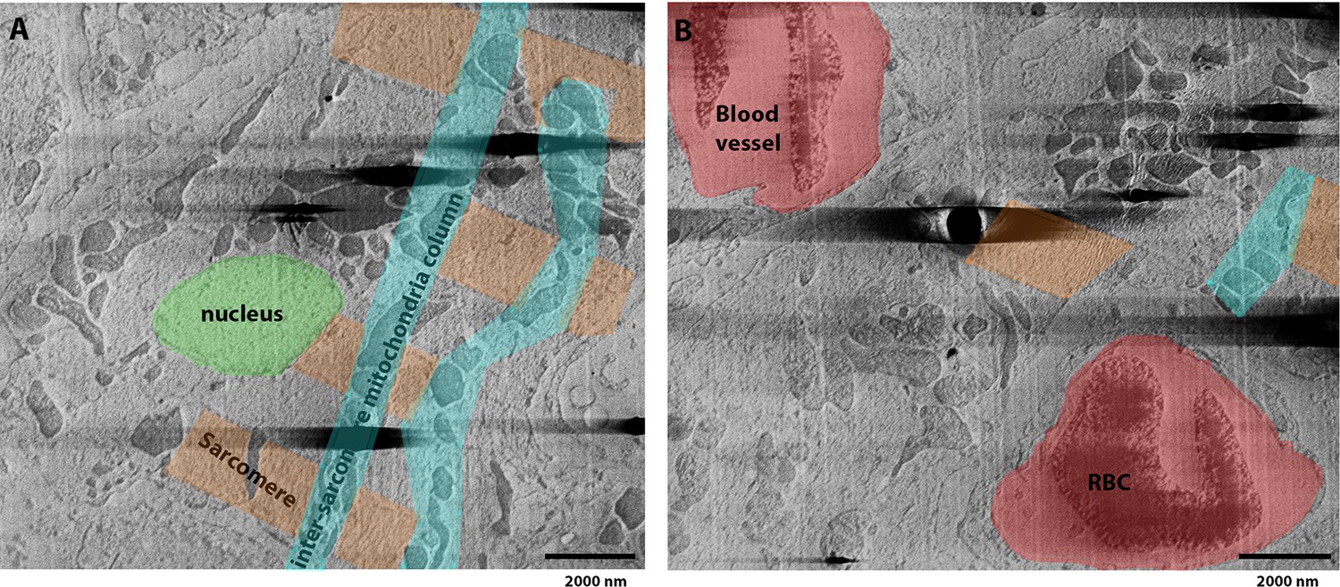
Fixed, high-pressure frozen (HPF) vibratome slice from a mouse heart image milled using argon and imaged normal to the surface.
(A) Slice from serial plasma focussed ion beam (pFIB)/scanning electron microscope (SEM) volume showing subcellular structures consistent with those recognised from a cardiac myofibril (Begay et al., 2018), with a nucleus (green), sarcomeric elements (including Z-disc, I-band, and A-band) (orange), and mitochondria organised between axially organised sarcomeres in columns (cyan). (B) Slice of the tomogram preceding the image shown in (A), where amongst the cardiac tissue, blood vessels and red blood cells (RBC) can be identified (red). Figure 7—video 1 presents the whole data.
Figure 7—video 1
Volume from serial plasma focussed ion beam (pFIB)/scanning electron microscopy (SEM) of fixed slice of mouse heart after alignment, mean filter, and cropping to the region of interest.
Figure 8 with 1 supplement
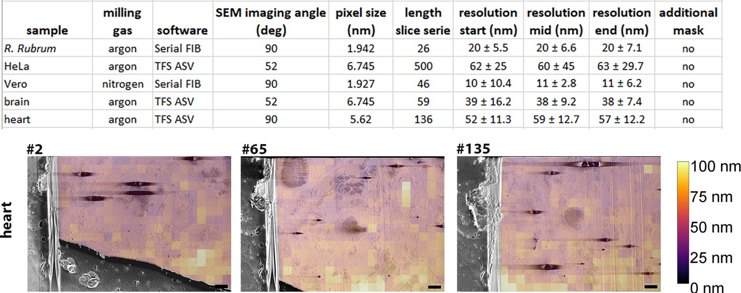
Fourier ring correlation (FRC) resolution measurements for biological samples.
(A) Table presents the acquisition parameters and the associated calculated resolution for the dataset presented in Figures 3—6. The length of the series represents the number of slices. All datasets were acquired using a 50 nm step. FRC resolution measurements were determined using image slices taken from serial plasma focussed ion beam (pFIB)/scanning electron microscope (SEM) volumes - three slices were used (start, mid, end) from each dataset. In all cases, the organoplatinum layer was masked out of these measurements. Software used are either SerialFIB (Klumpe et al., 2021) or Thermo Fisher Scientific Auto Slice and View (TFS ASV). For R. Rubrum the number of patches is n=383, for HeLa n=95, for Vero n = 251, for the brain n = 95 and for the heart n = 301, 383 and 385 for the start, middle and end respectively. (B) Example of the FRC analysis from the heart dataset. Slice numbers 2, 65, and 135 are the one used for start, mid, and end. Scale bars: 2 µm. Figure 8—figure supplement 1: FRC overlays for HeLa, brain, and R. rubrum. Source data are provided for tables included in this figure.
-
Figure 8—source data 1
Data provided for table in Figure 8.
- https://cdn.elifesciences.org/articles/83623/elife-83623-fig8-data1-v2.xlsx
Figure 8—figure supplement 1
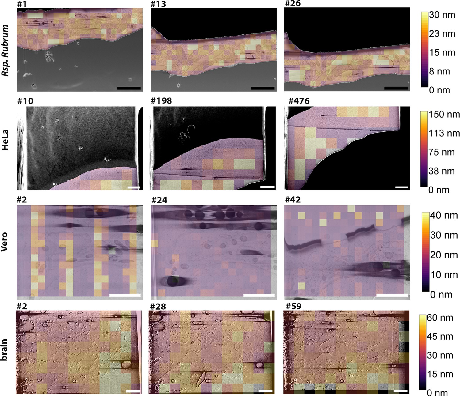
Analysis of the resolution from different biological data acquired at different points during data acquisition (start, middle, end).
Slices from serial plasma focussed ion beam (pFIB)/scanning electron microscopy (SEM) volumes taken at positions towards the beginning of the acquisition (left), at a point in the middle (middle) and towards the end (right). The slice number is shown above the respective images. The colour scheme relates to the locally measured resolution across the field of views using the Fourier ring correlation approach are presented as overlays of the sample and the generated heat map (colour code on the right). Scale bars: 2 µm.
Figure 9 with 5 supplements
Correlation of fluorescence, serial plasma focussed ion beam (pFIB)/scanning electron microscopy (SEM), and transmitted electron microscopy (TEM) at cryogenic temperatures.
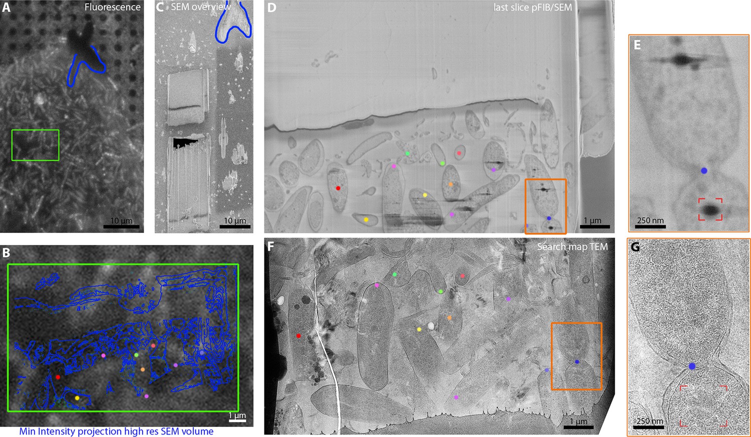
(A and B) R. rubrum were imaged using fluorescence microscopy within the dual-beam microscope chamber before the deposition of the protective platinum layers. Serial pFIB/SEM was then performed (D and E and Figure 9—video 1) and then TEM images of the lamella acquired subsequently (F and G). The coloured dots presented in panels B and D–G are common features between the different imaging modalities. The green rectangles in A and B represent the regions of interest (ROI) where serial pFIB/SEM was acquired. The orange rectangle in D and E highlights the septum on both SEM and TEM while the red corner the presence of lipid droplets in E and G. The blue outline present on (A–C) indicates the outline used to align the fluorescence and SEM images. The images were not filtered.
Figure 9—figure supplement 1

Correlation between plasma focussed ion beam (pFIB)/scanning electron microscopy (SEM) and transmitted electron microscopy (TEM).
Retinal pigment epithelial-1 (RPE-1) hTERT cells were prepared using a combination of serial pFIB/SEM imaging normal to the SEM, using argon 30 kV for milling (A–C). The video acquired during milling was acquired with a slice spacing of 100 nm (Figure 9—video 2). Serial pFIB/SEM was stopped when reaching a defined milling volume. The lamella was then prepared usign a 60 pA current to polish on both sides of the lamella and imaged using a 300 kV TEM. A medium mag montage was acquired to form a search map (D–F). The green and blue rectangles represent sequential zoom-in area, with green dots highlighting common features between the different imaging modalities. The cyan line depicts the plasma membranes for panels A and D, while the red circle the lipid droplets for panels A, C, D, and F, and the yellow circle in C and F a compartment in close proximity to the lipid droplet. All images are unfiltered.
Figure 9—figure supplement 2
Correlation between serial plasma focussed ion beam (pFIB)/scanning electron microscopy (SEM) and cryo-electron tomography.
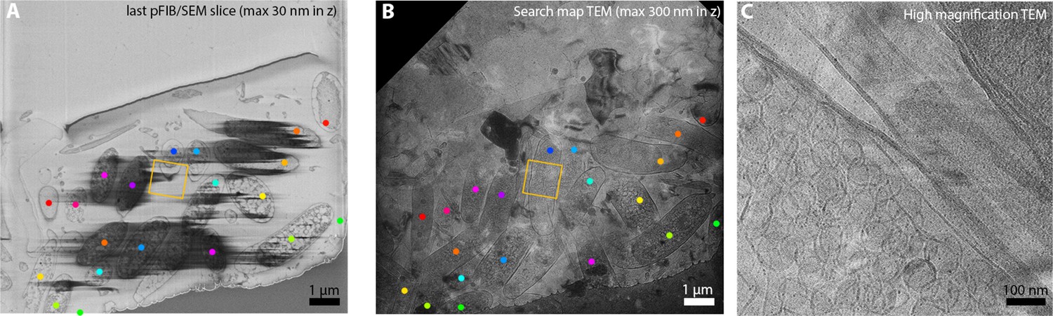
R. rubrum was imaged using serial pFIB/SEM (Figure 9—video 3) using argon for milling and imaging the normal to the SEM (A). The sample was then transferred to the transmitted electron microscopy (TEM) to acquire a TEM intermediate magnification (B) followed by a high magnification tomogram (C). The dots represent common features between the SEM and TEM, apart from the bright green dots which mark an absence of features in the SEM. The orange rectangle designates the location for the acquisition of the tilt series. (A) and (B) are raw images and (C) were filtered using a mean 2-pixel filter in Fiji (Schindelin et al., 2012).
Figure 9—video 1
Volume from serial plasma focussed ion beam (pFIB)/scanning electron microscopy (SEM) of fixed slice of of R. rubrum after alignment and cropping to the region of interest.
Figure 9—video 2
Volume from serial plasma focussed ion beam (pFIB)/scanning electron microscopy (SEM) of fixed slice of of retinal pigment epithelial-1 (RPE-1) cells after alignment and cropping to the region of interest.
Figure 9—video 3
Volume from serial plasma focussed ion beam (pFIB)/scanning electron microscopy (SEM) of fixed slice of of R. rubrum after alignment and cropping to the region of interest.
Figure 10

Post-processing computational approach to mitigate charging artefacts.
Cells were imaged normal (90°) to the surface and argon used for milling. (A) Depiction of the results of instance segmentation of lipid droplets found within the serial plasma focussed ion beam (pFIB)/scanning electron microscopy (SEM) volume. The lipid droplet highlighted in the yellow box in (A) is shown inset (B) with the same region shown in (C) after charging artefact suppression. The inset (D) shows the charging artefacts in isolation and demonstrates their asymmetry – this is produced when (C) is subtracted from (B). Since the artefact is asymmetric, different functions were fitted on the left and right of the charging artefacts. (E) and (F) are vertical and horizontal grey value line profiles through the lipid droplet in (B) and (C), respectively. (G) aggregated vertical and horizontal line profiles for 20 lipid droplets from (A) show that filtering to remove charging artefacts restores the sharp dip in grey values for the lipid droplets in the horizontal line profile, and more closely matches the grey values on either side of the charging centre, as can be seen in the vertical line profiles (Pennington et al., 2022).
Figure 11

Automated segmentation of subcellular features using SuRVoS2.
(A) A representative XY slice from the serial plasma focussed ion beam (pFIB)-scanning electron microscopy (SEM) of heart tissue data. (B) The same SEM image overlaid with the automated segmentation produced by SurVoS2 after training a multi-axis U-Net++ (orange). Artefacts such as lipid droplets are masked out of the segmentation (green). A section of the serial pFIB/SEM data was used to compare the manual segmentation of mitochondria vs. SuRVoS2 segmentation (red box). For A and B, scale bar = 1.2 µm. (C) Evaluation of the automated segmentation output from SuRVoS2. A 128 × 128 × 128 region within the top right quadrant of the serial pFIB/SEM data was extracted (C i–iii) and the mitochondria within XY slices were segmented manually to establish a ‘ground truth’ (D i–iii). The trained multi-axis U-Net++ network then automatically segmented the region (E i–iii). The Dice score between the segmentation and ground truth is 0.87, with the qualitative performance of the segmentation increasing in accuracy from left to right. In the less accurate automated segmentations, changes in contrast due to charging were erroneously segmented (left column, red arrows). Small regions within mitochondria are not segmented (E ii, yellow arrow) whilst some small regions that are not part of a mitochondria are segmented incorrectly (E ii–iii, green arrows). Scale bar: 250 nm.
Author response image 1
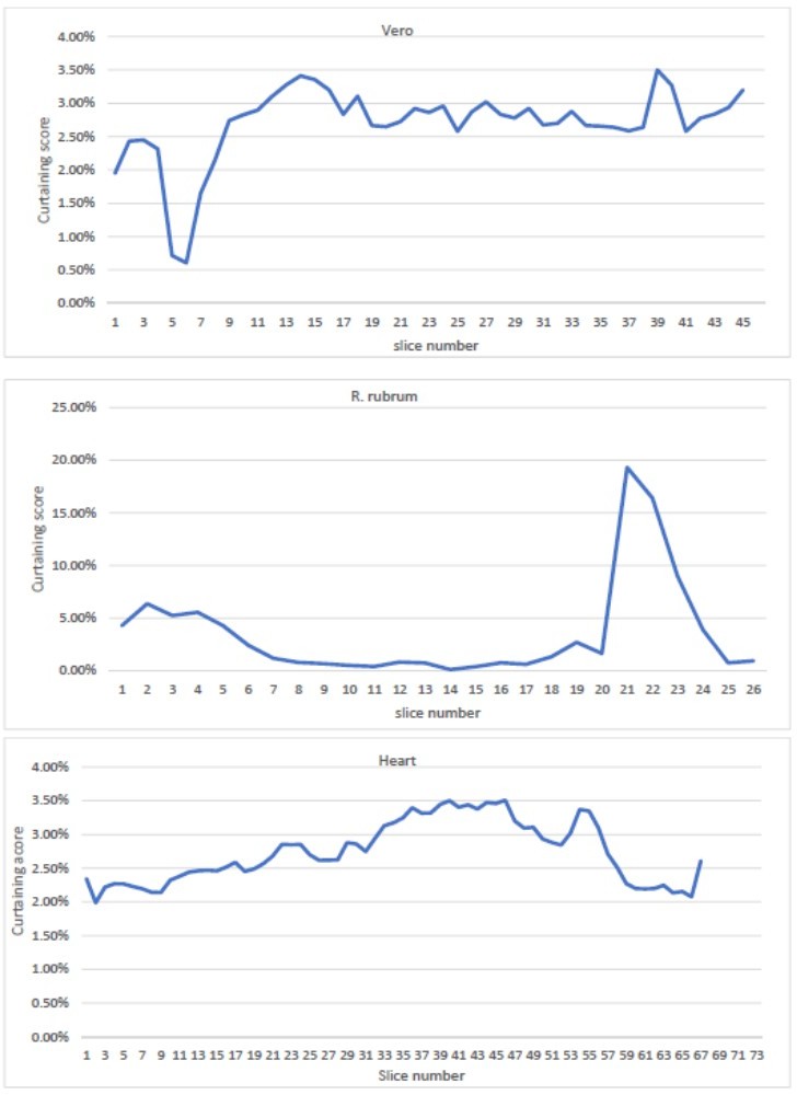
Curtaining rate from the mouse heart, Vero cells and R.
rubrum raw dataset as a function of slice number.
Author response image 2
Tables
Table 1
Serial plasma focussed ion beam (pFIB)/scanning electron microscope (SEM) parameters used for the different biological samples.
| Sample | Milling gas | Acceleration voltage (kV) | Target current (nA) | Software | SEM imaging angle (°) | Pixel size (nm) | SEM voltage (kV) | SEM current (pA) | Dwell time (ns) | Line integration | Gain (%) | Offset voltage (V) | Electron dose (e−/A2) |
|---|---|---|---|---|---|---|---|---|---|---|---|---|---|
| HeLa | Argon | 20 | 0.2 | TFS ASV | 52 | 6.745 | 1.25 | 6.25 | 100 | 100 | 62.9 | –12 | 8.24×10⁻⁴ |
| Vero | Nitrogen | 30 | 0.27 | Serial FIB | 90 | 1.927 | 1.2 | 6.25 | 100 | 100 | 56.45 | –8.4 | 9.84×10⁻³ |
| Rubrum | Argon | 20 | 0.2 | Serial FIB | 90 | 1.942 | 1.1 | 6.25 | 100 | 100 | 36 | –3.37 | 9.94×10⁻³ |
| Brain | Argon | 20 | 0.2 | TFS ASV | 52 | 6.745 | 1.1 | 6.25 | 500 | 16 | 40.25 | –4.37 | 8.24×10⁻⁴ |
| Heart | Argon | 20 | 0.2 | TFS ASV | 90 | 5.62 | 1.1 | 6.25 | 100 | 100 | 45.42 | –4.41 | 1.19×10⁻⁴ |
-
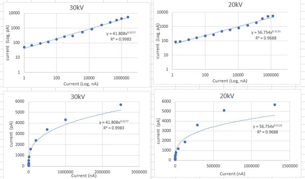
Formula from current measured using Faraday cup.
Table 2
Focussed ion beam (FIB) current (targeted value) in nA.
| Argon | Xenon | Nitrogen | Oxygen | |
|---|---|---|---|---|
| 20 kV | 6.2 | 3.3 | 14 | 4.2 |
| 2.4 | 1 | 1.8 | 1.4 | |
| 0.2 | 0.1 | 0.32 | 0.29 | |
| 30 kV | 7.6 | 4 | 24 | 5.6 |
| 2 | 1 | 1.7 | 1.7 | |
| 0.2 | 0.1 | 0.27 | 0.23 |
Additional files
Download links
A two-part list of links to download the article, or parts of the article, in various formats.
Downloads (link to download the article as PDF)
Open citations (links to open the citations from this article in various online reference manager services)
Cite this article (links to download the citations from this article in formats compatible with various reference manager tools)
Cryo-plasma FIB/SEM volume imaging of biological specimens
eLife 12:e83623.
https://doi.org/10.7554/eLife.83623


