Metabolic model-based ecological modeling for probiotic design
Figures
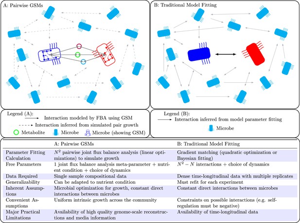
Population models such as Lotka-Volterra generally require dense time-longitudinal data to accurately parameterize, and directly fit interactions between species (solid arrow in right panel).
In this work, we leverage genome-scale metabolic modeling to parameterize population models with only genomic data from a single time-point. This is accomplished by modeling microbial interactions with their shared environment (colored circles in the left panel).
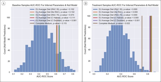
Comparison of AUC-ROC Between Inferred Parameters & Null Model.
(A, B) The power to predict engraftment versus non-engraftment of the B. longum probiotic was relatively robust to the joint flux balance analysis (FBA) hyperparameter setup, as shown and measured by the area under the receiver operator characteristic curve (AUC-ROC) (with 1 being perfect classification of engraftment and 0.5 being random). The null model had generally less predictive power than inferred parameters, in particular when predictions were made with samples from the ‘treatment’ time-point. The overall improvement in predictions for the ‘treatment’ time-point vs. the ‘baseline’ time-point suggests that early changes to the microbiome after introduction of a probiotic play a significant role in determining eventual engraftment. p-Values were estimated based on over 1000 samples from a null model.
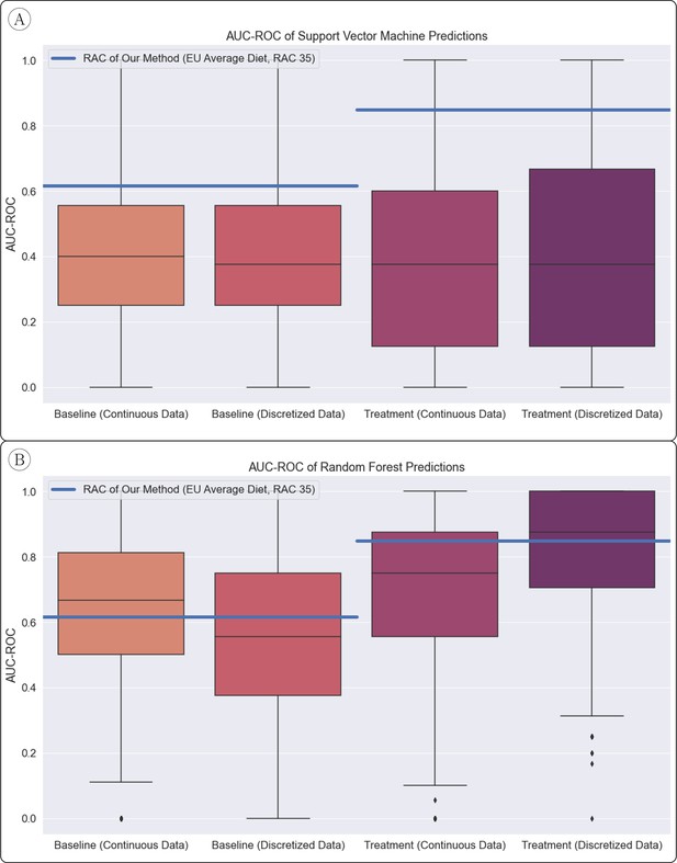
AUC-ROC of Standard Classifier Predictions.
(A) Our method (horizontal lines) significantly outperformed the support vector machine classifier, which was assessed with 1000 random train/test splits. (B) The random forest classifier, also assessed with 1000 train/test splits, performed similarly on average to our method.
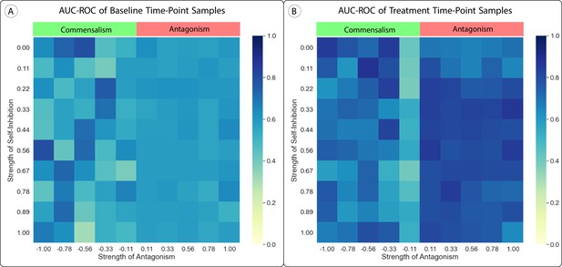
Effect of Uniform Parameter Shifts in the Lotka-Volterra Model.
(A, B) We altered the generalized Lotka-Volterra model with uniform shifts in parameters which added either antagonism or self-inhibition to the model. We tested self-inhibition with values from 0 to 1 (no self-promotion) and antagonism with values from 1 (complete antagonism) to –1 (complete commensalism), with all . Neither change had a significant impact on the area under the receiver operator characteristic curve (AUC-ROC) of our method’s predictions, although adding commensalism to the model made the model and resulting predictions much less stable due to increased finite-time blow-up.
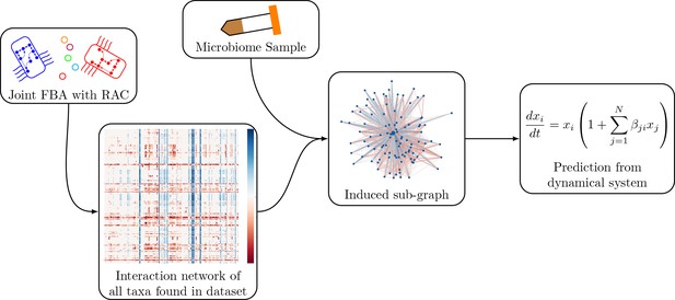
Schematic of the modeling process.
In brief, we generate an interaction network of genome-scale models using pairwise joint flux balance analysis. To produce a prediction of engraftment for a given sample, we use the taxa present in the sample to generate an induced sub-graph of the full network. This is then used to define the parameters in the generalized Lotka-Volterra dynamical system to generate a prediction of engraftment.
Tables
Area under the receiver operating characteristic curves for our method’s predictions of 22 samples from each of two time-points (TP) using six sets of parameters inferred from joint flux balance analysis (FBA) with six different sets of hyperparameters.
The first three sets of inferred parameters differ in the ‘resource allocation constraint (RAC)’ in joint FBA. We used values of 35 and 70 for this parameter, as well as using joint FBA without RAC. The next three sets of parameters were inferred using an RAC value of 35 but changes to the model environments. EU average diet (C halved/doubled) had the major carbon sources of the ‘EU average diet’ (D-maltose, sucrose, D-fructose, and D-glucose) halved or doubled in availability, and ‘complete medium’ simulated the availability of any exchangeable metabolite at uniform simulated inflow.
| Baseline TP (p-value) | Treatment TP (p-value) | |
|---|---|---|
| EU average diet (RAC 35) | 0.6161 (0.1020) | 0.8482 (<0.001) |
| EU average diet (No RAC) | 0.6161 (0.1020) | 0.8571 (<0.001) |
| EU average diet (RAC 70) | 0.6429 (0.0741) | 0.8482 (<0.001) |
| EU average diet (C halved) | 0.6071 (0.1107) | 0.8393 (<0.001) |
| EU average diet (C doubled) | 0.6339 (0.0808) | 0.8304 (0.0010) |
| Complete medium | 0.6071 (0.1155) | 0.7143 (0.0221) |
We experimented with simulated knock-outs for the top 5 taxa in average abundance in the data.
The ‘sample proportion’ column gives the proportion of samples in the data set that contain the organism that was knocked out. The ‘average score difference’ is the average effect of the knock-out on our computed engraftment score, with a positive number indicating an average increase in engraftment after knock-out of the organism (implying a negative interaction between the organism and B. longum). The final column shows the impact on our predictions of removing the organism from the analysis.
| Sample proportion | Average score difference | AUC-ROC difference | ||
|---|---|---|---|---|
| Baseline TP | Bifidobacterium adolescentis | 0.954545 | 0.010114 | 0.017857 |
| Uncultured Ruminococcus sp. | 1.000000 | 0.012803 | 0.026786 | |
| Uncultured Clostridium sp. | 1.000000 | 0.006259 | –0.008929 | |
| Eubacterium rectale | 1.000000 | 0.006183 | 0.017857 | |
| Faecalibacterium prausnitzii | 1.000000 | –0.002250 | 0.000000 | |
| Treatment TP | B. adolescentis | 0.954545 | 0.015415 | 0.000000 |
| Uncultured Ruminococcus sp. | 1.000000 | 0.016707 | 0.008929 | |
| Uncultured Clostridium sp. | 1.000000 | 0.014424 | 0.017857 | |
| E. rectale | 1.000000 | 0.011133 | 0.026786 | |
| F. prausnitzii | 0.954545 | 0.013323 | 0.035714 |
The average sensitivity of engraftment score across 8 parameters and the 22 baseline and 22 treatment samples, as well as the average (across samples) variance across the 8 edges.
The 8 edges were chosen because they were the 2 strongest positive edges, 2 strongest negative edges, the 2 strongest positive direct edges (i.e. with B. longum as a target) and the 2 strongest negative direct edges. Detailed sensitivity results for these 8 edges can be found in Supplementary file 1.
| Baseline time-point | Treatment time-point | |
|---|---|---|
| Variance across setups | 4.270608e-06 | 2.621430e-05 |
| Average sensitivity (8 tested edges) | 3.435107e+33 | 7.504735e+10 |
| Variance of sensitivity (8 tested edges) | 6.250203e+68 | 1.626682e+23 |
Additional files
-
MDAR checklist
- https://cdn.elifesciences.org/articles/83690/elife-83690-mdarchecklist1-v2.pdf
-
Supplementary file 1
Supplementary tables.
(Relative_Abundance_Table) Relative abundance of each taxa in each sample in the data-set, product of Bracken analysis on original data. (RefSeq_Genomes_Used) Genomes matched to taxa in data from RefSeq database, used to create models. (Taxa_Names) Names of taxa in the data, matched with Taxa ID. (Baseline_Sample_Coverage) Coverage (as proportion of relative abundance) of models used in analysis of Baseline time point samples (i.e. taxa for which we could identify a high quality close match genome). (Treatment_Sample_Coverage) Coverage (as proportion of relative abundance) of models used in analysis of Treatment time point samples (i.e. taxa for which we could identify a high quality close match genome). (EU_Average_Diet) Main media file used, from vmh.life. (Probiotic_Cell_Counts) Cell counts of B. longum probiotic, provided by Maldonado-Gomez et al. (Paramater_Sensitivity) Summary of parameter sensitivity results (average and variance across samples). (Baseline_Sample_Sensitivity) Parameter sensitivity in baseline time-point samples (2 strongest positive and 2 strongest negative edges, 2 strongest positive and 2 strongest negative edges with B. longum as target). (Treatment_Sample_Sensitivity) Parameter sensitivity in treatment time-point samples (2 strongest positive and 2 strongest negative edges, 2 strongest positive and 2 strongest negative edges with B. longum as target).
- https://cdn.elifesciences.org/articles/83690/elife-83690-supp1-v2.xlsx


