Interpersonal alignment of neural evidence accumulation to social exchange of confidence
- Department of General Psychology and Education, Ludwig Maximillian University, Germany
- Faculty of Computer Engineering, Shahid Rajaee Teacher Training University, Islamic Republic of Iran
- Graduate School of Systemic Neurosciences, Ludwig Maximilian University Munich, Germany
- School of Cognitive Sciences, Institute for Research in Fundamental Sciences (IPM), Islamic Republic of Iran
- Wellcome Centre for Human Neuroimaging, University College London, United Kingdom
- Max Planck UCL Centre for Computational Psychiatry and Aging Research, University College London, United Kingdom
- Institute for Convergent Science and Technology, Sharif University of Technology, Islamic Republic of Iran
- Centre for Adaptive Rationality, Max Planck Institute for Human Development, Germany
Figures
Figure 1 with 4 supplements
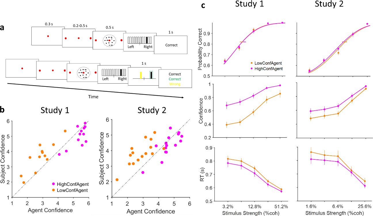
Experiment paradigm and behavioral results.
(a) Timeline of trials in isolated (top) and social (bottom) conditions. After stimulus presentation, subjects reported their decision and confidence simultaneously by clicking on 1 of the 12 vertical bars. In the social condition, decision and confidence of participant (white in the experiment, here black for illustration purpose) and partner (yellow) were color coded. (b) Confidence matching. Participants confidence against agent confidence show a significant relation in both studies (linear regression p<0.001 for both studies). (c) Under social condition, when participants were paired with high (magenta) vs low (dark orange) confidence partner, accuracy (top panel) did not change (horizontal lines, 68% confidence interval of bootstrap test with 10,000 repetitions) but confidence (middle panel) and reaction time (RT) (bottom panel) were altered. Curves fitted to the accuracy data are Weibull cumulative distribution function. Error bars are standard error of the mean (SEM) across subjects.
Figure 1—figure supplement 1

Accuracy and confidence of the computer generated partners (CGPs).
Confidence is plotted in blue and accuracy is plotted in red. (a) Study 1 – HAHC: high accuracy and high confidence. HALC: high accuracy and low confidence. LAHC: low accuracy and high confidence. LALC: low accuracy and low confidence. Error bars: standard deviation across trials. Top-right, bottom-left, and bottom-right are same as top-left but for HALC, LAHC, and LALC, respectively. (b) Study 2 – same as (a) but for 2 CGPs and across 15 partners generated for 15 participants. HCA: high confidence agent; LCA: low confidence agent.
Figure 1—figure supplement 2

Statistical analysis of the confidence matching effect.
(a) Top: Permutation test. The empirically observed difference in mean confidence (red line) is significantly different from the distribution of the expected mean (black curve and dotted line) under null hypothesis (), random pairing, (p~0 for both studies). Bottom: Probability density function (green curve) over confidence matching index defined as (). Dots denote Δm for each combination of 12 participants by 4 computer generated partners (CGPs). The mean confidence difference is significantly different from zero (study 1, p<0.001, paired t-test t(47)=5.5, study 2: p=0.11 t(29)=1.59 but significantly different for HCA condition, p<0.001 t(14)=4.02). (b) Same as (a) but for the second study in which we had 2 CGPs.
Figure 1—figure supplement 3

Examination of the hypothesis that the partner’s confidence at trial t modulates the participant behavior at trial t+1.
Probability correct: First row, confidence: Second row and reaction time (RT): last row. Study 1: first column. Study 2: second column. We used a generalized linear mixed model (GLMM) similar to that used in Figure 1c and plotted the model’s coefficient estimating the impact of partner’s confidence in trial t on the dependent variable of interest in trial t+1. The effects of trial-by-trial variation of partner’s confidence on participant’s confidence and RT were significant and qualitatively similar to what was observed in Figure 1. See Table 1.
Figure 1—figure supplement 4

Summary of debriefing results of the second study.
(a) Participants felt that their partner was more confident when facing with a high confidence agent (HCA). This means our manipulation indeed worked. (b) Similar to (a) but for accuracy. Here, subject did not feel any difference between HCA and low confidence agent (LCA) accuracies. Error bars are SEM across participants.
Figure 2 with 2 supplements
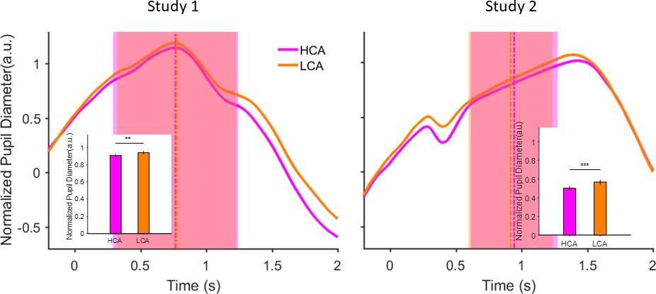
Pupil size during inter-trial interval (ITI) under pairing conditions in the social context when participant was paired with a high (HCA) or low confidence (LCA) agent.
Normalized pupil diameter aligned to start of ITI period (t=0). Vertical dashed lines show average ITI duration. The shaded areas are one standard deviation of ITI period in each condition. Inset shows grand average (mean) pupil size during ITI under the two social conditions. Error bars are 95% confidence interval across trials. (**) indicates p<0.01 and (***) shows p<0.001. In the interest of clarity, signals were smoothed using an averaging filter.
Figure 2—figure supplement 1
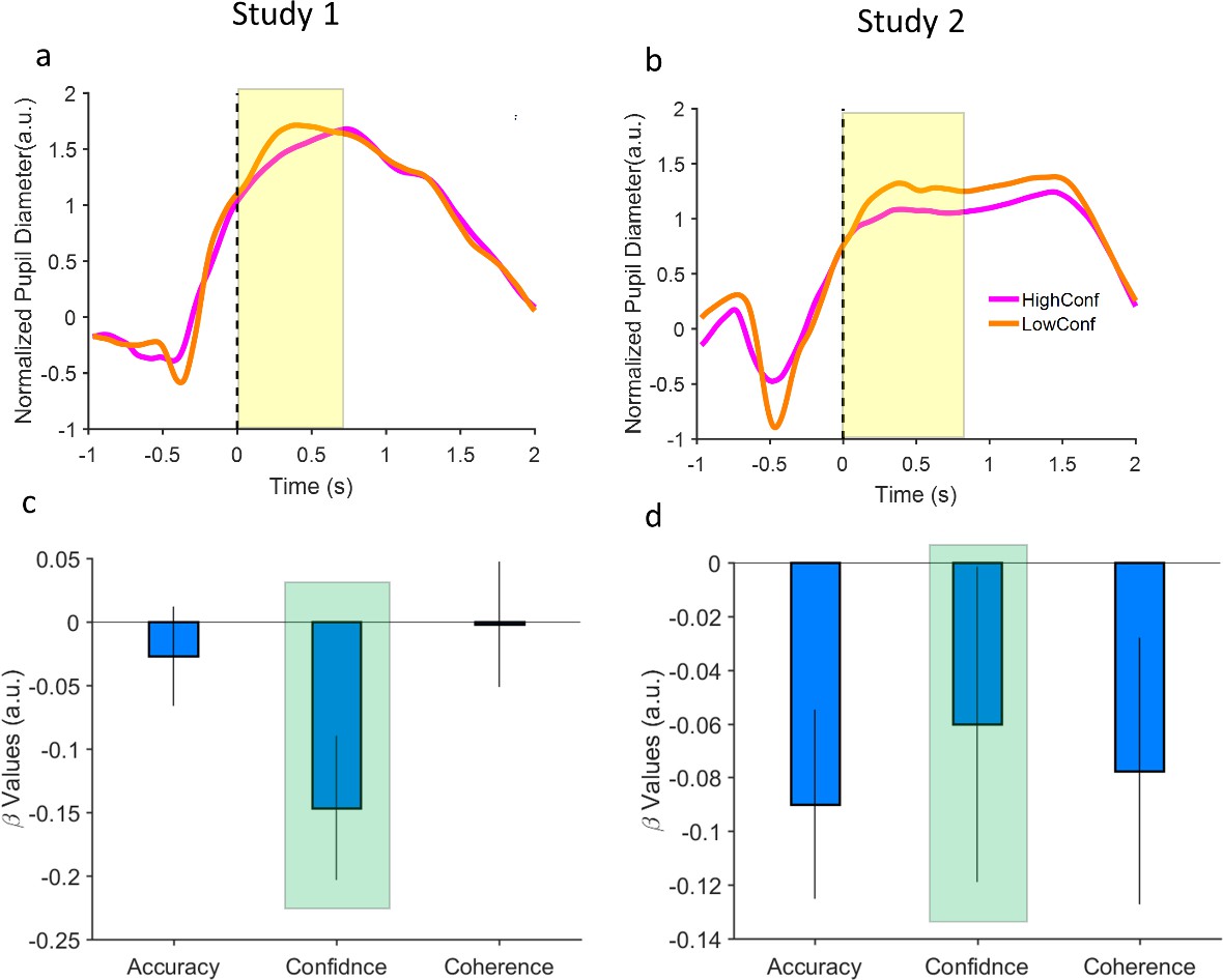
Pupil size correlates with participant’s own confidence in the isolated condition.
(a) In study 1, when confidence was lowest (i.e. rated 1) pupil size was larger (orange curve) than highest confidence (rated 6, magenta curve). The shaded area indicates the average inter-trial interval starting from 0. (b) Study 2. (c) Regression betas from analysis of the impact of confidence on the pupil data in the isolated blocks. The generalized linear mixed model (GLMM) was: PupilData = b0+b1*Accuracy+b2*confidence+b3*Coherence. b2, the highlighted bar, shows the effect of confidence while the effect of coherence and accuracy are regressed out. PupilData is the average pupil size across the ITI period. Error bars are 95% CI. (d) same as (c) but for study (2).
Figure 2—figure supplement 2
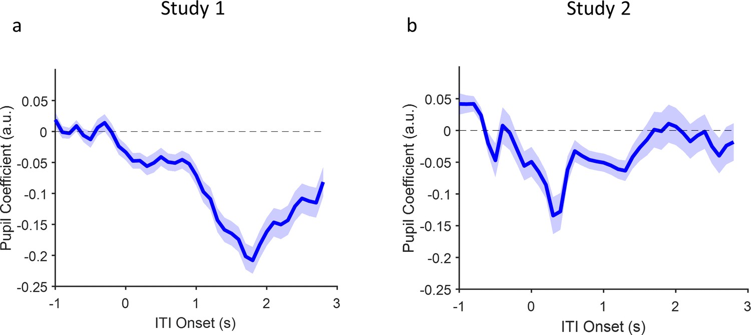
Time series analysis of pupil size during inter-trial interval.
For each study, we employed a generalized linear mixed model (GLMM) Pupil(t)=b0+b1*socialCondition where socialCondition is high confidence agent (HCA) = 1 or low confidence agent (LCA) = 2. The time course of coefficient b1 is plotted with the corresponding SEs. We discretized time into non-overlapping bins of 100 ms width and averaged the data points falling within each bin. (a) Study 1. (b) Study 2.
Figure 3 with 8 supplements
Neural attractor model.
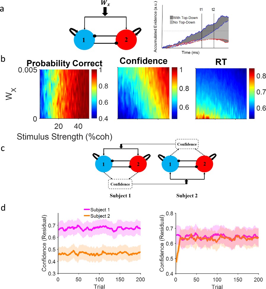
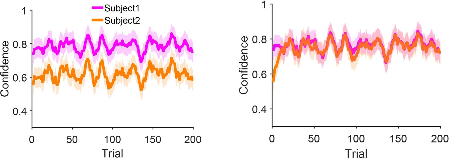
(a) Left: A common top-down (Wx) current drives both populations, each selective for a different choice alternative. Right: A schematic illustration of the impact of a positive top-down drive on accumulator dynamics. Confidence corresponds to the shaded area between winning (blue) and losing (red) accumulators. Solid lines and dark gray shade: positive top-down drive; dashed lines and light gray shade: zero top-down drive. With positive top-down current, the winner hits the bound earlier (t1 vs t2) and the surface area between the competing accumulator traces is larger (dark vs light gray). (b) Systematic examination of the impact of Wx on model behavior. Left panel: Accuracy does not depend on the top-down current but confidence (middle) and reaction time (RT) (right) change accordingly. Colors indicate different levels of top-down current. Each curve is the average of 10,000 simulations of the model given the top-down current. (c) Dynamic coupling in simulated dyadic interaction. Virtual dyads were constructed by feeding one model’s confidence in previous trial to the other model as top-down drive and vice versa. (d) Left: Unconnected virtual dyad members (Wx = 0) simulate the isolated condition. Right: When the virtual dyad members are connected with top-down drive proportional to one another’s confidence in previous trial, dyad members’ confidence converge over time. In the isolated condition, confidence matching is not observed even though the pair receive the exact same sequence of stimuli. Shadowed areas of the confidence interval 95% resulted from 50 parallel simulations and curves were smoothed by an averaging filter for clearer illustration. The correlation with coherence has been removed from the confidence values via residual analysis (see Figure 3—figure supplement 1 confidence values).
Figure 3—figure supplement 1
Confidence matching without removing the correlation with the shared stimulus coherence.
Figure 3—figure supplement 2

The effect of top-down current on the attractor network.
The results of model simulations with a specific value of top-down current (Wx = 0.003). This plot shows the average accumulated evidence of the model in 1000 repetitions with (solid lines) and without (dashed lines) top-down current for a 0.5 s duration of stimulus with 6.4% coherency. Importantly, the network was shut down after stimuli offset, receiving only the noise terms (Equations 7; 8) for 2 s (i.e. more than reaction times [RTs] of 99% of trials). The dot-dashed black line indicates the decision threshold. Inset plots show how the accuracy (ACC), absolute difference of firing rates of two populations (In-Out), and decision time (Dec. Time) changed in the presence (black bars) or absence (white bars) of the top-down current. (***) indicates p<0.001, paired t-test between runs; n.s. denotes that there is no significant difference between conditions.
Figure 3—figure supplement 3
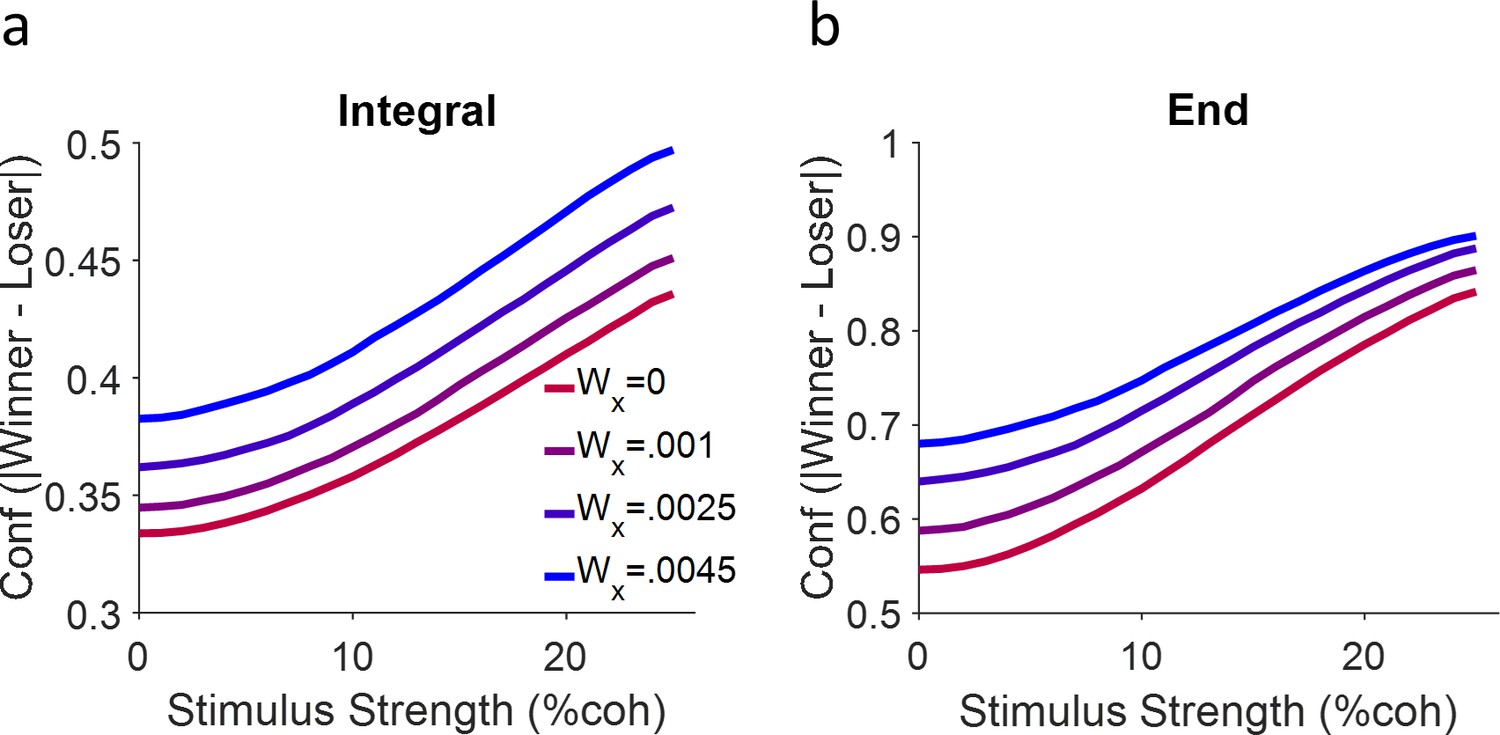
Model performance regarding different confidence representations.
(a) Confidence representation based on Equation 15. (b) Same as (a) but here confidence is calculated as the absolute difference of the winner and loser signal but only at the end of the stimulus duration (500 ms). Each curve is a simulation of 10,000 trials.
Figure 3—figure supplement 4

Model comparison.
We fit each model to the data from high confidence agent (HCA) and low confidence agent (LCA) blocks of each subject (N=15 (subjects) * 2 (blocks)=30). (a) Pie chart indicates the distribution of best (winning) model for the subjects and conditions. (b) Model comparison for each subjects (panels: subject number) in HCA condition (N=15). (c) Same as (b) but for LCA.
Figure 3—figure supplement 5

Model vs data.
(a–c) Correspondence between behavioral data (black circles, 40 trials per coherence level in the isolated session) and the model fits (red curves, simulation with 1000 trials per coherence level) plotted for each participant (n=15). Error bars are SEM across trials. (d) The average behavior across participants was closely captured by the average of model simulations in panel (a–c). Here, error bars are SEM across participants. Shaded area is the SEM across model simulations correspondent to each subject.
Figure 3—figure supplement 6

The speed of confidence matching.
(a) Empirical data depicting the time course of confidence matching. The difference between the subject’s confidence and that of the agent (y-axis) are averaged within a three-trial time window and plotted. To empirically examine the speed of confidence matching we have plotted the empirically observed timeline of confidence matching in the two studies. Here, the absolute difference between the confidence of the agent and that of the subject is plotted against the trial number which indicates time. Observing the curves suggests that confidence matching starts quickly and then slows down as indicated by our simulations. The empirical data is, naturally, noisier but the results do indicate that most of the matching happens at the very beginning. Shaded areas are SEM across participants. Signals were smoothed for illustration purposes. (b–d) Simulations of the modified model where the top-down current was modulated by time. Higher values of the time constant decrease the speed of matching. (b) We applied a different version of top-down current, in which the amount of top-down current is dependent to trial number ( where i is the trial number and is the speed parameter. is the asymptote value: dashed line). Lower values of indicates faster matching (c) rather than higher values of (d) that indicates slower matching.
Figure 3—figure supplement 7
Model falsification.
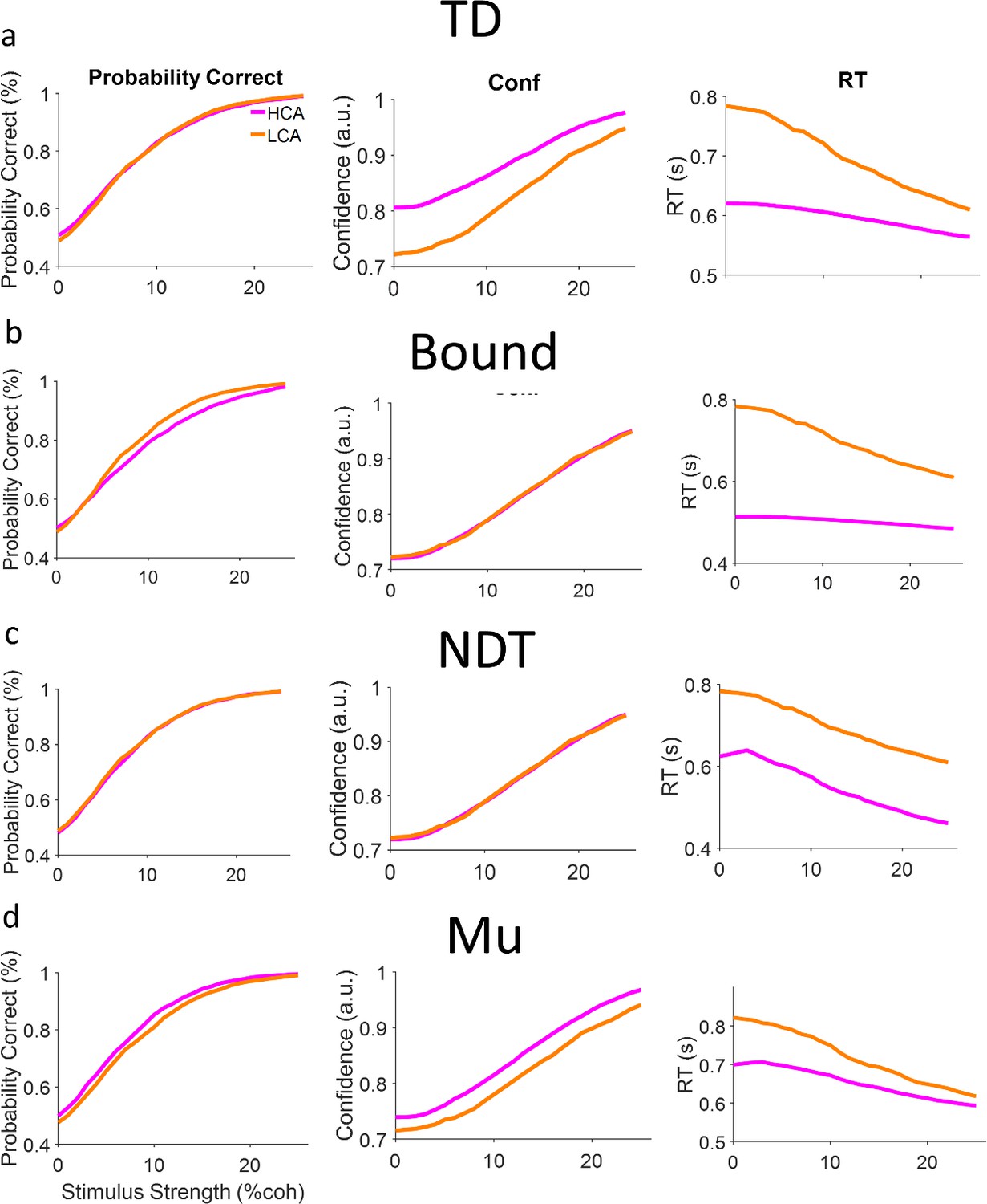
(a) Top-down model. We simulated two versions of the model (2000 trials per coherence level) in which only top-down current was different between conditions (TD in high confidence agent [HCA] is higher than low confidence agent [LCA]). The model could show effects similar to behavior (Figure 1c). (b) Same as (a) but for the bound model. This model could only reproduce the reaction time (RT) effect but not accuracy and confidence effect. (c) Same as (a) but the non-decision time (NDT) model. This model could show the no difference effect in accuracy, yet the confidence also does not change which is not in line with behavioral data (Figure 1c, main text). Moreover, the RT also changes in way that is stimulus independent that is also not similar to the behavioral pattern. (d) Same as (a) but for the Mu (gain) model. The model fails to reproduce accuracy effect. Moreover, the difference of confidence observed in this model is not stimulus/coherence dependent (unlike TD simulations (a) and behavioral data Figure 1c). See also https://github.com/Jimmy-2016/ConfMatchEEG/tree/main/test_alternative_models, ( Esmaily, 2023; MathWorks Inc, 2023) for trying different values of parameters.
Figure 3—figure supplement 8
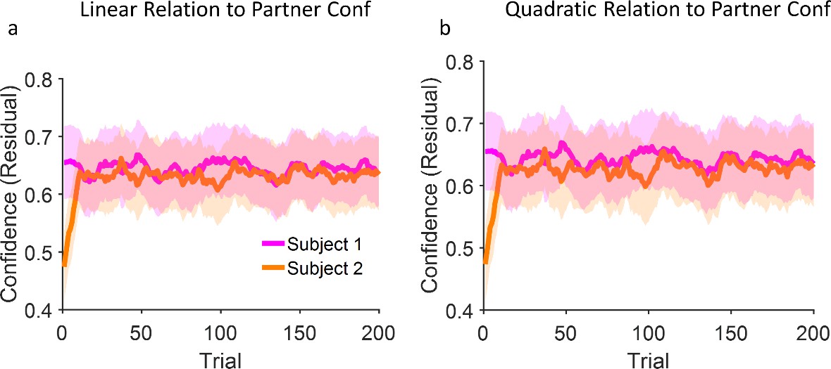
Model predictions for confidence matching are not sensitive to linearity assumptions.
(a) Replication of Figure 3b of the main text in which two models are coupled linearly (see Equation 18) and show confidence matching. (b) Same as (a) but with quadratic coupling. In order to show the robustness of our findings to dropping the linearity assumption, we conducted another analysis in which the two instances of the model interact via a quadratic relationship (Wx = α * Conf2). Here, α was set to –0.001 and 0.006 for high confident and low confident models respectively, while every other parameter as well as the random seed were frozen. The results are very similar to the linear model (panel (a) and also Figure 3d). Indeed, our model is only sensitive to Wx as we shown in Figure 3b. As long as this parameter changes in response to the partner’s confidence, the exact form of the relationship i.e., linear or quadratic, with the partner’s confidence is not important.
Figure 4 with 5 supplements
Coupling of neural evidence accumulation to social exchange of information.
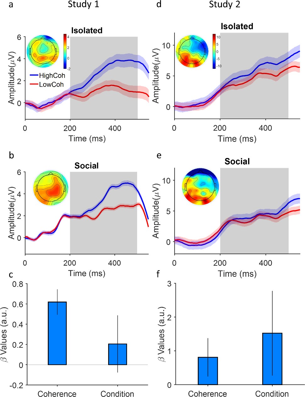
(a) Centroparietal positivity (CPP) component in the isolated condition: event-related potentials are time-locked to stimulus onset, binned for high and low levels of coherency (for study 1, low: 3.2%, 6.4%, 12.8%; high: 25.6% and 51.2%; for study 2 (d), low: 1.6%, 3.2%, 6.4%; high: 12.8%, 25.6%) and grand averaged across centropatrial electrodes (see Materials and methods). Inset shows the topographic distribution of the EEG signal averaged across the time window indicated by the gray area. (b) CPP under social condition. Conventions the same as panel (a). (c) A generalized linear mixed model (GLMM) model showed the significant relation of centroparietal signals to levels of coherency and social condition (high confidence agent [HCA] vs low confidence agent [LCA]). Error bars are 95% confidence interval over the model’s coefficient estimates. Signals were smoothed by an averaging filter; shaded areas are SEM across trials.
Figure 4—figure supplement 1

Electrode placement in each study.
Figure 4—figure supplement 2

Relation of EEG signals from centropartial area of the brain to coherence levels and social conditions.
Top-left, ramping activities of the signals (calculated by a linear regression of signals amplitudes and the time windows of 0–500 ms) is modulated by coherence levels (generalized linear mixed model [GLMM] study 1: p<0.001, study 2 (top-right): p=0.01). Bottom-left: relation of signals slope and social condition (high confidence agent [HCA] vs low confidence agent [LCA]) based on different coherence levels. HCA shows a steeper slope (see Figure 4 and Supplementary file 1c for more details). Right column is the same as left column but for study 2.
Figure 4—figure supplement 3

Simulated slope of the accumulator activity in our computational model in low confidence agent (LCA) and high confidence agent (HCA) conditions.
(a) Slope of the winning accumulator (time window: 0–500 ms; shaded area, insets) at each coherence level for LCA and HCA condition. (b) Same as panel (a) but here for the difference in accumulator activities. Error bars are SEM across trials (n=3000, for each model).
Figure 4—figure supplement 4

Response-locked EEG signal separated for high vs low coherence levels.
(a) As expected from previous studies (Kelly and O’Connell, 2013; Loughnane et al., 2018; O’Connell et al., 2018; Vafaei Shooshtari et al., 2019) centropareital positivity (CPP) signals to high vs low coherence stimulus converge to one another around the moment of response (dashed line, Wilcoxon rank sum test p=0.35). (b) Study 2. It is worth noting that previous studies that examined response-locked CPP employed reaction time (or long duration) tasks with variable stimulus duration. In our study, however, stimulus duration was short and fixed. Our data therefore provide a new addition to this literature confirming response-locked CPP do not depend on termination of stimulus by response.
Figure 4—figure supplement 5

Power calculation (Monte Carlo simulation) for EEG slope effect (Figure 4 in the main manuscript).
Our power calculator suggests we need 17 participants. EEG slope effect was the only effect that was not statistically significant in the first study.
Author response image 1

Calibration plot for the experimental setup.
Average pupil size (arbitrary units from eyelink device) is plotted against display luminance. The plot is obtained by presenting the participant with uniform full screen displays with 10 different luminance levels covering the entire range of the monitor RGB values (0 to 255) whose luminance was separately measured with a photometer. Each display lasted 10 seconds. Error bars are standard deviation between sessions.
Tables
Table 1
Details of statistical results in behavioral data (Figure 1).
| Response | Regressors | Estimate | SE | CI | t-Stat | p-Value | Total number | |
|---|---|---|---|---|---|---|---|---|
| Study 1 | Accuracy (HC vs LC) | Coherency | 0.007 | 0.0006 | [0.006 0.008] | 11.57 | <0.001 | 9600 |
| Condition | –0.002 | 0.021 | [–0.045 0.04] | –0.1 | 0.92 | 9600 | ||
| Confidence (HC vs LC) | Coherency | 0.0475 | 0.0008 | [0.046 0.049] | 56.5 | <0.001 | 9600 | |
| Condition | 1.361 | 0.03 | [1.31 1.42] | 46.4 | <0.001 | 9600 | ||
| RT (HC vs LC) | Coherency | –0.005 | 0.0001 | [–0.005 –0.004] | –44.4 | <0.001 | 9600 | |
| Condition | 0.029 | 0.004 | [–0.035 –0.021] | 7.85 | <0.001 | 9600 | ||
| Study 2 | Accuracy (HC vs LC) | Coherency | 0.0209 | 0.0016 | [0.017 0.024] | 13.23 | <0.001 | 6000 |
| Condition | –0.0092 | 0.0296 | [–0.067 0.049] | –0.31 | 0.76 | 6000 | ||
| Confidence (HC vs LC) | Coherency | 0.1011 | 0.1011 | [0.097 0.106] | 47.47 | <0.001 | 6000 | |
| Condition | 0.496 | 0.037 | [0.42 0.56] | 13.32 | <0.001 | 6000 | ||
| RT (HC vs LC) | Coherency | –0.009 | 0.0003 | [–0.01 –0.008] | –26.22 | <0.001 | 6000 | |
| Condition | 0.0363 | 0.006 | [0.024 0.048] | 6.12 | <0.001 | 6000 |
Table 2
Details of statistical results in pupil data (Figure 2).
| Response | Regressors | Estimate | SE | CI | t-Stat | p-Value | Total number | |
|---|---|---|---|---|---|---|---|---|
| Study 1 | Pupil | Condition | –0.038 | 0.011 | [–0.06 –0.01] | –3.30 | <0.001 | 8390 |
| Study 2 | Pupil | Condition | –0.066 | 0.015 | [–0.09 –0.04] | –4.37 | <0.001 | 5842 |
Table 3
Details of statistical results in EEG data (Figure 4).
| Response | Regressors | Estimate | SE | CI | t-Stat | p-Value | Total number | |
|---|---|---|---|---|---|---|---|---|
| Study 1 | EEG slope | Coherency | 0.62 | 0.065 | [0.49. 074] | 9.64 | <0.001 | 6492 |
| Condition | 0.2 | 0.14 | [-0.07 0.49] | 1.42 | 0.15 | 6492 | ||
| Study 2 | EEG slope | Coherency | 0.8 | 0.29 | [0.24 1.37] | 2.8 | <0.01 | 5367 |
| Condition | 1.52 | 0.63 | [0.27 2.77] | 2.39 | 0.017 | 5367 |
Table 4
Details of statistical results in EEG data (Figure 4—figure supplement 2 top row).
| Response | Regressors | Estimate | SE | CI | t-Stat | p-Value | Total number | |
|---|---|---|---|---|---|---|---|---|
| Study 1 | EEG slope | Coherency | 0.02 | 0.005 | [0.01 0.03] | 4.48 | <0.001 | 1523 |
| Study 2 | EEG slope | Coherency | 0.06 | 0.02 | [0.01 0.11] | 2.54 | <0.01 | 2822 |
Table 5
Details of statistical results for the impact of previous trial (Figure 1—figure supplement 3).
| Response | Regressors | Estimate | SE | CI | t-Stat | p-Value | Total number | |
|---|---|---|---|---|---|---|---|---|
| Study 1 | Accuracy (HC vs LC) | Coherency | 0.007 | 0.0006 | [0.006 0.008] | 11.58 | <0.001 | 9600 |
| Conf (t–1) | –0.0017 | 0.005 | [–0.01 0.01] | –0.28 | 0.77 | 9600 | ||
| Confidence (HC vs LC) | Coherency | 0.047 | 0.001 | [0.045, 0.049] | 54.7 | <0.001 | 9600 | |
| Conf (t–1) | 0.32 | 0.008 | [0.3 0.33] | 38.31 | <0.001 | 9600 | ||
| RT (HC vs LC) | Coherency | –0.005 | 0.0001 | [–0.0048 0.0044] | –44.36 | <0.001 | 9600 | |
| Conf (t–1) | –0.0055 | 0.001 | [–0.007 –0.003] | –5.44 | <0.001 | 9600 | ||
| Study 2 | Accuracy (HC vs LC) | Coherency | 0.02 | 0.002 | [0.02 0.024] | 13.23 | <0.001 | 6000 |
| Conf (t–1) | 0.003 | 0.008 | [–0.012 0.018] | 0.37 | 0.7 | 6000 | ||
| Confidence (HC vs LC) | Coherency | 0.1 | 0.002 | [0.097 0.0106] | 47.2 | <0.001 | 6000 | |
| Conf (t–1) | 0.09 | 0.01 | [0.07 0.11] | 8.6 | <0.001 | 6000 | ||
| RT (HC vs LC) | Coherency | –0.009 | 0.0003 | [–0.001 –0.008] | –26.2 | <0.001 | 6000 | |
| Condition | 0.005 | 0.001 | [0.001 0.008] | 2.98 | <0.01 | 6000 |
Table 6
The rate of trial rejection of eye tracking (only data of social) and EEG data (visual inspection) per participant.
| Participants | Eye tracking rejection % (social) | EEG trial rejection % (visual) | |
|---|---|---|---|
| Study 1 (Discovery) | 1 | 12.25 | 4.6 |
| 2 | 12.87 | 31.1 | |
| 3 | 0.5 | 22.1 | |
| 4 | 4 | 14.8 | |
| 5 | 1.37 | 34.4 | |
| 6 | 0 | 4.6 | |
| 7 | 7.75 | 8.8 | |
| 8 | 0.37 | 24.4 | |
| 9 | 6.37 | 7.6 | |
| 10 | 0 | 46 | |
| 11 | 0.12 | NA | |
| 12 | NA | NA | |
| Study 2 (Replication) | 1 | 0 | 4 |
| 2 | 1.25 | 1 | |
| 3 | 5.75 | 8.5 | |
| 4 | 0.5 | 3 | |
| 5 | 1 | 16 | |
| 6 | 1.5 | 2.5 | |
| 7 | 0 | 0.5 | |
| 8 | 1.5 | 9 | |
| 9 | 0 | 2 | |
| 10 | 1 | 4 | |
| 11 | 1 | 7.5 | |
| 12 | 0.5 | 0 | |
| 13 | 0.75 | 10.5 | |
| 14 | 2.5 | 12 | |
| 15 | 14.75 | 4.5 |
Table 7
Generalized linear mixed model (GLMM) including interaction terms (p-values are reported).
| Response | Coherence | Condition (LC vs HC) | Condition* coherence | |
|---|---|---|---|---|
| Study 1 | Accuracy | p<0.001 | p=0.92 | p=0.96 |
| Confidence | p<0.001 | p<0.001 | p<0.001 | |
| RT | p<0.001 | p<0.001 | p<0.05 | |
| Pupil | p=0.43 | p=0.20 | p=0.31 | |
| EEG slope | p<0.01 | p=0.15 | p=0.91 | |
| Study 2 | Accuracy | p<0.001 | p=0.75 | p=0.87 |
| Confidence | p<0.001 | p<0.001 | p<0.001 | |
| RT | p<0.001 | p<0.001 | p=0.34 | |
| Pupil | p=0.35 | p=0.06 | p=0.17 | |
| EEG slope | p=0.62 | p<0.05 | p=0.68 |
Table 8
Attractor model’s parameters.
| Parameter | Parameter value | Reference, remarks |
|---|---|---|
| JN,ii | 0.3157 nA | Calibrated based on pool of isolated data, also fitted on individual subjects’ data |
| JN,ij | 0.0646 nA | Calibrated based on pool of isolated data, also fitted on individual subjects’ data |
| µ0 | 45.8 Hz | Calibrated based on pool of isolated data, also fitted on individual subjects’ data |
| NDT | 0.27 s | Calibrated based on pool of isolated data, also fitted on individual subjects’ data |
| Bound | 0.32 nA | Calibrated based on pool of isolated data, also fitted on individual subjects’ data |
| a (Equation 15) | –0.99 | Calibrated based on pool of isolated data, also fitted on individual subjects’ data |
| b0 (Equation 15) | 1.32 | Calibrated based on pool of isolated data, also fitted on individual subjects’ data |
| b1 (Equation 15) | –0.165 | Calibrated based on pool of isolated data, also fitted on individual subjects’ data |
| k (Equation 15) | 5.9 | Calibrated based on pool of isolated data, also fitted on individual subjects’ data |
| I0 | 0.3255 nA | From Wang, 2002; Wong and Wang, 2006 |
| JA.ext | 0.00022 nA Hz–1 | From Wang, 2002; Wong and Wang, 2006 |
| τs | 0.1 s | From Wang, 2002; Wong and Wang, 2006 |
| dt | 0.0005 s | From Wang, 2002; Wong and Wang, 2006 |
| a (Equation 13) | 270 (V nC)–1 | From Wang, 2002; Wong and Wang, 2006 |
| b (Equation 13) | 108 Hz | From Wang, 2002; Wong and Wang, 2006 |
| d (Equation 13) | 0.154 s | From Wang, 2002; Wong and Wang, 2006 |
| γ | 0.641 | From Wang, 2002; Wong and Wang, 2006 |
| Noise_std | 0.025 | From Wang, 2002; Wong and Wang, 2006 |
| I_noise | 0.02 | From Wang, 2002; Wong and Wang, 2006 |
Additional files
-
MDAR checklist
- https://cdn.elifesciences.org/articles/83722/elife-83722-mdarchecklist1-v1.pdf
-
Supplementary file 1
This file contains supplementary tables that contains details of statistical analysis.
- https://cdn.elifesciences.org/articles/83722/elife-83722-supp1-v1.docx
Download links
A two-part list of links to download the article, or parts of the article, in various formats.
Downloads (link to download the article as PDF)
Open citations (links to open the citations from this article in various online reference manager services)
Cite this article (links to download the citations from this article in formats compatible with various reference manager tools)
Interpersonal alignment of neural evidence accumulation to social exchange of confidence
eLife 12:e83722.
https://doi.org/10.7554/eLife.83722


