Generative network modeling reveals quantitative definitions of bilateral symmetry exhibited by a whole insect brain connectome
- Department of Biomedical Engineering, Johns Hopkins University, United States
- Department of Biostatistics, Johns Hopkins University, United States
- Department of Zoology, University of Cambridge, United Kingdom
- Neurobiology Division, MRC Laboratory of Molecular Biology, United Kingdom
- Janelia Research Campus, Howard Hughes Medical Institute, United States
- Department of Applied Mathematics and Statistics, Johns Hopkins University, United States
Figures
Figure 1
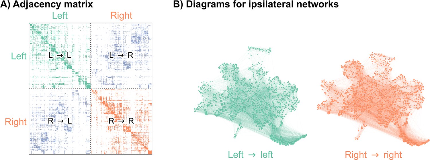
Visualizations of a larval Drosophila brain connectome from Winding et al., 2023.
(A) Adjacency matrix for the full brain connectome network, sorted by brain hemisphere. Note that we ignore the left → right and right → left (contralateral) subgraphs in this work. (B) Network layouts for the left → left and right → right subgraphs.
-
Figure 1—source data 1
Drosophila larva brain connectome.
- https://cdn.elifesciences.org/articles/83739/elife-83739-fig1-data1-v2.zip
Figure 2
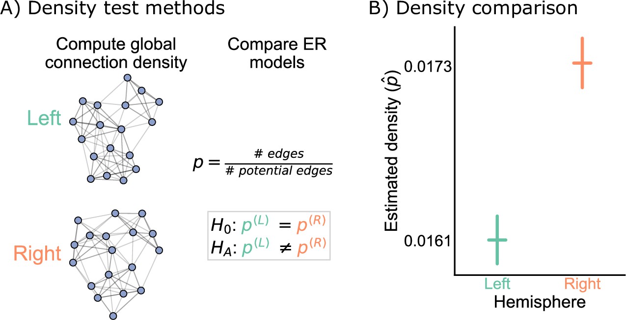
Comparison of left and right hemisphere networks via the density test.
(A) Diagram of the methods used for testing based on the network density. See Erdos-Renyi model and density testing for more details. (B) The estimated density (probability of any edge averaged across the entire network) for the left hemisphere is ~0.016, while for the right it is ~0.017 – this makes the left density ~0.93 that of the right. Vertical lines denote 95% confidence intervals for this estimated parameter . The p-value for testing the null hypothesis that these densities are the same is (two-sided chi-squared test), meaning very strong evidence to reject the null that the left and right hemispheres have the same density.
Figure 3 with 5 supplements
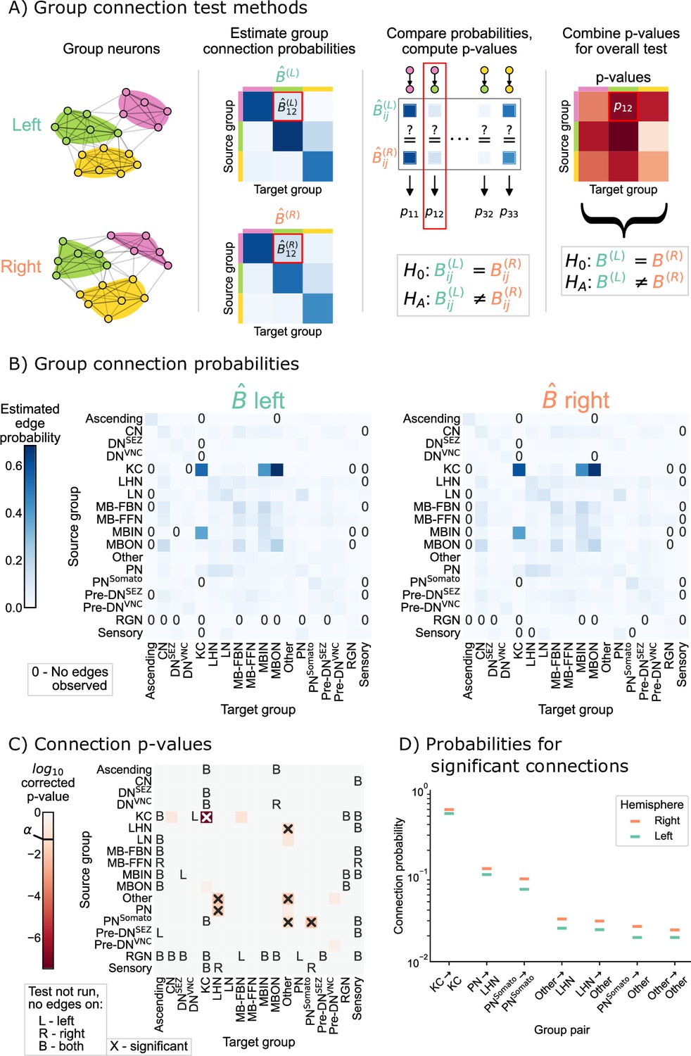
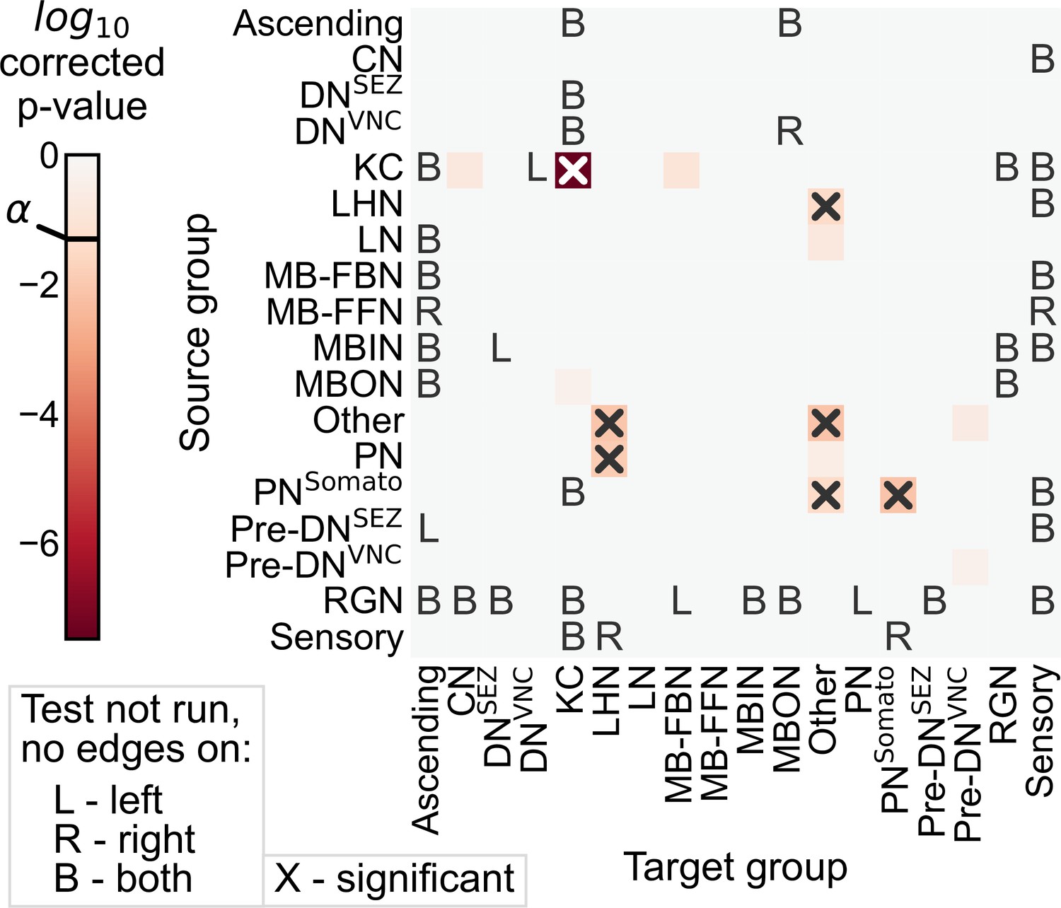
Comparison of left and right hemisphere networks via the group connection test.
(A) Description of methodology for the group connection test. See SBMs and group connection testing for more details. (B) Estimated group-to-group connection probabilities for both hemispheres. Note that they appear qualitatively similar. Estimated probabilities which are zero (no edge was present between that pair of groups) are indicated with a ‘0’ in those cells. (C) p-Values (after multiple comparisons correction) for each hypothesis test between individual elements of the connection probability matrices. Each cell represents a test for whether a specific group-to-group connection probability is the same on the left and right sides. ‘X’ denotes a significant p-value after multiple comparisons correction, with significance level . ‘B’ indicates that a test was not run since the estimated probability was zero on both hemispheres, ‘L’ indicates this was the case on the left only, and ‘R’ that it was the case on the right only. The individual (uncorrected) p-values were combined using Tippett’s method, resulting in an overall p-value (for the null hypothesis that the two group connection probability matrices are the same) of . (D) Comparison of estimated group-to-group connection probabilities for the group pairs that are significantly different. In each case, the connection probability on the right hemisphere is higher.
Figure 3—figure supplement 1
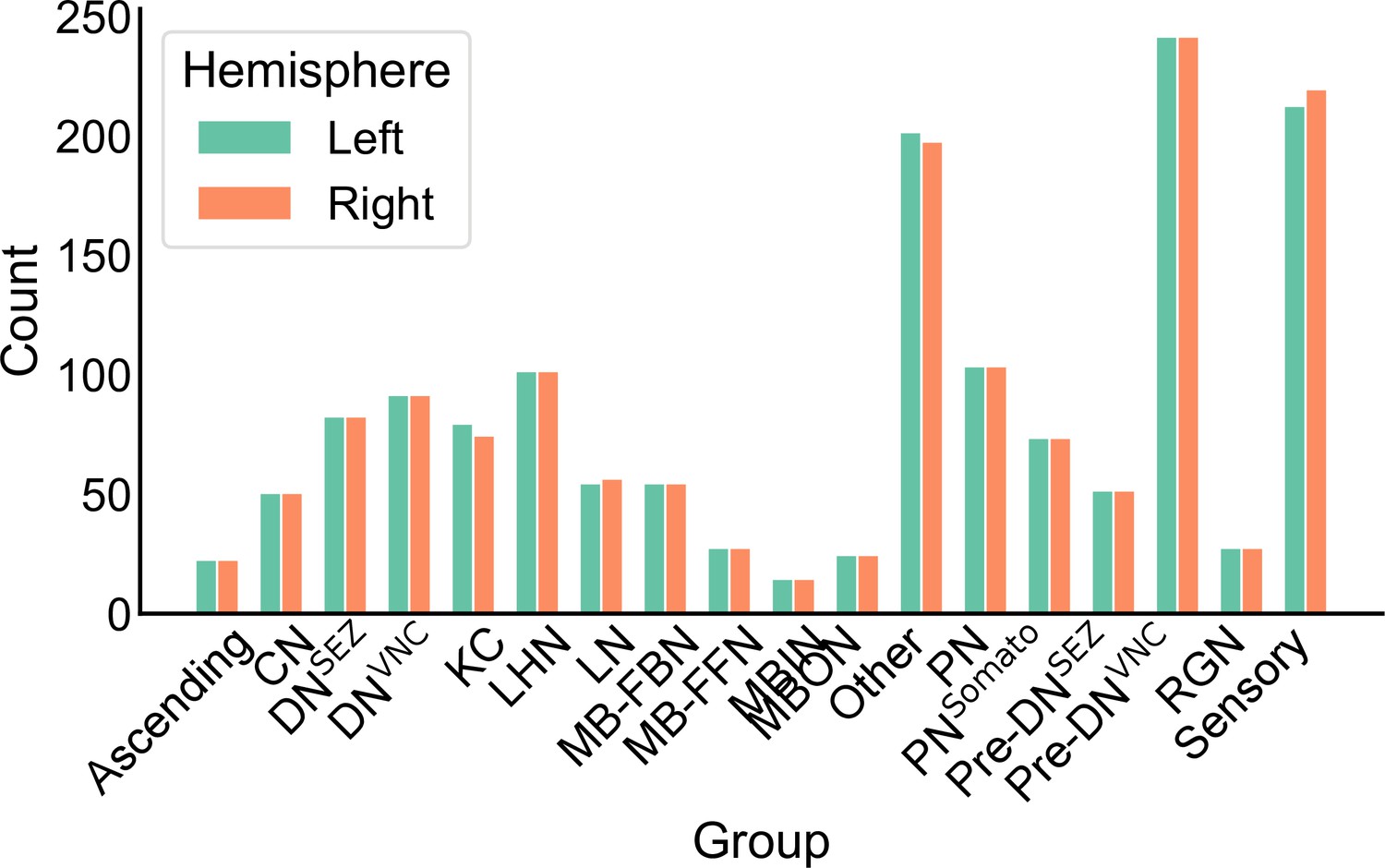
The number of neurons in each neuron group in the left and right hemispheres.
Figure 3—figure supplement 2
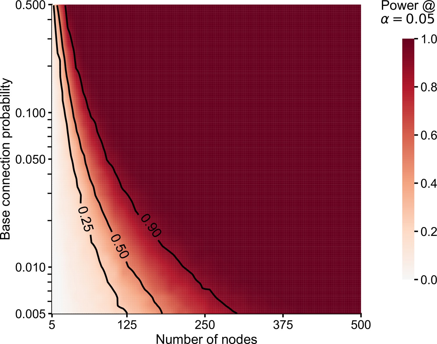
Empirical power (in simulations) for tests comparing subgraph connection probabilities (chi-squared test, i.e. each component test in the group connection test).
Simulated data (edge counts) were sampled from a for one subgraph, and for the other. represents the number of nodes in each subgraph and (base connection probability) represents the probability of an edge in this subgraph (subgraph density). For a varying number of nodes () and base connection probability (), we sampled 1000 times from the two binomial models above, and then ran chi-squared tests (two-sided) on each pair of sampled data. The heatmap displays empirical power (probability of correctly rejecting the null hypothesis of equal connection probabilities) as a function of the number of nodes and base connection probability, with lines showing level sets for a power of 0.25, 0.5, and 0.9. Note that power increases both as the number of nodes (and thus, the number of possible edges) increases, but also as the connection probability approaches 0.5.
Figure 3—figure supplement 3
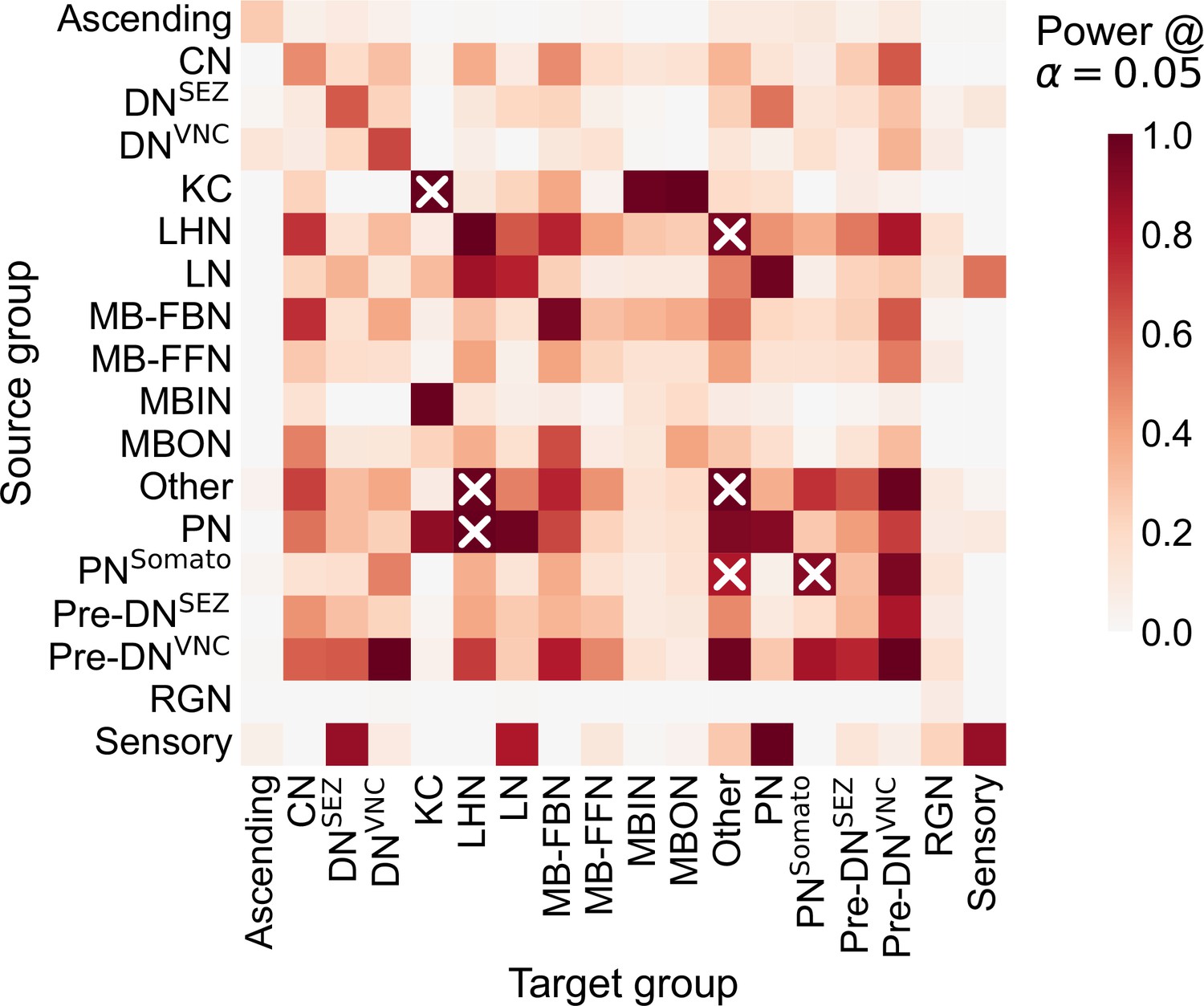
Estimated empirical power for each component of the group connection test in simulations based on the observed Drosophila larva brain connectome.
Simulation setting was similar to that in Figure 3—figure supplement 2, comparing data (edge counts) sampled from vs. via a two-sided chi-squared test. Here, n1 and n2 were the number of nodes for each of the two groups being compared, respectively, in the Drosophila larva brain connectome from Winding et al., 2023. was set to the mean connection probability for that subgraph across the left and right hemispheres. Heatmap displays empirical power across 1000 samples for this simulation setting, plotted as a function of the subgraphs being compared. ‘X’ denotes subgraphs which were significantly different in Group connection test.
Figure 3—figure supplement 4
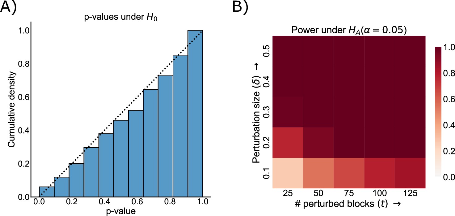
Demonstration that the group connection test is both valid and powerful against a range of alternatives in a synthetic simulation based on the observed data.
See Power and validity of group connection test under various alternatives for more details on the simulation. (A) Cumulative distribution of p-values from Tippett’s method for combining p-values under the null, where the two group connection matrices and are the same. Note that the distribution of these p-values is sub- , i.e., below the dashed line indicating the cumulative distribution of a random variable, meaning that the test is valid and the Type-I error is properly controlled for any level . (B) Power (probability of correctly rejecting the null hypothesis when it is false) as a function of the number of perturbed blocks () and the strength of each perturbation (). The test is powerful against both a small number of strong perturbations and a large number of small perturbations, indicating its general applicability.
Figure 3—figure supplement 5
p-Values from the group connection test (as described in Figure 3), but using Fisher’s exact test for each individual subgraph comparison.
The p-value for the overall test is . Note that the same subgraphs are found to be significant as in Figure 3.
Figure 4 with 1 supplement
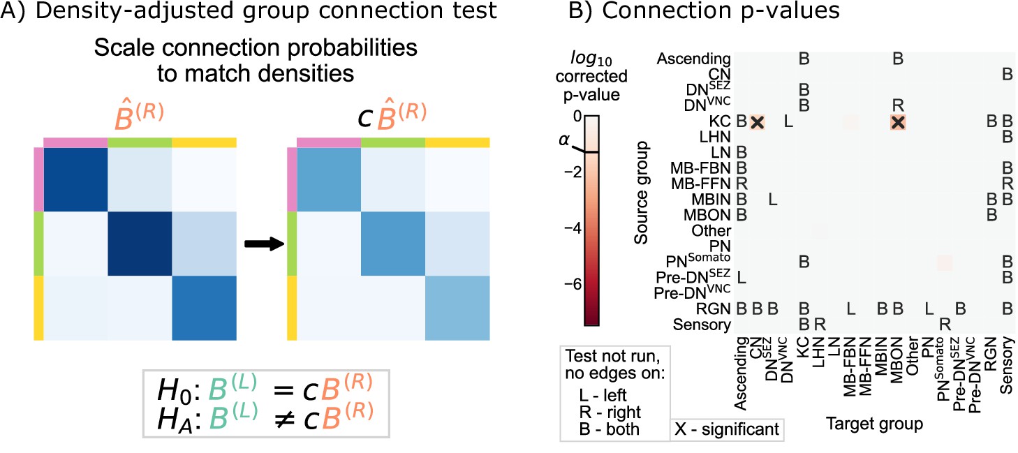
Comparison of left and right hemisphere networks via the density-adjusted group connection test.
(A) Description of methodology for adjusting for a density difference between the two stochastic block models. See SBMs and group connection testing for more details. The adjustment factor (ratio of the left to the right density), c, is ~0.93. (B) p-Values for each group-to-group comparison after adjusting for a global density difference. p-Values are shown after correcting for multiple comparisons. Note that there are two significant p-values, and both are in group connections incident to Kenyon cells. These individual (uncorrected) p-values were combined using Tippett’s method, resulting in an overall p-value (for the null hypothesis that the two group connection probability matrices are the same after correcting for the density difference) of .
Figure 4—figure supplement 1
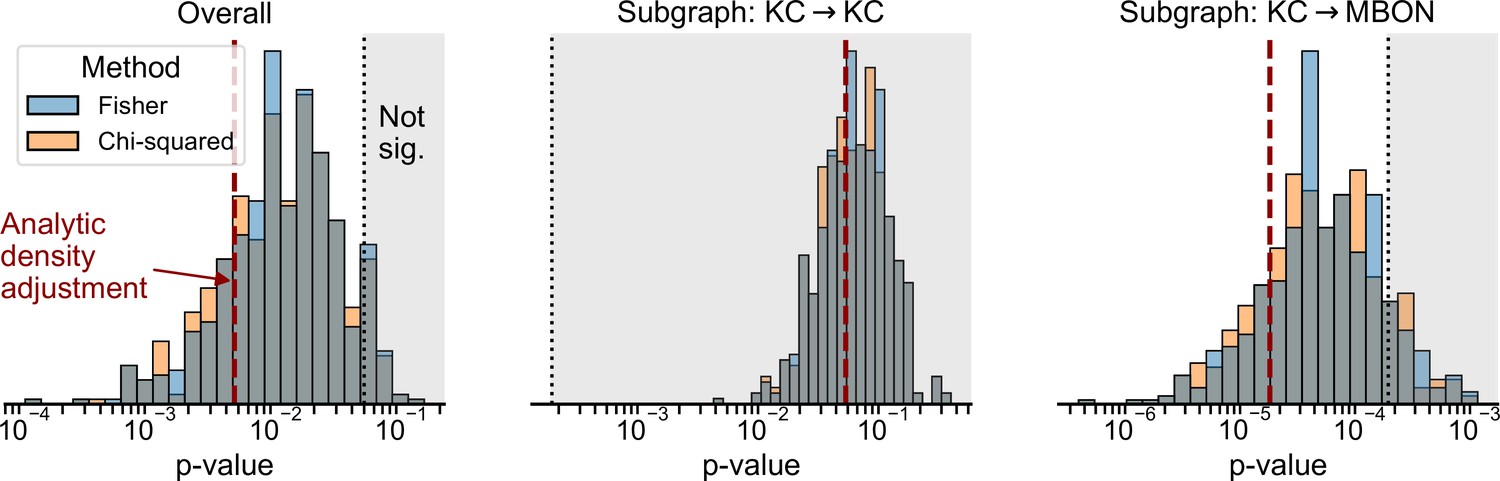
Distribution of p-values from experiments in which 2760 edges were randomly removed from the right hemisphere to set the densities of the left and right hemispheres equal, and the group connection test was re-run.
p-Values are shown for the overall test (left), as well as the individual p-values for the KC → KC (center) and KC → MBON (right) as example subgraphs. Distributions show p-values from 500 random edge removal experiments for both Fisher’s exact test and the chi-squared test. Dashed red line shows the single p-value from the analytic density-adjusted test used in Figure 4. Dashed black line and shaded regions indicate the p-values which were not significant at significance level 0.05 (left), or at the corresponding Bonferroni-adjusted level for the subgraph tests (center and right).
Figure 5
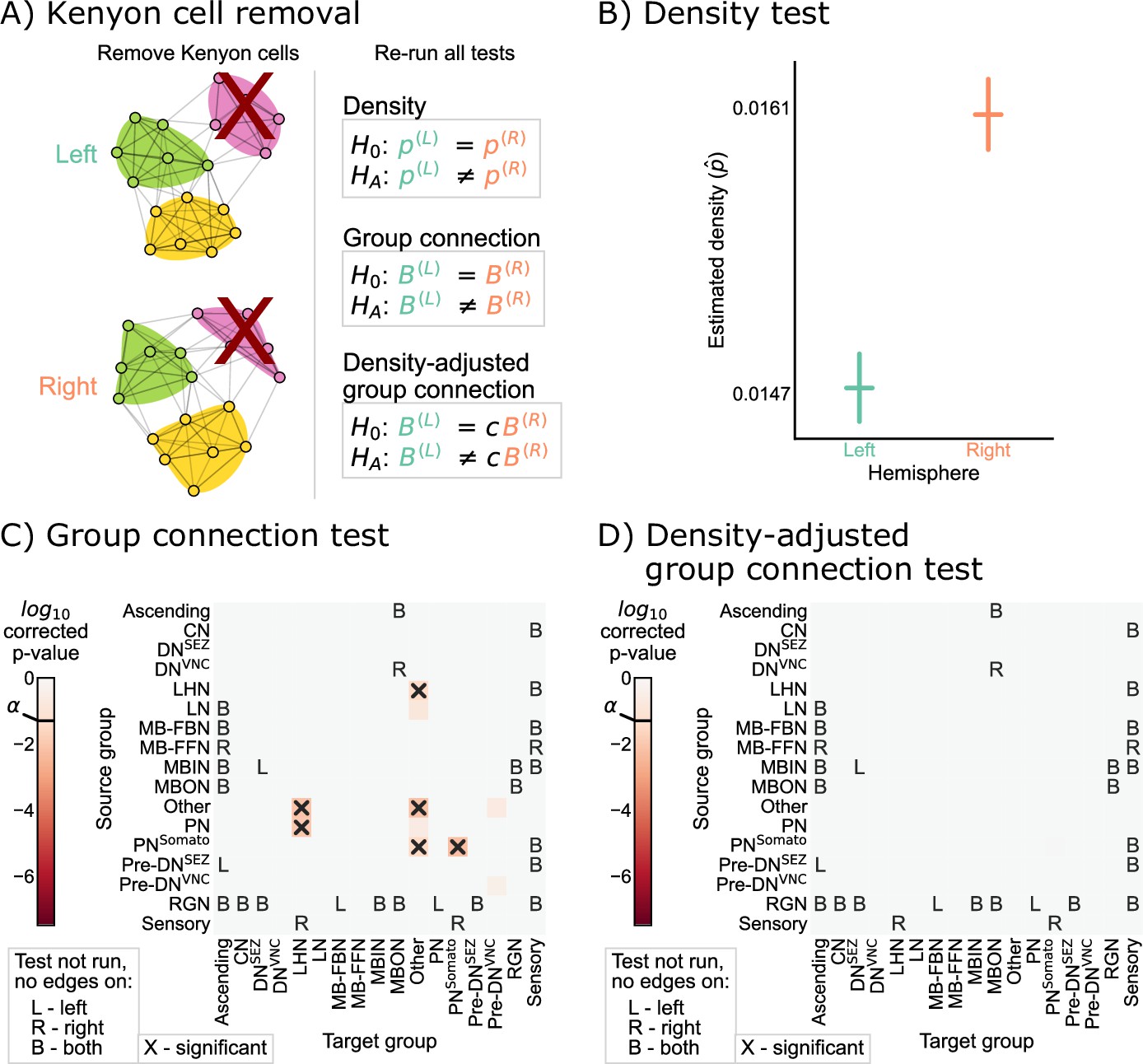
Comparison of left and right hemisphere networks when not including Kenyon cells.
(A) Diagram of the methods used, indicating that Kenyon cells (and any incident edges) were simply removed from the network, and all previously mentioned tests were run again. (B) Comparison of network densities, as in Figure 2B. The p-value for this comparison is , indicating very strong evidence to reject the null that the two networks share the same density. (C) Comparison of group-to-group connection probabilities, as in Figure 3C. p-Values are shown for each group-to-group connection comparison (after multiple comparison correction). The (uncorrected) p-values were combined to yield an overall p-value of , showing evidence that the group connection probabilities are not the same even after removing Kenyon cells. (D) Comparison of group-to-group connection probabilities after density adjustment, as in Figure 4C. p-Values are shown for each group-to-group connection comparison (after multiple comparison correction). Note that there are no longer any significantly different connections. The (uncorrected) p-values were combined to yield an overall p-value of ~0.60. After removing Kenyon cells, there is no longer evidence to reject the null that the group connection probabilities are the same.
Figure 6 with 1 supplement
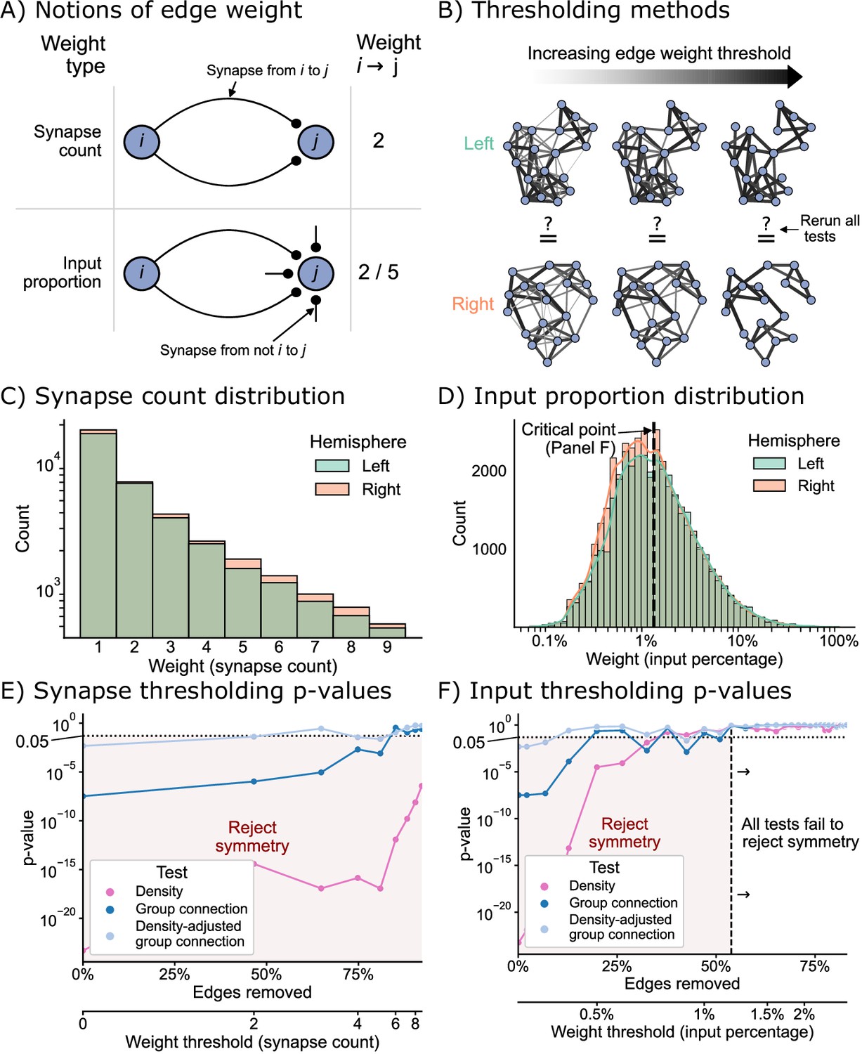
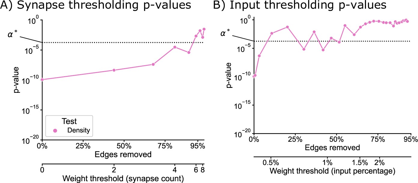
The effect of edge weight threshold on the significance level for each of the tests of bilateral symmetry.
Diagrams of (A) two notions of edge weight and (B) application of edge weight thresholds to examine bilateral symmetry. See Edge weight thresholds for more explanation. (C) Distribution of synapse count edge weights. The right hemisphere consistently has more edges in each synapse count bin. (D) Distribution of input percentage edge weights. The right hemisphere has more edges in the lower () portion of this distribution, but the hemispheres match well for high edge weights. (E) p-Values for each test after synapse count thresholding, plotted as a function of the percentage of edges which are removed from the networks, as well as the corresponding weight threshold (lower x-axis). The p-values for all tests generally increased as a function of synapse count threshold, but the density test never reached a p-value >0.05 over this range of thresholds. (F) p-Values for each test after input percentage thresholding, plotted as a function of the percentage of edges which were removed from the networks, as well as the corresponding weight threshold (lower x-axis). Note that all tests yielded insignificant (>0.05) p-values after a threshold of around 1.25% input proportion. Compared to the results in (E), thresholding based on input percentage reached insignificant p-values faster as a function of the total amount of edges removed for all tests.
Figure 6—figure supplement 1
p-Values for left/right comparisons as a function of edge weight thresholds (as in Edge weight thresholds), but performed only on the KC → KC subgraph.
Dashed line () indicates a Bonferonni-corrected significance level of 0.05, using the total number of tests run in Group connection test. The qualitative trends observed for the entire network hold for this subgraph in isolation, where for both thresholding methods p-values generally increase as the threshold increases, and this effect happens faster for the input percentage thresholding.
Author response image 1
Author response image 2
Tables
Table 1
Neuron group definitions, categorizations from Winding et al., 2023.
| Acronym | Full name |
|---|---|
| Ascending | Ascending neurons from the ventral nerve cord |
| CN | Convergence neurons, receiving input from lateral horn and mushroom body |
| DNSEZ | Descending neurons (to the sub-esophageal zone) |
| DNVNC | Descending neurons (to the ventral nerve cord) |
| KC | Kenyon cells |
| LHN | Lateral horn neurons |
| LN | Local neurons |
| MB-FBN | Mushroom body feedback neurons |
| MB-FFN | Mushroom body feedforward neurons |
| MBIN | Mushroom body input neurons |
| MBON | Mushroom body output neurons |
| Other | Neurons lacking any other categorization |
| PN | Projection neurons |
| PNSomato | Somatosensory projection neurons |
| Pre-DNSEZ | Neurons projecting to DNSEZs |
| Pre-DNVNC | Neurons projecting to DNVNCs |
| RGN | Ring gland neurons |
| Sensory | Sensory neurons |
Table 2
Summary of tests, models, hypotheses, whether Kenyon cells (KC) were included, and the resulting p-values for each evaluation of bilateral symmetry.
| Test method | Model | (vs ) | KC | p-Value |
|---|---|---|---|---|
| Density test | ER | + | ||
| Group connection test | SBM | + | ||
| Density-adjusted group connection test | DA-SBM | + | ||
| Density test | ER | - | ||
| Group connection test | SBM | - | ||
| Density-adjusted group connection test | DA-SBM | - | ~0.60 |
Additional files
Download links
A two-part list of links to download the article, or parts of the article, in various formats.
Downloads (link to download the article as PDF)
Open citations (links to open the citations from this article in various online reference manager services)
Cite this article (links to download the citations from this article in formats compatible with various reference manager tools)
Generative network modeling reveals quantitative definitions of bilateral symmetry exhibited by a whole insect brain connectome
eLife 12:e83739.
https://doi.org/10.7554/eLife.83739


