The functional form of value normalization in human reinforcement learning
- Laboratoire de Neurosciences Cognitives et Computationnelles, Institut National de la Santé et Recherche Médicale, France
- Département d’Etudes Cognitives, Ecole Normale Supérieure, PSL University, France
- Department of Psychology, University of Hamburg, Germany
Figures
Figure 1
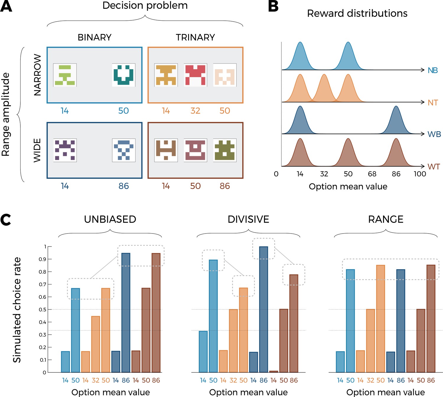
Experimental design and model predictions of Experiment 1.
(A) Choice contexts in the learning phase. Participants were presented with four choice contexts varying in the amplitude of the outcomes’ range (narrow or wide) and the number of options (binary or trinary decisions). (B) Means of each reward distribution. After each decision, the outcome of each option was displayed on the screen. Each outcome was drawn from a normal distribution with variance . NB: narrow binary, NT: narrow trinary, WB: wide binary, WT: wide trinary. (C) Model predictions of the transfer phase choice rates for the UNBIASED (left), DIVISIVE (middle), and RANGE (right) models. Note that choice rate in the transfer phase is calculated across all possible binary combinations involving a given option. While score is proportional to the agent’s preference for a given option, it does not sum to one because any given choice counts for the final score of two options. Dashed lines represent the key prediction for each model.
Figure 2 with 2 supplements
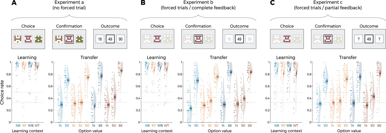
Behavioral results of Experiment 1.
Top: successive screens of a typical trial for the three versions of the main experiment: without forced trials (A), with forced trials and complete feedback information (B) and with forced trials and partial feedback information (C). Bottom: correct choice rate in the learning phase as a function of the choice context (left panels), and choice rate per option in the transfer phase (right panels) for the three versions of the main experiment: without forced trials (A), with forced trials and complete feedback information (B) and with forced trials and partial feedback information (C). In all panels, points indicate individual average, shaded areas indicate probability density function, 95% confidence interval, and SEM (n=50). NB: narrow binary, NT: narrow trinary, WB: wide binary, WT: wide trinary.
Figure 2—figure supplement 1
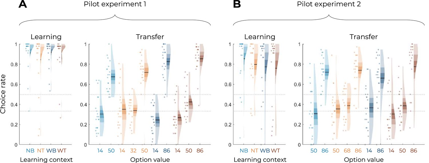
Behavioral results of the pilot Experiment similar to Experiments 1 and 2.
Correct choice rate in the learning phase as a function of the choice context (left panels), and choice rate per option in the transfer phase (right panels) for pilot Experiment 1 (A) and pilot Experiment 2 (B). In all panels, points indicate individual average, shaded areas indicate probability density function, 95% confidence interval, and SEM. NB: narrow binary, NT: narrow trinary, WB: wide binary, WT: wide trinary. To ascertain that our task design would be feasible and that participants would be able to learn the values of 10 options by trial-and-error, a pilot online-based experiment was originally performed. We recruited 40 participants (23 females, 16 males, 1 N/A, aged 30.35 ± 9.73 y) via Prolific (https://www.prolific.co). In the pilot experiments, the outcome variance was set to , that is, the rewards were displayed without any noise (in the main tasks, the variance was set to ). In order to characterize learning behavior of participants, we analyzed the correct response rate in the learning and the transfer phases, that is, choices directed toward the most favorable option at each trial. To assess successful learning, we first tested participants’ correct response rate against chance level. We found it to be above chance level in both the learning phase (0.5 and 0.33 in the binary and trinary learning contexts, respectively; pilot experiment 1: t(19) = 11.83, p<0.0001, d = 2.65; pilot experiment 2: t(19) = 7.39, p<0.0001, d = 1.65) and the transfer phase (0.5; pilot experiment 1: t(19) = 5.87, p<0.0001, d = 1.31; pilot experiment 2: t(19) = 3.01, p=0.0072, d = 0.67).
Figure 2—figure supplement 2
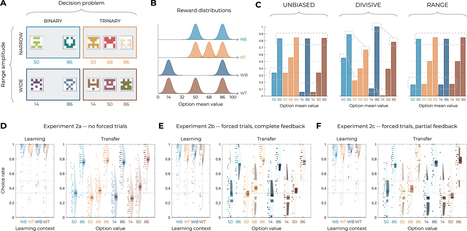
Experimental design, model predictions, and behavioral results concerning Experiment 2.
(A) Choice contexts in the learning phase. Participants were presented with four choice contexts varying in the amplitude of the outcomes’ range (narrow or wide) and the number of options (binary or trinary decisions). (B) Means of each reward distribution. After each decision, the outcome of each option was displayed on the screen. Each outcome was drawn from a normal distribution with variance . NB: narrow binary, NT: narrow trinary, WB: wide binary, WT: wide trinary. (C) Model predictions of the transfer phase choice rates for the UNBIASED (left), DIVISIVE (middle), and RANGE (right) models. Dashed lines represent the key prediction for each model. (D–F) Correct choice rate in the learning phase as a function of the choice context (left panels), and choice rate per option in the transfer phase (right panels) for the three versions of the main experiment: without forced trials (D), with forced trials and complete feedback information (E) and with forced trials and partial feedback information (F). In all panels, points indicate individual average, shaded areas indicate probability density function, 95% confidence interval, and SEM. NB: narrow binary, NT: narrow trinary, WB: wide binary, WT: wide trinary. In addition to Experiment 1, whose results are presented in the main text, we recruited 150 participants to perform a modified version of Experiment 1. The only difference between Experiment 1 and Experiment 2 is the value of the options in the narrow contexts: in Experiment 1, they went from 14 to 50; in Experiment 2, they went from 50 to 86. Similar to Experiment 1, participants were given a bonus depending on the number of points won in the experiment (average money won in pounds: 6.38 ± 0.58, average performance against chance during the learning phase and transfer phase: M = 0.78 ± 0.099, t(149) = 34.65, p<0.0001, d = 2.83). No data had to be excluded for technical issues. In the learning phase, the correct response rate was significantly higher than chance level (0.5 and 0.33 in the binary and trinary learning contexts, respectively) in all conditions (least significant: t(49) = 13.71, p<0.0001, d = 1.94; on average: t(49) = 15.75, p<0.0001, d = 2.23). We further checked whether the task factors affected performance in the learning phase and found a small significant effect of the decision problem (the correct choice rate being higher in the binary compared to the trinary contexts: F(1,49) = 4.11, p=0.048, η2 = 0.08), but no effect of range amplitude (wide versus narrow; F(1,49) = 0.027, p=0.87, η2 = 0.00) or interaction (F(1,49) = 0.92, p=0.34, η2 = 0.02). In the transfer phase, the correct choice rate in the transfer was significantly higher than chance (t(49) = 9.56, p<0.0001, d = 1.35), thus providing positive evidence of value retrieval and generalization (Bavard et al., 2018; Bavard et al., 2021; Hayes and Wedell, 2022). Contrary to what was predicted by the UNBIASED or the DIVISIVE models, the choice rate for the lowest value options (NB50, NT50, WB14, and WT14) did not follow the patterns depicted in panel (C). In fact, all lowest value options displayed a similar choice rate (F(3,49) = 1.85, p=0.14, η2 = 0.04), which is only consistent with the predictions of the RANGE model. Concerning other features of the transfer phase performance, the mid-value options valuation is also consistent with the RANGE model, which predict that these options will be valued equally (NT68 and WT50; t(49) = –1.34, p=0.19, d = −0.19), contrary to the UNIBIASED and DIVISIVE models that both predict NT68 to be greater than WT50. Similar to Experiment 1, these mid-value options displayed a choice rate very close to that of the corresponding lowest value options (NT50 and WT14): this feature is still not perfectly captured by the RANGE model (which predicts their choice rate perfectly in between those of high- and low-value options). To rule out that this effect was not due to a lack of attention for the low- and mid-value options, we also designed two additional experiments where we added forced-choice trials to focus the participants’ attention on all possible options (Table 1). As in Experiment 1, focusing participants’ attention to all possible outcomes by forcing their choice did not significantly affect the behavioral performance neither in the learning phase (F(2,147) = 0.78, p=0.46, η2 = 0.01, Levene’s test F(2,147) = 0.38, p=0.69) nor in the transfer phase (F(2,147) = 0.81, p=0.45, η2 = 0.01, Levene’s test F(2,147) = 0.81, p=0.45). Given the absence of detectable differences across experiments, in the model-based analyses that follow, we pooled the three experiments together. To sum up, the behavioral results are consistent with those of Experiment 1, are in contrast with the predictions of both the UNBIASED and the DIVISIVE models, and are rather consistent with the range normalization process proposed by the RANGE model.
Figure 3 with 3 supplements
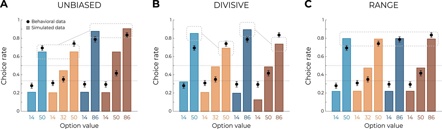
Qualitative model comparison.
Behavioral data (black dots, n=150) superimposed on simulated data (colored bars) for the UNBIASED (A), DIVISIVE (B), and RANGE (C) models. Simulated data in the transfer phase were obtained with the best-fitting parameters, optimized on all four contexts of the learning phase. Dashed lines represent the key prediction for each model.
Figure 3—figure supplement 1
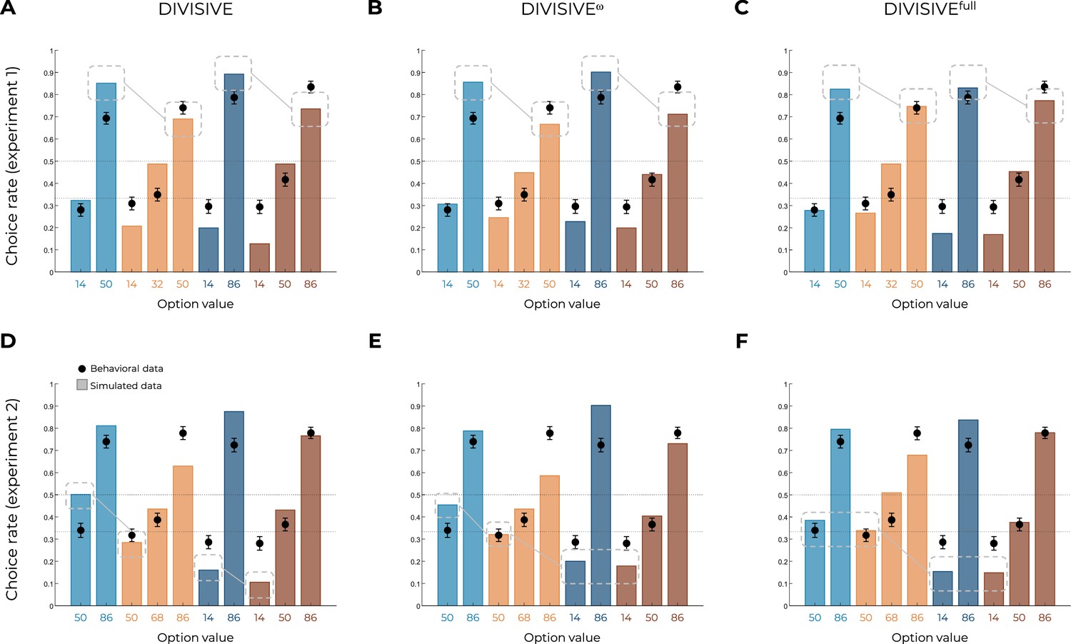
Ruling out more complex forms of divisive normalization.
Behavioral data (black dots, n=150) superimposed on simulated data (colored bars) for Experiment 1 (top row) and Experiment 2 (bottom row), for the DIVISIVE (A, D), DIVISIVEω (B, E), and DIVISIVEfull (C, F) models. Simulated data in the transfer phase were obtained with the best-fitting parameters, optimized on all four contexts of the learning phase. Dashed lines represent the key features that allow discriminating divisive normalization models from range normalization and unbiased value representations. To confirm that our power manipulation in the RANGEω model would not affect our predictions in the DIVISIVE model (especially, the difference in value between options from binary and trinary contexts, e.g., WB86 and WT86), we implemented the same manipulation in the DIVISIVE model. In the DIVISIVEω model, the normalized outcome is power-transformed by the parameter (), as follows: where is the number of contextually relevant stimuli. Crucially, for , the DIVISIVEω model reduces to the DIVISIVE model. As expected, the DIVISIVEω model was unable to match participants’ behavior despite a small improvement in the prediction of the choice rates for mid and lowest value options, in both experiments. Moreover, over both experiments, quantitative model comparison favored the DIVISIVEω model over the DIVISIVE model (oosLLDIV(ω) = −129.25 ± 64.94, median = −116.98; oosLLDIV(ω) vs. oosLLDIV: t(299) = 11.50, p<0.0001, d = 0.66) but not over range-adaptation model (oosLLDIV(ω) vs. oosLLRAN(ω): t(299) = −11.71, p<0.0001, d = −0.68). In conclusion, the addition of a power transformation was insufficient to correct the behavioral predictions of the DIVISIVE model. Finally, we acknowledge that the normalization rule we implemented is a simpler implementation of classical divisive normalization (Louie et al., 2013; Louie et al., 2015; Webb et al., 2021). To make sure that this over-simplification did not affect the main results of this study, we implemented a more complex version of divisive normalization, including a semi-saturation parameter, a normalization weight parameter, and a -norm parameter (Webb et al., 2021): where is the number of contextually relevant stimuli; the parameter determines, in a neural system, how neural activity saturates with increased input and can be interpreted as the baseline activity level in the normalization; the parameter determines the contribution to the normalization from other alternatives; each alternative is scaled by the magnitude and number of its elements by a norm of degree . Crucially, the DIVISIVEfull model is nested within the DIVISIVE and UNBIASED model: when , and , the DIVISIVEfull model reduces to the DIVISIVE model; when and , the DIVISIVEfull model reduces to the UNBIASED model (no normalization). Quantitative model comparison showed a substantial improvement in the ability of the DIVISIVEfull model to fit participants’ data over the simple DIVISIVE model (oosLLDIV(full) = −136.19 ± 88.33, median = −120.63; oosLLDIV(full) vs. oosLLDIV: t(299) = 4.69, p<0.0001, d = 0.27), but not over range adaptation models (oosLLDIV(full) vs. oosLLRAN(ω): t(299) = −10.36, p<0.0001, d = −0.60). These comparisons were consistent with model simulations, which clearly show that the key features of the model fail to predict transfer performance. In conclusion, and unsurprisingly given the structure of the model, the more complex version of the divisive normalization rule was unable to match participants’ behavior in our task.
Figure 3—figure supplement 2
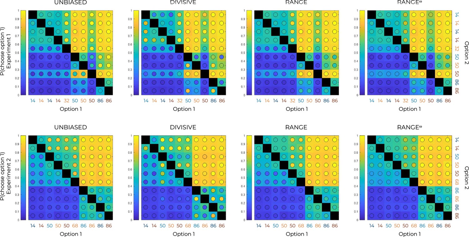
Choice rates per option in the transfer phase and model simulations.
Colored maps of pairwise choice rates during the transfer phase of Experiment 1 (top row) and experiment 2 (bottom row), for each option when compared to each of the nine other options, noted here generically as Option 1 and Option 2 in increasing order. Model simulations (colored circles) are superimposed over behavioral data (colored squares). Comparisons between the same symbols are undefined (black squares).
Figure 3—figure supplement 3
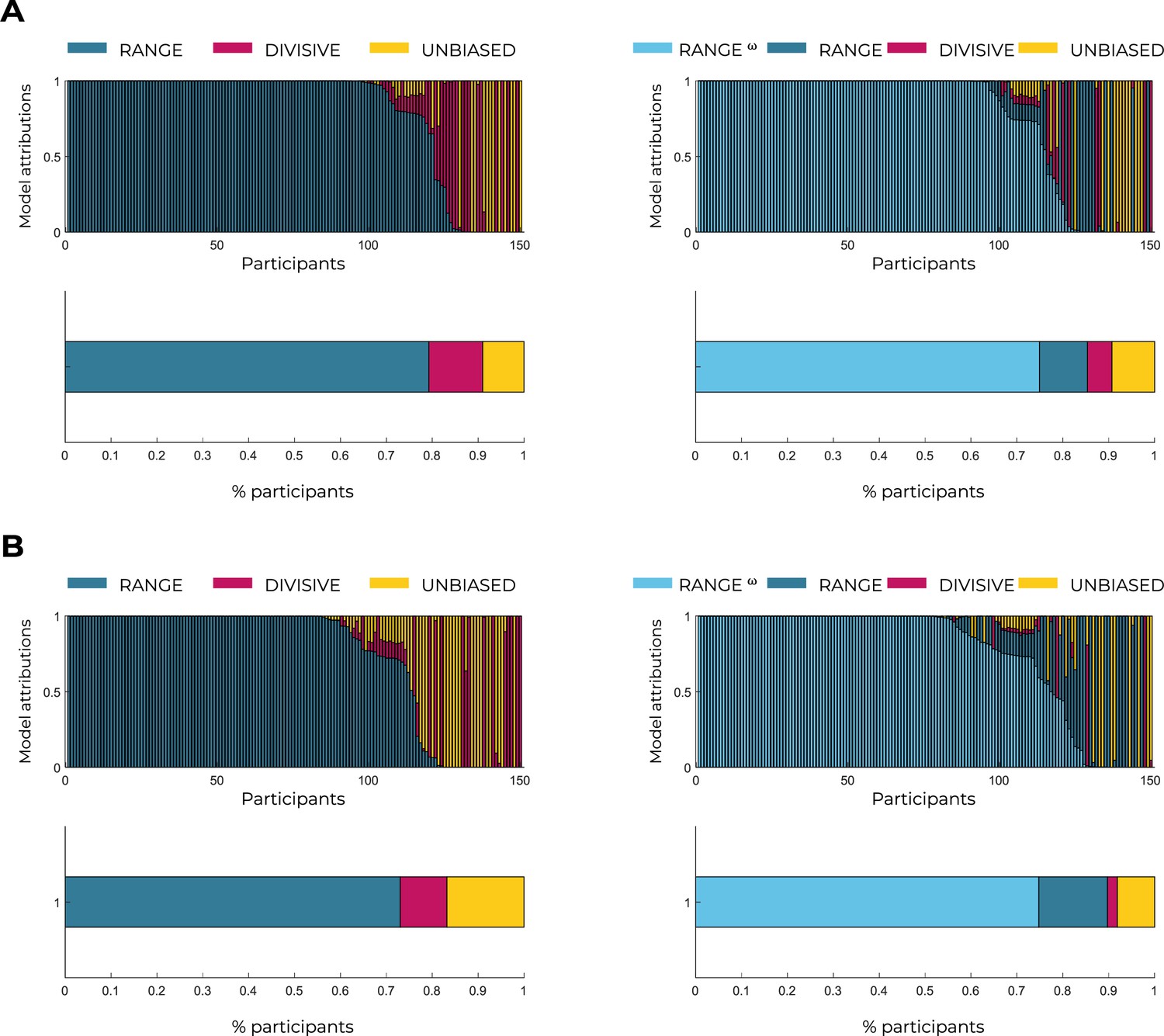
Model attributions across participants.
Model attributions per participant and percentage of participants (n=150) explained by the RANGE, DIVISIVE, UNBIASED (left), and RANGEω (right) models in Experiment 1 (A) and Experiment 2 (B).
Figure 4
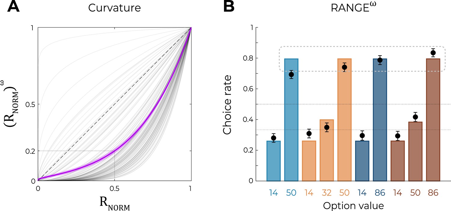
Predictions of the nonlinear RANGE model.
(A) Curvature function of the normalized reward per participant. Each gray line was simulated with the best-fitting power parameter for each participant. Dashed line represents the identity function (), purple line represents the average curvature over participant, and shaded area represents SEM. (B) Behavioral data (black dots, n=150) superimposed on simulated data (colored bars) for the RANGEω model. Simulated data in the transfer phase were obtained with the best-fitting parameters, optimized on all four contexts of the learning phase. Dashed lines represent the key prediction for the model.
Figure 5 with 1 supplement
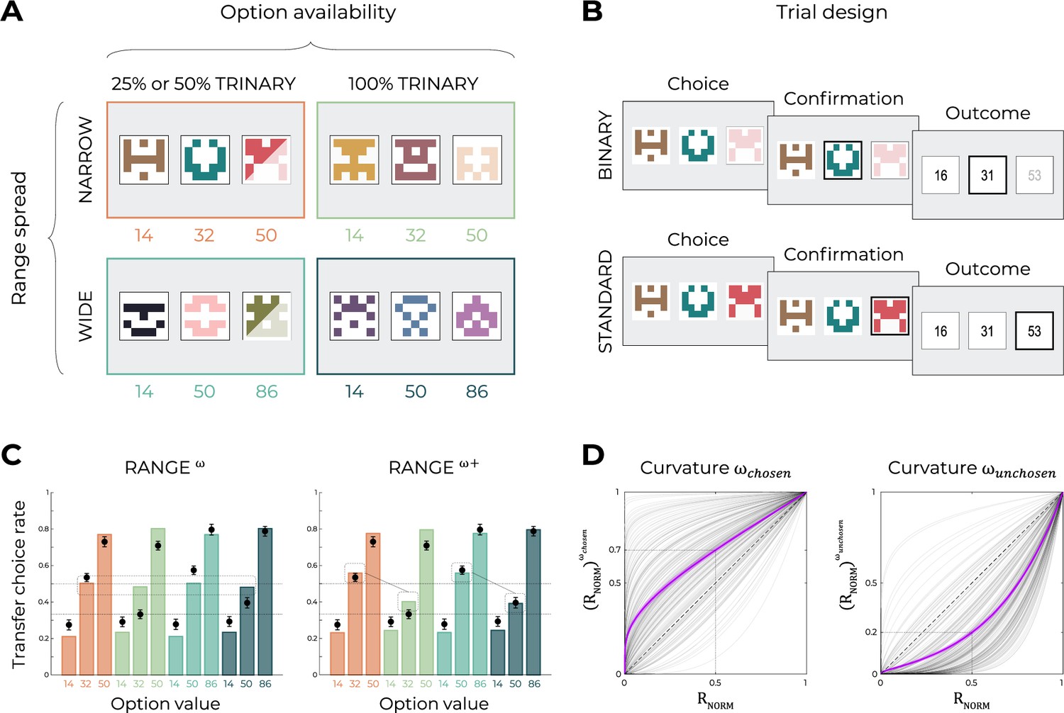
Experimental design and main results of Experiment 3.
(A) Choice contexts in the learning phase. Participants were presented with four choice contexts varying in the amplitude of the outcomes’ range (narrow or wide) and the number of available options (trinary or binary decisions). (B) Trial sequence for a binary trial (50 or 75% of the total number of learning trials), where the high-value option was presented but not available to the participant, and a standard trinary trial (50 or 25% of the total number of learning trials). (C) Behavioral data (black dots, n=200) superimposed on simulated data (colored bars) for the RANGEω and RANGEω+ models. Simulated data in the transfer phase were obtained with the best-fitting parameters, optimized on all four contexts of the learning phase. Dashed lines represent the key prediction for the model. (D) Curvature functions of the normalized reward per participant. Each gray line was simulated with the best-fitting power parameters and for each participant. Dashed line represents the identity function (), purple line represents the average curvature over participant, and shaded area represents SEM. Results in (C) and (D) are pooled data for Experiments 3a and 3b.
Figure 5—figure supplement 1
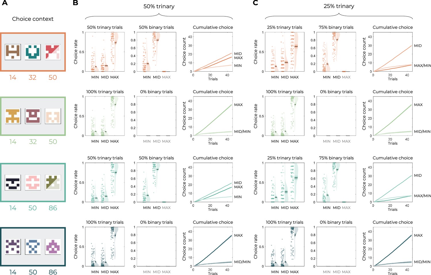
Design and behavioral results of Experiment 3.
(A) Experiment design of Experiments 3a (n=100) and 3b (n=100). All contexts included three options, but one option was not selectable on either 50 or 75% of the learning trials. (B–, C) Behavior results of Experiment 3a (B) and Experiment 3b (C) in each learning context. Left: choice rate in the trinary trials.
Figure 6 with 1 supplement
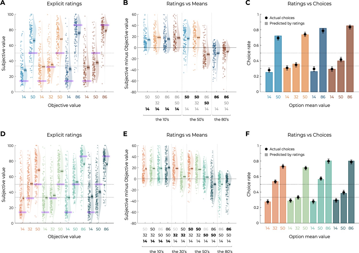
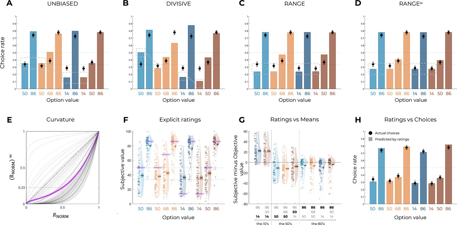
Results from the explicit elicitation phase of Experiments 1 and 3.
(A, D) Reported subjective values in the elicitation phase for each option, in Experiment 1 (A, n=150) and Experiment 3 (D, n=200). Points indicate individual average, and shaded areas indicate probability density function, 95% confidence interval, and SEM. Purple areas indicate the actual objective value for each option. (B, E) Difference between reported subjective value and actual objective value for each option, arranged in ascending order, in Experiment 1 (B) and Experiment 3. The legend of the x-axis represents the values of the options of the context in which each option was learned (actual option value shown in bold). Points indicate individual average, and shaded areas indicate probability density function, 95% confidence interval, and SEM. (C, F) Behavioral choice-based data (black dots) superimposed on simulated choice-based data (colored bars), in Experiment 1 (C) and Experiment 3 (F). Simulated data were obtained with an argmax rule assuming that participants were making transfer phase decision based on the explicit subjective ratings of each option.
Figure 6—figure supplement 1
Qualitative model comparison and explicit ratings of Experiment 2.
Behavioral data (black dots, n=150) superimposed on simulated data (colored bars) for the UNBIASED (A), DIVISIVE (B), RANGE (C), and RANGEω (D) models. Simulated data in the transfer phase were obtained with the best-fitting parameters, optimized on all four contexts of the learning phase. Dashed lines represent the key prediction for each model. (E) Curvature function of the normalized reward per participant. Each gray line was simulated with the best-fitting power parameter for each participant. Dashed line represents the identity function (), purple line represents the average curvature over participant, and shaded area represents SEM. (F) Reported subjective values in the elicitation phase for each option. Points indicate individual average, and shaded areas indicate probability density function, 95% confidence interval, and SEM. Purple areas indicate the actual objective value for each option. (G) Difference between reported subjective value and actual objective value for each option, arrange in ascending order. The legend of the x-axis represents the values of the options of the context in which each option was learned (actual option value shown in bold). Points indicate individual average, and shaded areas indicate probability density function, 95% confidence interval, and SEM. (H) Behavioral choice-based data (black dots) superimposed on simulated choice-based data (colored bars). Simulated data were obtained with an argmax rule assuming that subjects were making transfer phase decisions based on the explicit subjective ratings of each option. Similar to Experiment 1, model comparison favored the RANGE model over to both the DIVISIVE and the UNBIASED models (oosLLRAN vs. oosLLDIV: t(149) = 10.61, p<0.0001, d = 0.87; oosLLRAN vs. oosLLUNB: t(149) = 5.71, p<0.0001, d = 0.47; Table 2). Model simulations also confirmed what inferred from the ex ante simulations and indicated that the RANGE model predicts results much closer to the observed ones in respect of many key comparisons. Model comparison and model simulations of the RANGEω model supported the conclusions from Experiment 1. On average, the power parameter was >1 (mean ± SD: 2.83 ± 1.47, t(149) = 15.25, p<0.0001, d = 1.25), suggesting that participants value the mid-value options less than the midpoint between the lowest and highest options (i.e., closer to the lowest option). Quantitative model comparison favored the RANGEω model over all other models, including the RANGE model (Table 2) (oosLLRAN vs. oosLLRAN(ω): t(149) = −8.63, p<0.0001, d = −0.70; Table 2). Moreover, the inspection of model simulations confirmed that the RANGEω model perfectly captures participants’ behavior in the transfer phase. More specifically, the mid-value options (NT68 and WT50) and the lowest value options (NB14, NT14, WB14, and WT14) were better estimated in all contexts. To conclude, the addition of a power parameter allowed our model to match participants’ behavior almost perfectly. Consistently with the results of Experiment 1, the subjective values elicited through explicit ratings were consistent with those elicited through binary choices in many key aspects. Again, to compare elicitation methods, we simulated transfer phase choices based on the explicit elicitation ratings. We found the pattern simulated using explicit ratings to perfectly match the actual choice rates of the transfer phase (t(149) = 1.18, p=0.24, d = 0.10), suggesting that both elicitation methods tap into the same valuation system.
Author response image 1
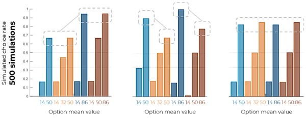
Model predictions generated from 500 simulations.
Author response image 2
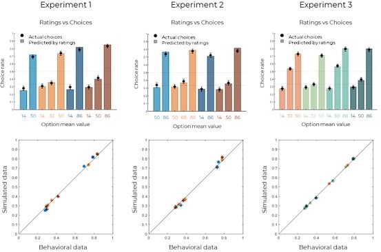
Simulated and behavioral data for the Explicit phase.
Top: behavioral choice-based data (black dots) superimposed on simulated choice-based data (colored bars). Simulated data were obtained using the explicit ratings as values and a argmax decision rule (see Methods). Bottom: average simulated data per option (horizontal error bars) as a function of average behavioral data per option (vertical error bars). Error bars represent s.e.m., plain diagonal line represents idendity.
Author response image 3
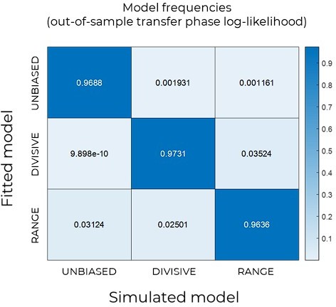
Confusion matrix for model recovery.
For each model, we performed ex-ante simulations following the procedure described in the Methods section. We then fitted the simulated data with each model and computed the out-of-sample log-likelihood on the transfer phase data. Each cell depicts the frequency with which each model (columns) is best predictive for the simulated data for each model (rows).
Author response image 4
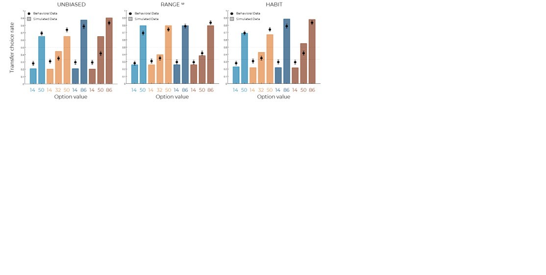
Model predictions of the UNBIASED (left), RANGEw (middle) and HABIT (right).
Simulated data in the transfer phase were obtained with the best-fitting parameters, optimized on all four contexts of the learning phase.
Author response image 5
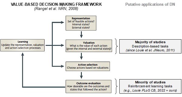
Value-based decision-making framework (as depicted by Rangel et al.) and where DN normalization has been traditionally (“Valuation”) and recently (“Outcome evaluation”) applied.
Author response image 6
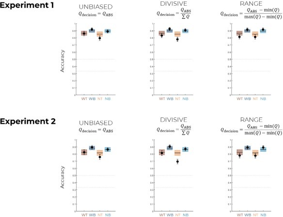
Participants’ accuracy (colored rectangles) and model simulations (black dots) in each condition of the learning phase.
Author response image 7
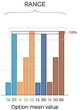
For the sake of completeness we show again here the two-learning rates-induced discrepancy between the preferences in N86/N50 and W86/W50.
Tables
Table 1
Experimental design.
Each version of each experiment was composed of four different learning contexts. Results of Experiments 1 and 3 are presented in the main text; results of Experiment 2 are presented in Figure 2—figure supplement 2. Entries inside square brackets represent the mean outcomes for the lowest, mid (when applicable), and highest value option in a given context. Concerning ‘forced choices,’ ‘unary’ refers to situations where only one option is available and the participants cannot make a choice; ‘binary’ refers to situations where the participant can choose between two out of three options (the high-value option cannot be chosen).
| N | Learning contexts | N forced choices(type / feedback) | ||||||
|---|---|---|---|---|---|---|---|---|
| [14,50] | [14,32,50] | [50,86] | [50,68,86] | [14,86] | [14,50,86] | |||
| Experiment 1a | 50 | X | X | X | X | 0 | ||
| Experiment 1b | 50 | X | X | X | X | 50 (unary / complete) | ||
| Experiment 1 | 50 | X | X | X | X | 50 (unary / partial) | ||
| Experiment 2a | 50 | X | X | X | X | 0 | ||
| Experiment 2b | 50 | X | X | X | X | 50 (unary / complete) | ||
| Experiment 2c | 50 | X | X | X | X | 50 (unary / partial) | ||
| Experiment 3a | 100 | X | X | 90 (binary / complete) | ||||
| Experiment 3b | 100 | X | X | 135 (binary / complete) | ||||
Table 2
Quantitative model comparison in Experiments 1 and 2.
Values reported here represent mean ± SD and median of out-of-sample log-likelihood for each model.
| Model | Experiment 1 (N = 150)Out-of-sample log-likelihood | Experiment 2 (N = 150s)Out-of-sample log-likelihood | ||
|---|---|---|---|---|
| Mean ± SD | Median | Mean ± SD | Median | |
| UNBIASED | –275.31 ± 268.75 | –162.53 | –227.24 ± 269.72 | –125.40 |
| DIVISIVE | –143.38 ± 70.40 | –124.91 | –159.89 ± 65.20 | –141.07 |
| RANGE | –116.72 ± 57.91 | –109.23 | –109.71 ± 43.91 | –106.83 |
| RANGE (ω) | –97.70 ± 55.52 | –78.73 | –91.99 ± 37.79 | –79.57 |
Additional files
Download links
A two-part list of links to download the article, or parts of the article, in various formats.
Downloads (link to download the article as PDF)
Open citations (links to open the citations from this article in various online reference manager services)
Cite this article (links to download the citations from this article in formats compatible with various reference manager tools)
The functional form of value normalization in human reinforcement learning
eLife 12:e83891.
https://doi.org/10.7554/eLife.83891


