Disruption of awake sharp-wave ripples does not affect memorization of locations in repeated-acquisition spatial memory tasks
- KU Leuven, Department of Physics and Astronomy, Soft Matter and Biophysics, Belgium
- NERF-NeuroElectronics Research Flanders, Kloosterman Lab, Belgium
- KU Leuven, Faculty of Psychology & Educational Sciences, Belgium
Figures
Figure 1 with 1 supplement
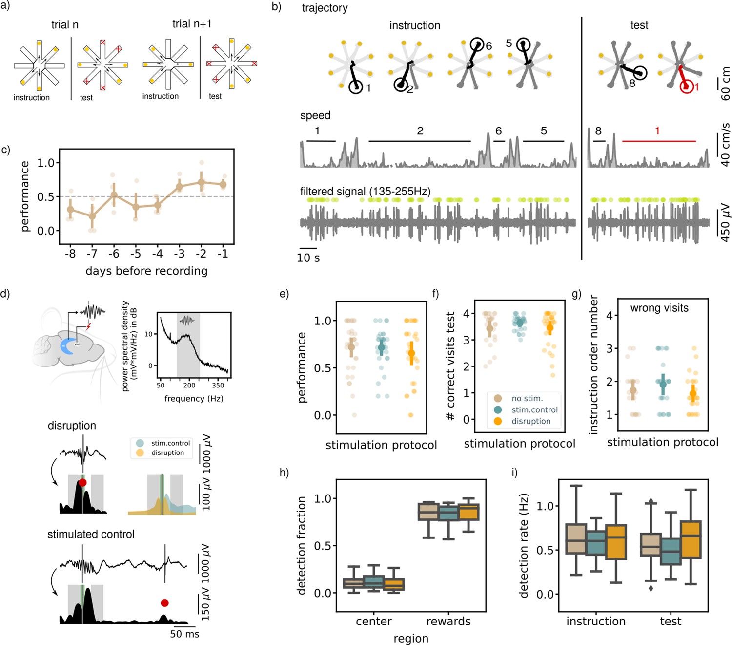
Executing a non-match-to-sample (NMTS) task is not awake SWR dependent.
(a) A schematic illustration of the setup used for the behavior. In a NMTS task all eight arms are rewarded but only four can be collected in the instruction phase and the rest needs to be collected in the test phase without an error. (b) Trajectory, speed and filtered LFP for an example trial. Red trajectory indicates a wrong visit, yellow dot a to be collected reward and the green dot an online ripple detection. (c) The learning curve over pretraining days for all animals (N=5) showing the average trial performance in a session. The dashed line indicates the learning criteria (small dots; results for individual animals, large dots; mean and 99% CI). (d) (top) Illustration showing the recording (HC) and stimulation (VHC) sites and a power spectral density of an example control session considering only the immobility periods (speed <5 cm/s). The grey shaded area indicates the chosen frequency range to filter the LFP before ripple detection. (bottom) Example LFP and envelope traces of a disrupted and delayed stimulated (bottom) ripple. The small grey line indicates the time of detection, the red dot the point of stimulation. The green shaded area covers the window in which the stimulation artifact was removed and the grey shaded areas indicate the time windows used to compare the ripple envelope before and after ripple detection. The top right shows the average envelope of all disrupted and delay stimulated ripples in one example session. (e) The average trial performance in a session per stimulation protocol (no stim: n=169, stim. control: n=155 and disruption: n=148). (f) Same as (e) but showing the number of visits in the test phase. (g) The instruction phase order number of the wrongly visited arm per stimulation protocol. Only wrong trials are considered. (no stim: n=47, stim. control: n=42and disruption: n=47). For visualization purpose each small dot in e, fand g represents a session average. The large dots represent the mean and 99%CI per condition. (h) The fraction of ripple detections during the trials on the rewards and central platforms. The small remaining fraction of detections happened on the arms. (i) The ripple detection rate during the instruction and test phase of the trials, considering only periods of immobility (speed <5 cm/s). In h and i the box shows the quartiles of the dataset while the whiskers extend to show the rest of the distribution. Outliers (defined using the inter-quartile range) are shown using a diamond marker. See also Figure 1—figure supplement 1.
Figure 1—figure supplement 1
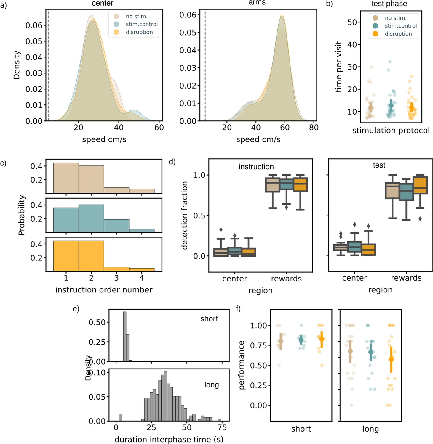
Additional behavioral analyses NMTS task show no effect of ripple disruption.
(a) Distribution of the average run speed on the central platform and maze arms for each stimulation protocol. The dashed line indicates the threshold used to determine immobility periods (5 cm/s). Running speed disruption: arms 54.02 cm/s [49.71,56.97], center 28.66 cm/s [26.03,31.84]. Running speed stim.control: arms 53.24 cm/s [47.93,56.45], center 28.39 cm/s [25.86,32.23]. Running speed no stim.: arms 53.09 cm/s [48.32,56.68], center 28.67 cm/s [26.37,31.51]. There is no significant difference due to ripple disruption: Kruskal-Wallis test, arms H=0.09, p=0.96, center H=0.42, p=0.81. (b) The average time per visit in the test phase of a trial per stimulation protocol: disruption 11.23 s [10.32,12.54], stim.control 11.64 s [10.69,12.96], no stim. 10.03 s [9.30,11.35]; Kruskal-Wallis test: H=12.19, p=0.0023 (no stim: n=169, stim. control: n=155 and disruption: n=148). (c) The distribution of the instruction order number for the incorrectly visit arm in incorrect trials, for all three stimulation protocols (no stim: n=47, stim. control: n=42and disruption: n=47). (d) The fraction of ripple detections during the instruction and test phase on the reward and central platforms. Fraction detections instruction phase at reward platforms: disruption 0.86 [0.79,0.91], stim.control 0.87 [0.81,0.91], no stim. 0.88 [0.82,0.92]. Fraction detections instruction phase at central platform: disruption 0.05 [0.03,0.09], stim.control 0.07 [0.05,0.11], no stim. 0.06 [0.03,0.10]. Fraction detections test phase at reward platforms: disruption 0.85 [0.77,0.90], stim.control 0.78 [0.72,0.84], no stim. 0.80 [0.74,0.86]. Fraction detections test phase at central platform: disruption 0.09 [0.06,0.15], stim.control 0.12 [0.08,0.16], no stim. 0.10 [0.08,0.14]. The reward bias is not significantly different between stimulation protocols: Kruskal-Wallis test, instruction: H=0.43, p=0.8, test: H=4.02, p=0.13. The box shows the quartiles of the dataset while the whiskers extend to show the rest of the distribution. Outliers (defined using the inter-quartile range) are shown using a diamond marker. (e) The distributions for the time between instruction and test phase, long 35.44 s [33.84,37.08], short 7.27 s [7.06,8.22]; Mann-Whitney test: U=920.00, p=8.2 × 10⁻²⁷. (f) The average trial performance per stimulation protocol in sessions with a short (no stim: n=80, stim. control: n=62 and disruption: n=56) or long (no stim: n=89, stim. control: n=93 and disruption: n=92) interphase delay. Performance long delay: Kruskal-Wallis test: H=1.04, p=0.59. Performance short delay: Kruskal-Wallis test: H=0.15, p=0.93. Statistics for the number of correct visits (not shown), long delay: disruption 3.39 [3.08,3.59], stim.control 3.59 [3.38,3.73], no stim. 3.34 [2.96,3.60]; H=1.46, p=0.48. Number of correct visits, short delay: disruption 3.73 [3.31,3.89], stim.control 3.76 [3.35,3.89], no stim. 3.65 [3.26,3.84]; H=0.21, p=0.9. In b and f each small dot represents a session average for visualization purpose. The large dots represent the mean and 99%CI per condition.
Figure 2 with 1 supplement
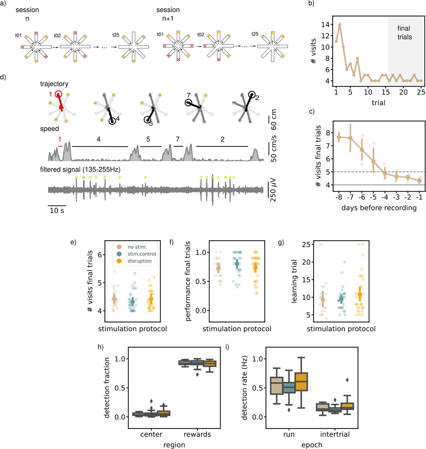
Executing a match-to-sample task (MTS) is not hippocampal ripple dependent.
(a) A schematic illustration of the setup used for the behavior. In an MTS task only four of the eight arms are rewarded. (b) Learning curve of one example session showing the total number of visits in each trial. (c) The learning curve over pretraining days for all animals (N=5) showing the average number of visits in the final trials per session (small dots; results for individual animals, large dots; mean and 99% CI over animals). The dashed line indicates the learning criteria, the solid line the perfect performance. (d) Trajectory, speed and filtered LFP for an example trial. Red trajectory indicates a wrong visit, yellow dot a to-be-collected reward and the green dot an online ripple detection. (e) The average number of visits in the final trials per stimulation protocol. (f) The average performance (binary quantification) in the final visits per stimulation protocol. (g) The learning trial per stimulation protocol. In e, (f, and g) small dots represent results for individual sessions (disruption: n=32, stim.control: n=31, no stim.: n=19), large dots reflect the mean and 99%CI per stimulation protocol. (h) The fraction of ripple detections during the trials on the rewards and central platforms. The small remaining fraction of detections happened on the arms. (i) The ripple detection rate during trials considering only periods of immobility (speed <5 cm/s) and during inter-trial epochs. In h and i the box shows the quartiles of the dataset while the whiskers extend to show the rest of the distribution. Outliers (defined using the inter-quartile range) are shown using a diamond marker. See also Figure 2—figure supplement 1.
Figure 2—figure supplement 1
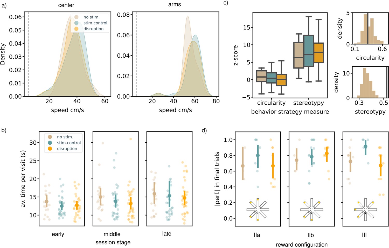
Additional behavioral analyses MTS task show no effect of ripple disruption.
(a) Distribution of the average run speed on the central platform and maze arms for each stimulation protocol. The dashed line indicates the threshold used to determine immobility periods (5 cm/s). The running speed is significantly lower on the central platform than in the arms for all three stimulation conditions. Running speed disruption condition: center 36.42 cm/s [33.13,39.02], arms 57.15 cm/s [52.20,59.65]; Mann-Whitney test: U=43.00, p=1.3 × 10⁻¹⁰. Running speed stim.control condition: center 38.06 cm/s [34.54,40.62], arms 58.12 cm/s [52.69,60.62]; Mann-Whitney test: U=30.00, p=1 × 10⁻¹⁰. Running speed no stim. condition: center 36.78 cm/s [33.72,41.01], arms 55.95 cm/s [53.39,59.50]; Mann-Whitney test: U=2.00, p=1 × 10⁻⁶. The running speed for each maze region is not significantly different across stimulation protocols (Kruskal-Wallis test, center: H=2.03, p=0.36, arms: H=4.14, p=0.13). (b) The average time per visit in the early (1-8), middle (9-17), and late (18-25) trials of a session is not significantly different in the disruption vs. control sessions (disruption: n=32, stim.control: n=31, no stim.: n=19). Time per visit in early trials, disruption 12.71 s [11.51,14.11], stim.control 12.49 s [11.41,14.02], no stim. 13.75 s [11.88,15.88]; Kruskal-Wallis test: H=1.74, p=0.42. Time per visit in middle trials, disruption 13.15 s [11.62,16.20], stim.control 13.83 s [12.01,16.53], no stim. 15.00 s [12.87,19.01]; Kruskal-Wallis test: H=2.25, p=0.32. Time per visit in late trials, disruption 14.73 s [12.77,17.00], stim.control 15.31 s [12.42,21.68], no stim. 15.87 s [13.04,20.90]; Kruskal-Wallis test: H=1.52, p=0.47. (c) Left: distributions of the per-session z-scores for the fraction of (counter)clockwise trials (circularity) and stereotypy index. Z-scores are computed with respect to shuffle distributions (see methods) and do not change due to ripple disruption (Kruskal-Wallis test, circularity: H=0.37, p=0.83, stereotypy: H=0.85, p=0.65). The box shows the quartiles of the dataset while the whiskers extend to show the rest of the distribution. Right: example shuffle distribution (gray) and actual value (black line) for circularity and stereotypy in single session. (d) The average performance in the final trials of a session, split by arm configuration. Configuration IIa: Kruskal-Wallis test: H=1.58, p=0.45 (disruption: n=8, stim.control: n=8, no stim.: n=3) . Configuration IIb: Kruskal-Wallis test: H=1.13, p=0.57 (disruption: n=11, stim.control: n=15, no stim.: n=5). Configuration III: Kruskal-Wallis test: H=6.21, p=0.045 (disruption: n=11, stim.control: n=6, no stim.: n=9). Average number of visits in final trials, configuration IIa: disruption 4.73 [4.26,5.51], stim.control 4.26 [4.06,4.62], no stim. 4.77 [4.40,5.40]; Kruskal-Wallis test: H=4.08, p=0.13. Configuration IIb: disruption 4.26 [4.11,4.47], stim.control 4.41 [4.19,4.73], no stim. 4.38 [4.08,4.80]; Kruskal-Wallis test: H=0.87, p=0.65. Configuration III: disruption 4.42 [4.22,4.67], stim.control 4.10 [4.00,4.23], no stim. 4.40 [4.18,4.68]; H=6.07, p=0.048. Learning trial, configuration IIa: disruption 10.38 [7.25,14.88], stim.control 10.00 [7.38,15.88], no stim. 14.00 [6.00,25.00]; Kruskal-Wallis test: H=0.40, p=0.82. Configuration IIb: disruption 12.18 [8.09,18.27], stim.control 9.00 [7.53,10.07], no stim. 8.80 [5.80,12.00]; Kruskal-Wallis test: H=0.71, p=0.7. Configuration III: disruption 10.27 [7.36,16.66], stim.control 9.83 [6.33,14.67], no stim. 9.00 [6.33,11.44]; Kruskal-Wallis test: H=0.07, p=0.96. In b and d small dots represent results for individual sessions , large dots reflect the mean and 99%CI per stimulation protocol.
Figure 3 with 1 supplement
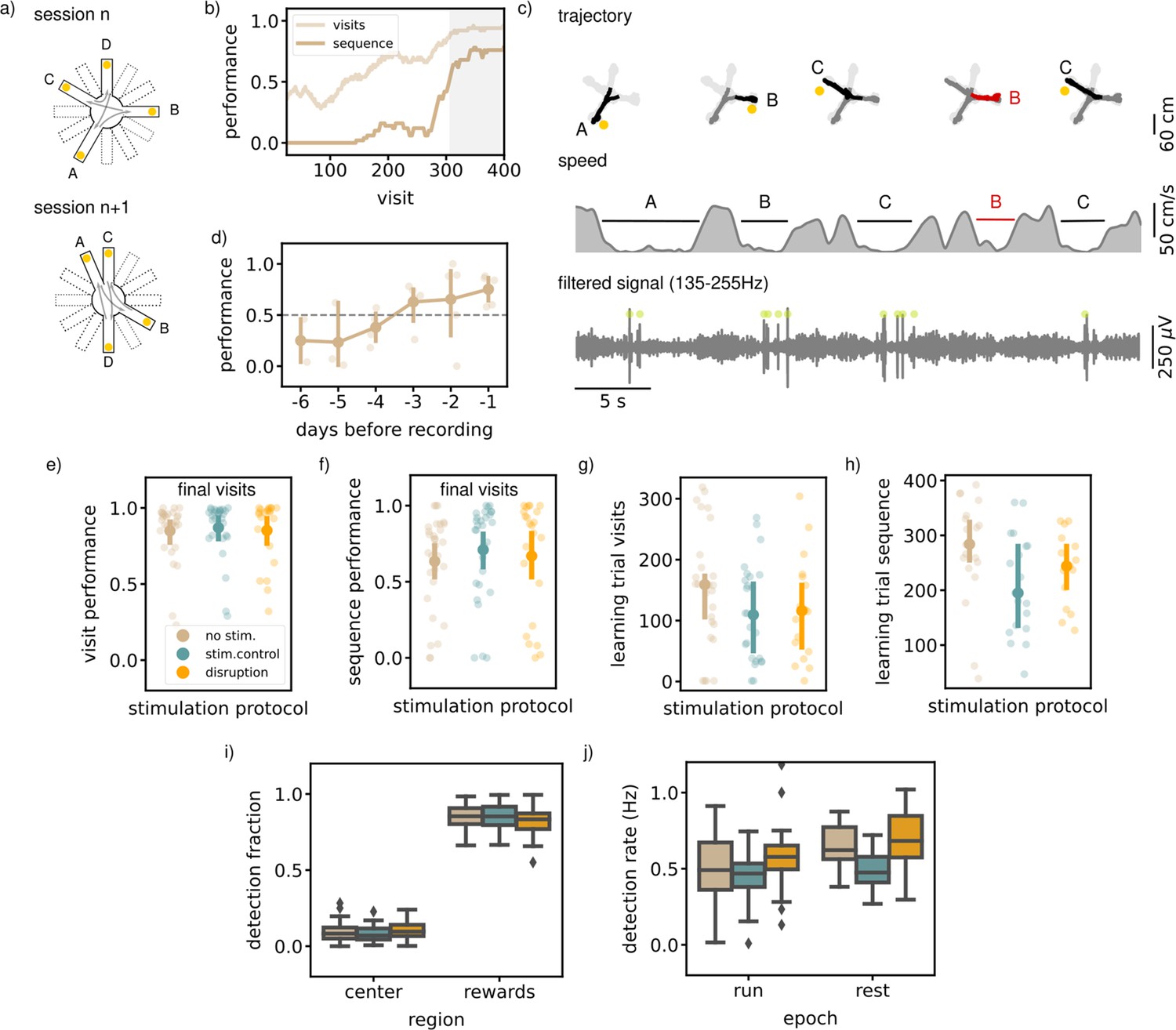
Executing a sequential (SEQ) spatial memory task is not hippocampal ripple dependent.
(a) A schematic illustration of the setup used for the behavior. In a SEQ task only four of twelve possible arms are present. Reward is delivered when arms are visited in the correct order. (b) Learning curves of one example session showing the visit performance and sequence performance over visits, both visualized using a moving average with N=50. (c) Trajectory, speed and filtered LFP for five visits in an example session. Red trajectory indicates a wrong visit, yellow dot a to be collected reward and the green dot an online ripple detection. (d) The learning curve over pretraining days for all animals (N=5) showing the average sequence performance in the final 100 visits in a session. The dashed line indicates the learning criteria (small dots; result per animal, large dots: mean and 99% CI). (e) The average visit performance over the final visits of a session per stimulation protocol. One small dot represents one session (no stim: n=31, stim. control: n=29 and disruption: n=23) and the large dot the mean and 99%CI. (f) Same as (e) but showing the average sequence performance over the final visits of a session. (g) The visit learning trial of sessions per stimulation protocol defined using the smoothed learning curve of the visit performance (see methods). Only session where learning criteria was met within 400 visits are included. (h) Same as (g) but showing the sequence learning trial computed using the smoothed learning curve of the sequence performance. (i) The fraction of ripple detections during the trials on the rewards and central platforms. The small remaining fraction of detections happened on the arms. (j) The ripple detection rate during run on the maze, considering only periods of immobility (speed <5 cm/s), and during rest epochs in the sleep box. In i and j the box shows the quartiles of the dataset while the whiskers extend to show the rest of the distribution. Outliers (defined using the inter-quartile range) are shown using a diamond marker.See also Figure 3—figure supplement 1.
Figure 3—figure supplement 1

Additional behavioral analyses SEQ task show no effect of ripple disruption.
(a) Distribution of the average running speed on the central platform and maze arms for each stimulation protocol. The dashed line indicates the threshold used to determine immobility periods (5 cm/s). Running speed in center: disruption 46.01 cm/s [42.55,49.30], stim.control 47.56 cm/s [42.90,51.75], no stim. 46.93 cm/s [44.89,48.88]; Kruskal-Wallis test: H=1.20, p=0.55. Run speed in arms: disruption 47.49 cm/s [45.17,49.55], stim.control 48.43 cm/s [44.68,50.98], no stim. 48.29 cm/s [47.03,49.35]; Kruskal-Wallis test: H=1.79, p=0.41. (b) The average time per visit in a session per stimulation protocol: disruption 7.72 s [7.67,7.79], stim.control 7.73 s [7.68,7.78], no stim. 7.50 s [7.46,7.53]; Kruskal-Wallis test: H=0.77, p=0.68 (no stim: n=31, stim. control: n=29 and disruption: n=23) (c) Learning curves for individual transitions in one example session. The dashed line indicates the learning criterium, the tick marks at the top indicate correct visits. (d) Distribution of transition learning trials for all sessions in each stimulation protocol, Kruskal-Wallis test: H=10.62, p=0.0049. Post-hoc tests: disruption - stim.control, U=3946.00, p=0.43; disruption - no stim., U=4801.50, p=0.041; stim.control - no stim., U=9782.50, p=0.0021. (e) The learning trial difference for each session, defined as the difference between the learning trial of the slowest and fastest learned transition. Disruption: 38.95 [26.15,55.73]; stim.control: 38.30 [30.26,49.30]; no stim.: 49.31 [36.28,62.97]; Kruskal-Wallis test: H=3.10, p=0.21. Only sessions in which at least two transitions were learned are included (disruption: N=20, stim.control: N=27, no stim.: N=29). In b and e, a small dot represents one session and the large dot represents the mean and 99%CI.
Figure 4 with 2 supplements
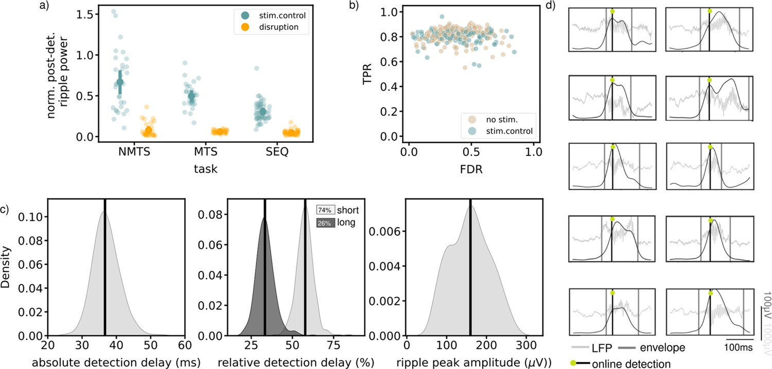
Available quantifications indicate accurate ripple detection and disruption.
(a) Normalized post-detection ripple power for all tree tasks in run epochs (NMTS: disruption: n_trials=148, stim.control: n_trials=155 , MTS: disruption: n_sessions=31, stim.control: n_sessions=31 , SEQ: disruption: n_sessions=23, stim.control: n_sessions=29). A small dot represents the average over one session, the large dots represent the mean and 99%CI. (b) True positive rate versus False discovery rate for all tasks. One dot represents the average over one session. (c) The absolute detection delays (left), relative detection delays for both the short (74% of all ripples) and long ripples (26% of all ripples) (middle) and ripple peak amplitude for all epochs of all tasks, considering the no stim. and stim.control epochs. (d) Example online detected ripples that were also detected offline (true positive) from five different animals. Grey vertical lines indicate the start and end of the ripple. See also Figure 4—figure supplements 1 and 2.
Figure 4—figure supplement 1
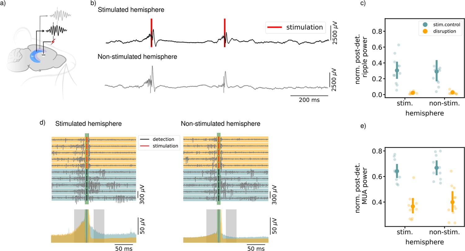
Hippocampal ripples are disrupted bilaterally.
(a) Illustration showing the bilateral recording (HC) sites and stimulation (VHC) site. (b) Example LFP traces of disrupted ripples in the stimulated hemisphere (top) and non-stimulated hemisphere (bottom). (c) Normalized post-detection ripple power for stimulated and non-stimulated hemisphere in disruption and stimulated control conditions (Mann-Whitney test, stimulated hemisphere: U=121.00, p=4.1 × 10⁻⁵, non-stimulated hemisphere: U=118.00, p=9.1 × 10⁻⁵). Each small dot represents the average over one session, the large dots represent the mean and 99% CI. Quantification was performed on 11 sessions in total for each stimulation protocol that were acquired from three animals (on average, 214 ripples per session were analyzed). (d) Top: example MUA traces from the stimulated (left) and non-stimulated (right) hemispheres for both disruption (yellow) and stimulated control (green) conditions. Red/black vertical lines indicate the time of ripple detection and VHC stimulation, respectively. A short window around the time of the detection/stimulation (shaded green) that contains the stimulation artefact was excluded from the analysis. Bottom: average MUA power across all ripples for disruption (yellow) and stimulated control (blue) conditions. The grey shaded areas indicate the time windows that were used to compare the MUA power before and after ripple detection. (e) Normalized post-detection MUA power for stimulated and non-stimulated hemispheres in disruption and stimulated control conditions for all sessions (Mann-Whitney test, stimulated hemisphere: U=118.00, p=9.1 × 10⁻⁵, non-stimulated hemisphere: U=116.00, p=0.00015). The small dots represent the average over one session, the large dots represent the mean and 99% CI. Animals rested in a sleep box during the recordings.
Figure 4—figure supplement 2
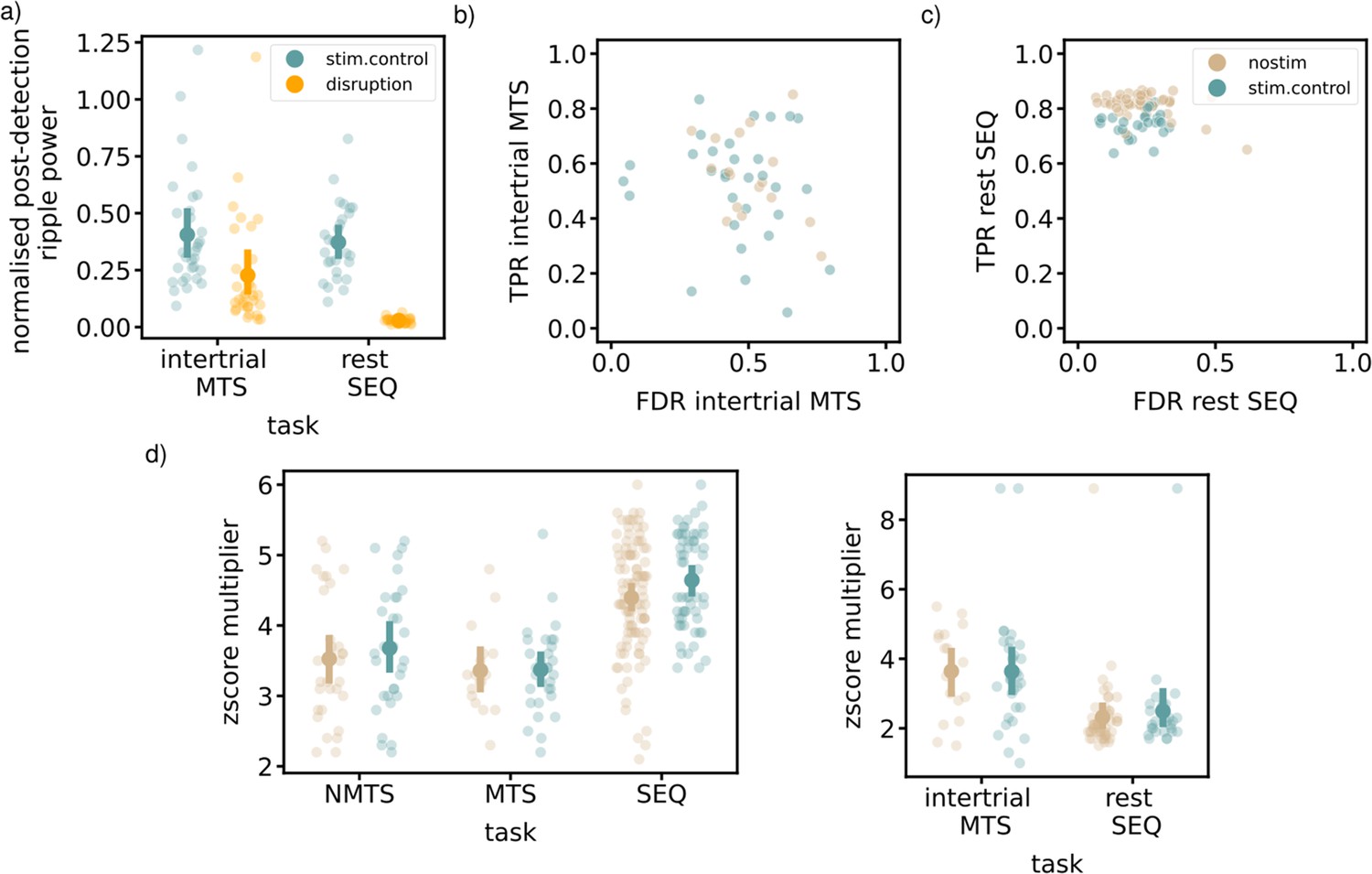
Quantification of ripple detection and disruption in rest epochs.
Tables
Table 1
Overview animals NMTS.
| Animal | N sessions | distruption trials | stim.control trials | no stim. trials |
|---|---|---|---|---|
| LD06 | 8 | 34 | 32 | 24 |
| LD07 | 7 | 27 | 30 | 29 |
| LD08 | 7 | 31 | 31 | 32 |
| LD12 | 6 | 40 | 39 | 43 |
| LD13 | 4 | 15 | 21 | 24 |
| Total | 32 | 147 | 153 | 152 |
Table 2
Overview animals MTS.
| Animals | Disruption sessions | Stim.control sessions | No stim sessions |
|---|---|---|---|
| LD10 | 4 | 3 | 1 |
| LD11 | 3 | 2 | 3 |
| LD14 | 9 | 10 | 6 |
| LD21 | 8 | 8 | 4 |
| LD22 | 7 | 8 | 3 |
| Total | 31 | 31 | 17 |
Table 3
Overview animals SEQ.
| Animals | Disruption sessions | Stim. Control sessions | No stim. sessions |
|---|---|---|---|
| LD53 | 7 | 7 | 7 |
| LD56 | 8 | 7 | 6 |
| LD57 | 5 | 6 | 6 |
| LD58 | 5 | 5 | 6 |
| LD60 | 6 | 4 | 4 |
| Total | 31 | 29 | 29 |
Table 4
Overview animals bilateral recordings.
| Animals | Disruption sessions | Stim. Control sessions |
|---|---|---|
| ST3 | 3 | 3 |
| ST4 | 4 | 4 |
| ST5 | 4 | 4 |
| Total | 11 | 11 |
Additional files
Download links
A two-part list of links to download the article, or parts of the article, in various formats.
Downloads (link to download the article as PDF)
Open citations (links to open the citations from this article in various online reference manager services)
Cite this article (links to download the citations from this article in formats compatible with various reference manager tools)
Disruption of awake sharp-wave ripples does not affect memorization of locations in repeated-acquisition spatial memory tasks
eLife 13:e84004.
https://doi.org/10.7554/eLife.84004


