Using light and X-ray scattering to untangle complex neuronal orientations and validate diffusion MRI
- Department of Imaging Physics, Faculty of Applied Sciences, Delft University of Technology, Netherlands
- Institute of Neuroscience and Medicine (INM-1), Forschungszentrum Jülich GmbH, Germany
- Stanford Synchrotron Radiation Lightsource, SLAC National Accelerator Laboratory, United States
- Department of Radiology, Stanford School of Medicine, United States
Figures
Figure 1
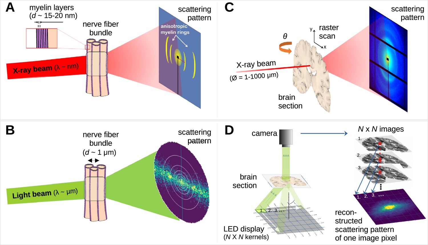
Comparison of X-ray scattering (top) and light scattering (bottom) for analyzing nerve fiber structures.
(A) Principle of X-ray scattering on a nerve fiber bundle, resulting in a ring at a radial position corresponding to myelin’s periodicity, strongest perpendicular to the in-plane fiber orientation. (B) Principle of light scattering on a nerve fiber bundle, which similarly yields scattered photons perpendicular to the in-plane fiber orientation. (C) Schematic drawing of a 3D-scanning small-angle X-ray scattering (3D-sSAXS) measurement of a brain section, in which raster scanning at multiple angles allows reconstructing 3D fiber orientation distributions for each point of illumination. (D) Schematic drawing of a scattered light imaging (SLI) scatterometry measurement of a whole brain section (left) and reconstruction of a scattering pattern for one selected image pixel (right), which can be performed over the entire image simultaneously.
Figure 2 with 1 supplement
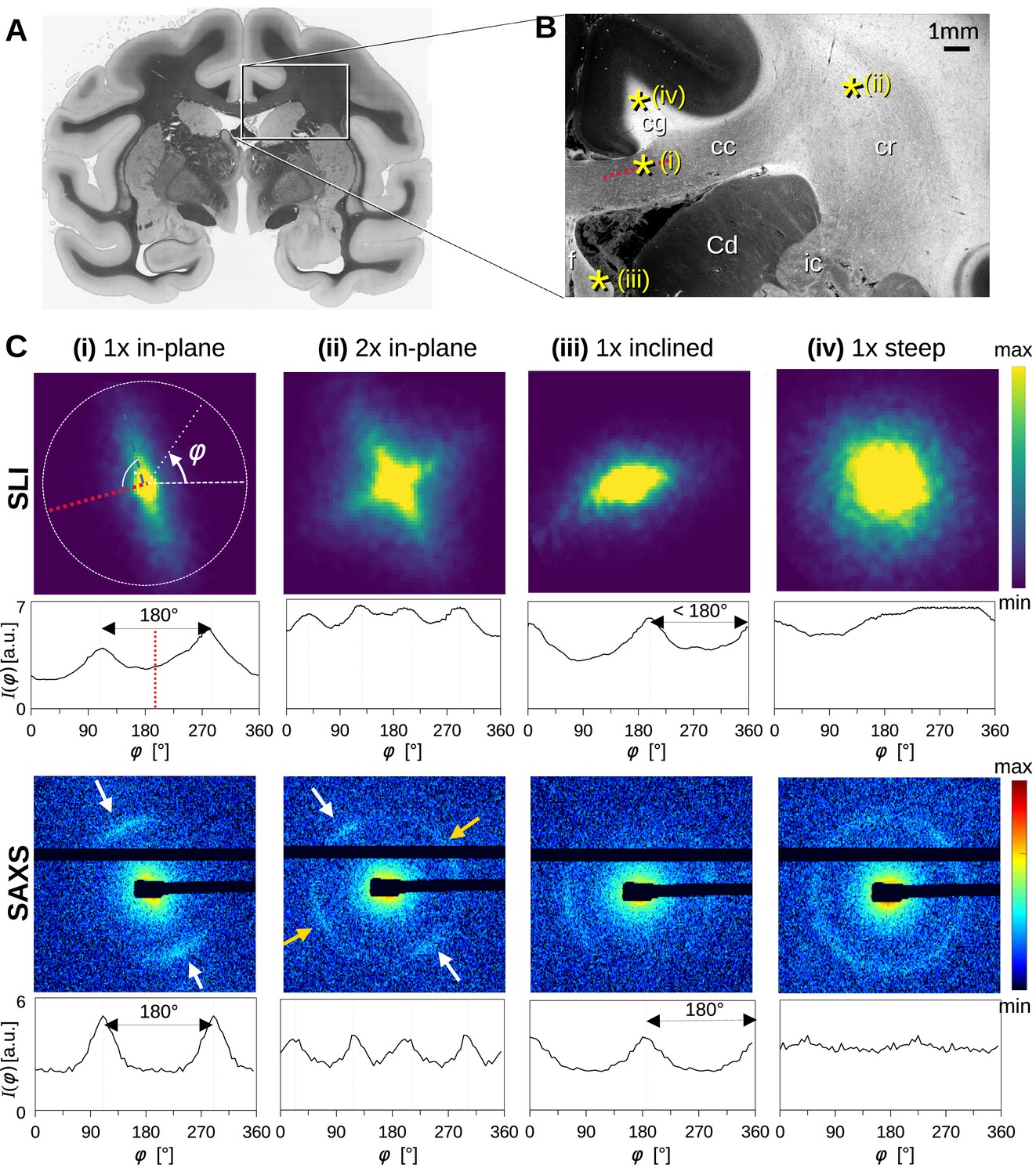
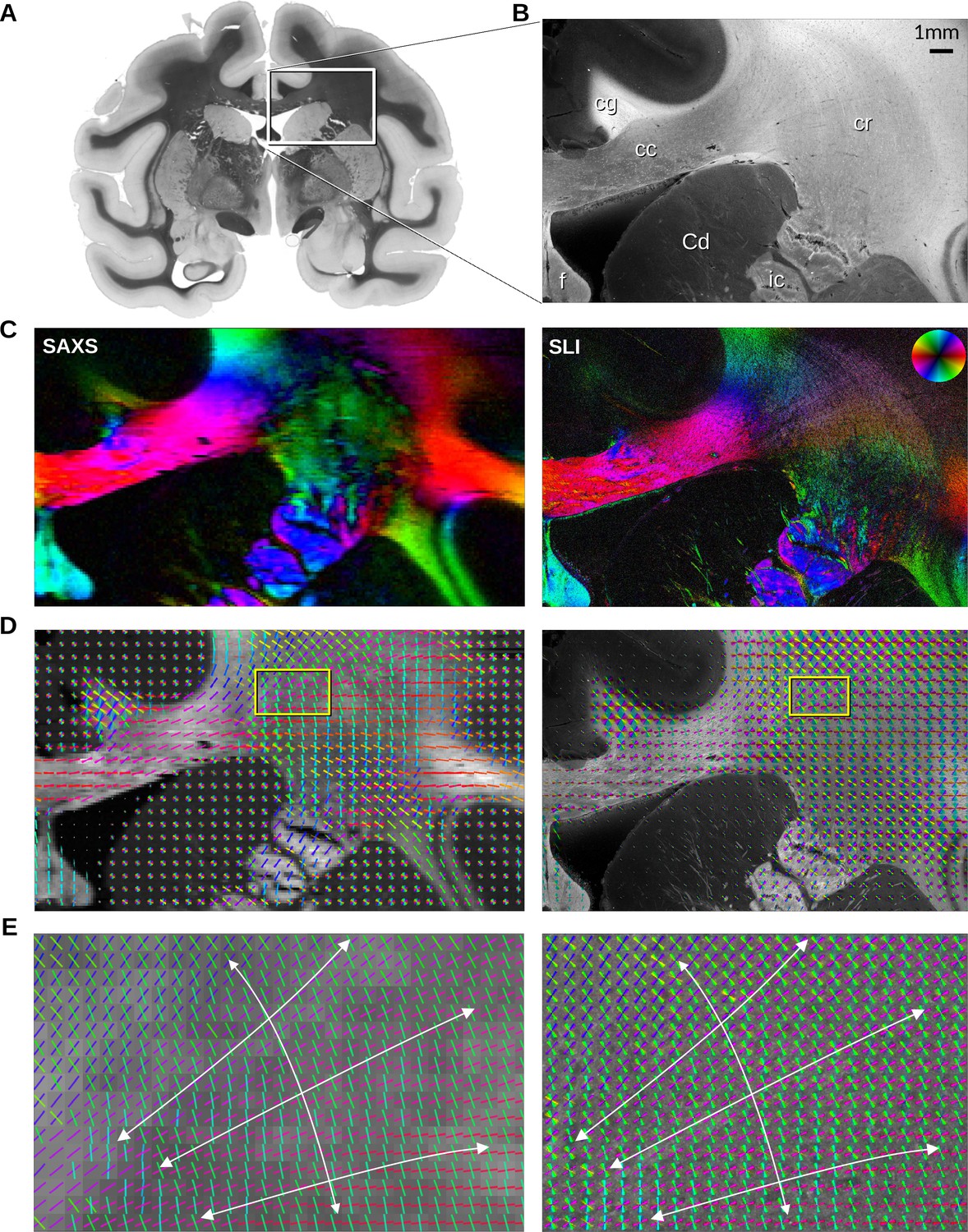
Scattering patterns obtained from scattered light imaging (SLI) scatterometry (px = 3 μm) and small-angle X-ray scattering (SAXS) (px = 100 μm) on a 60 μm-thick vervet monkey brain section at a coronal plane between the amygdala and hippocampus (section no. 511).
(A) Transmittance image of the whole brain section. (B) Average scattered light intensity of the investigated region (cc: corpus callosum, cr: corona radiata, cg: cingulum, Cd: caudate nucleus, f: fornix, ic: internal capsule). Yellow asterisks indicate the points corresponding to the scattering patterns in C. (C) Scattering patterns from SLI (top) and SAXS (bottom) with azimuthal profiles plotted beneath each pattern, obtained from the pixels indicated in B. (i) unidirectional in-plane fiber bundle in the corpus callosum, with peaks perpendicular to the fiber orientation (red dotted line), lying 180° apart, (ii) two in-plane crossing fiber bundles in the corona radiata, (iii) slightly inclined fiber bundle in the fornix, with SLI peaks <180° apart, and SAXS peaks 180° apart but with lower Bragg peak intensity, (iv) highly inclined fiber bundle in the cingulum, with no SLI azimuthal peak pair and almost isotropic SAXS myelin ring.
Figure 2—figure supplement 1
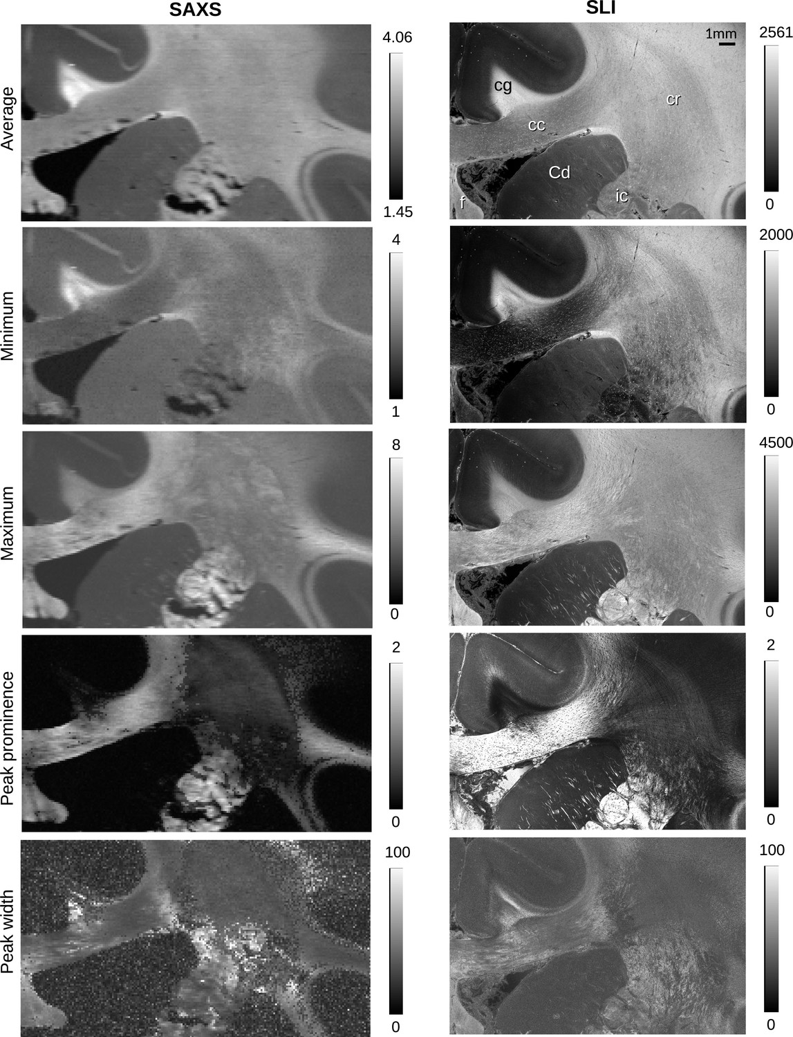
Parameter maps obtained from small-angle X-ray scattering (SAXS) and scattered light imaging (SLI) azimuthal profiles for vervet brain section no. 511.
The top images show the average, maximum, and minimum values of the azimuthal profiles for each image pixel. The lower images show the mean prominence and width of the peaks in the azimuthal profiles. The images show a similar behavior corresponding to the azimuthal profiles shown in Figure 2C: Out-of-plane nerve fibers in the cingulum yield high average scattered light intensities with small signal amplitude (max–min), small peak prominence, and large peak width. In-plane nerve fibers in the corpus callosum yield a large signal amplitude, high peak prominence, and small peak width. In-plane crossing nerve fibers in the corona radiata yield a smaller signal amplitude and less prominent peaks.
Figure 3 with 1 supplement
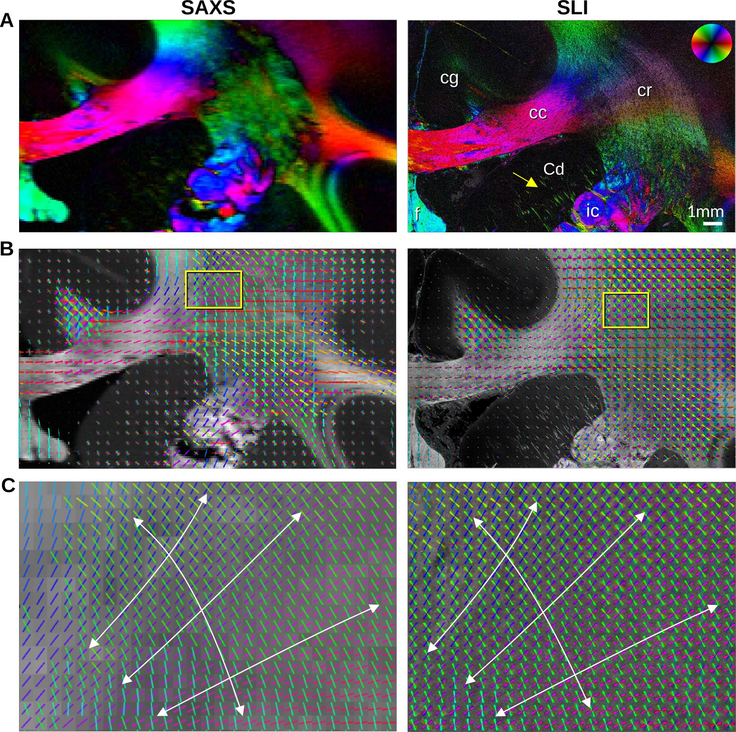
In-plane nerve fiber orientations from small-angle X-ray scattering (SAXS) and scattered light imaging (SLI) measurements of vervet monkey brain section no. 511.
(A) Fiber orientation maps showing the predominant fiber orientation for each image pixel in different colors (see the color wheel in the upper right corner): px = 100 μm (SAXS), px = 3 μm (SLI). (cc: corpus callosum, cr: corona radiata, cg: cingulum, Cd: caudate nucleus, f: fornix, ic: internal capsule). (B) Fiber orientations are displayed as colored lines for 5 × 5 px (SAXS) and 165 × 165 px (SLI) superimposed. The length of the lines is weighted by the averaged scattered light intensity in SAXS and SLI, respectively. (C) Enlarged region of the corona radiata, showing fiber orientations as colored lines for 1 × 1 px (SAXS) and 33 × 33 px (SLI) superimposed. The white arrows indicate the main stream of the computed fiber orientations.
Figure 3—figure supplement 1
In-plane fiber orientations from small-angle X-ray scattering (SAXS) and scattered light imaging (SLI) measurements of vervet brain section no. 501.
(A) Transmittance image of the whole section. (B) Average scattered light intensity of the investigated region (cc: corpus callosum, cr: corona radiata, cg: cingulum, Cd: caudate nucleus, f: fornix, ic: internal capsule). (C) Fiber orientation maps showing the predominant fiber orientation for each image pixel in different colors (see color wheel in upper right): px = 100 μm (SAXS), px = 3 μm (SLI). (D) Fiber orientations displayed as colored lines for 5 × 5 px (SAXS) and 165 × 165 px (SLI) superimposed. (E) Enlarged region of the corona radiata, showing fiber orientations as colored lines for 1 × 1 px (SAXS) and 33 × 33 px (SLI) superimposed. The white arrows indicate the overall course of the fiber vectors.
Figure 4 with 1 supplement
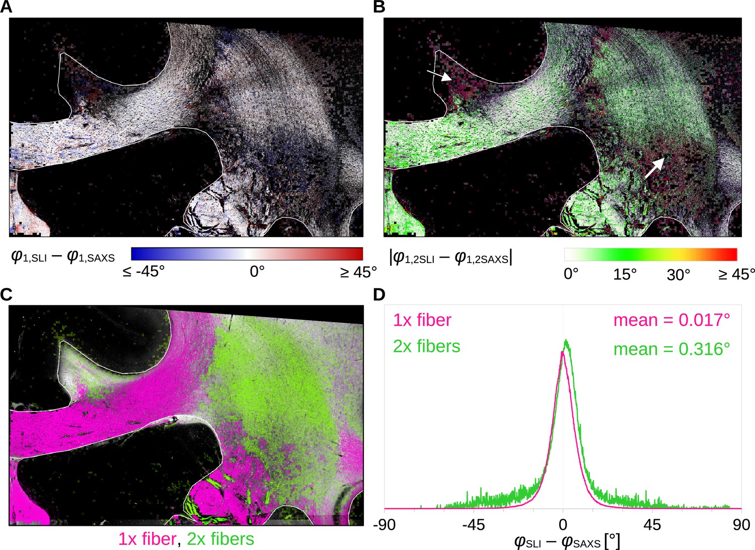
Angular difference between scattered light imaging (SLI) and small-angle X-ray scattering (SAXS) nerve fiber orientations (SLI – SAXS) for vervet monkey brain section no. 511.
For evaluation, the SAXS image was registered onto the SLI image (with 3 µm pixel size) and only regions where both techniques yield the same number of fiber orientations were considered. (A) Angular difference displayed for one of the maximum two predominating fiber orientations in each pixel. (B) Absolute angular difference displayed for each image pixel. (C) Regions with one or two fiber orientations for both methods (magenta = 1, green = 2 orientations). (D) Histograms showing the angular difference for pixels with one and two fiber orientations, evaluated in white matter regions excluding the fornix (see regions delineated by white lines in A-C).
Figure 4—figure supplement 1
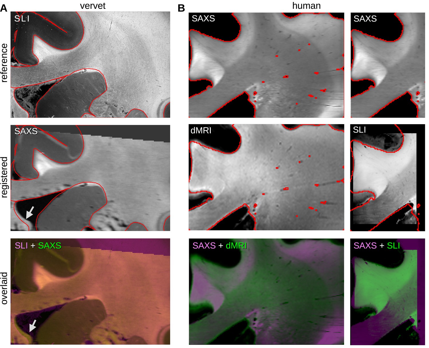
Quality of registration for vervet and human brain samples.
(A) Registration of small-angle X-ray scattering (SAXS) onto scattered light imaging (SLI) average intensity map for vervet brain section no. 511. The top and middle images show the SLI and registered SAXS average maps, respectively, the latter after linear transformation to align with SLI; the red outlines indicate the boundaries of gray and white matter in the SLI reference image. The bottom image shows the two modalities overlaid (SLI in blue violet, SAXS in green). The gray/white matter boundaries coincide (as the red outlines also show); only the fornix is slightly shifted (see white arrows) and was, therefore, manually evaluated (see text). (B) Registration of diffusion magnetic resonance imaging (dMRI) and SLI onto SAXS average map for the posterior human brain section no. 18. The top images show the SAXS average intensity map, the middle images show the registered dMRI map (scalar fiber orientation distribution obtained from the dwi2fod function of MRtrix) on the left, and the SLI average intensity map on the right; the red outlines indicate the boundaries of white matter in the SAXS reference image. The bottom images show the modalities overlaid (SAXS in blue violet, dMRI/SLI in green). The gray/white matter boundaries generally coincide.
Figure 5 with 5 supplements
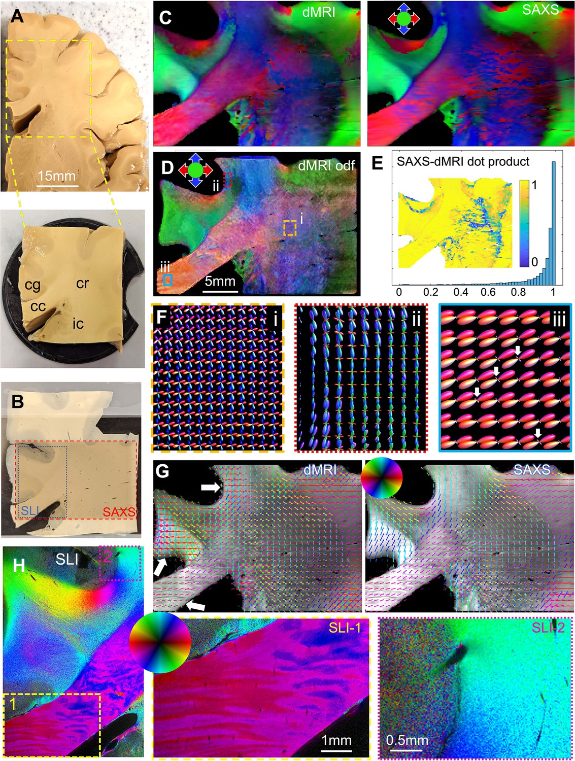
Diffusion magnetic resonance imaging (dMRI) measurement of a 3.5 × 3.5 × 1 cm³ human brain specimen (200 μm voxel size) in comparison to measurements with 3D-scanning SAXS (3D-sSAXS) (150 μm pixel size) and scattered light imaging (SLI) (3 μm pixel size) of a 80 μm-thick brain section.
(A) Human brain specimen; the bottom image shows the sample measured with dMRI (cc: corpus callosum, cg: cingulum, cr: corona radiata, ic: internal capsule). (B) Posterior brain section with regions measured by 3D-sSAXS (red rectangle) and SLI (blue rectangle). (C) Main 3D fiber orientations from dMRI (left) and 3D-sSAXS (right) for the brain section; dMRI was registered onto 3D-sSAXS (with 150 μm pixel size), see Figure 4—figure supplement 1B. (D) Orientation distribution functions from dMRI, with zoomed-in regions surrounded by rectangles shown in subfigure F. (E) Vector dot product of the dMRI and 3D-sSAXS main fiber orientations, as histogram and map of the studied area. (F) The enlarged regions from subfigure D show the fiber orientation distributions in the corona radiata (rectangle i, orange), a subcortical fiber bundle (rectangle ii, red), and the corpus callosum (rectangle iii, cyan). The fiber orientation distributions are almost identical to the ones shown here also when only high b-values are taken into account, Figure 5—figure supplement 4. (G) In-plane fiber orientation vectors for dMRI (left) and SAXS (right) superimposed on mean SAXS intensity. Vectors of 5 × 5 pixels are overlaid to enhance visibility. Zoomed-in images of the corona radiata region from both methods are shown in Figure 5—figure supplement 3C. (H) In-plane fiber orientations from SLI (multiple fiber orientations are displayed as multi-colored pixels), with zoomed-in areas in boxes (1) and (2). For better readability, fiber orientations in the gray matter are not shown in subfigures C-G.
Figure 5—figure supplement 1
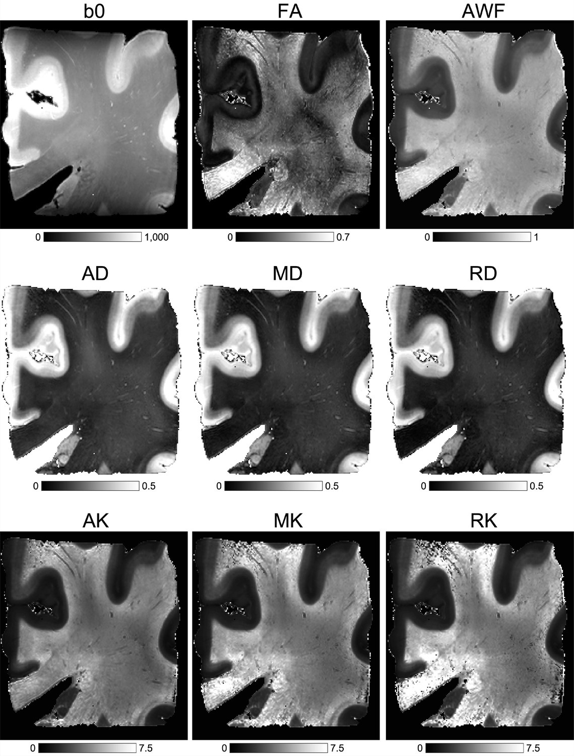
Anatomic (b0 – T2w) and diffusion MRI-based metrics for the human brain sample.
The images were calculated using the DESIGNER pipeline, which includes kurtosis and white matter tract integrity (WMTI) metrics: fractional anisotropy (FA), axonal water fraction (AWF), axial, mean, and radial diffusivity (AD, MD, RD), axial, mean, and radial kurtosis (AK, MK, RK).
Figure 5—figure supplement 2
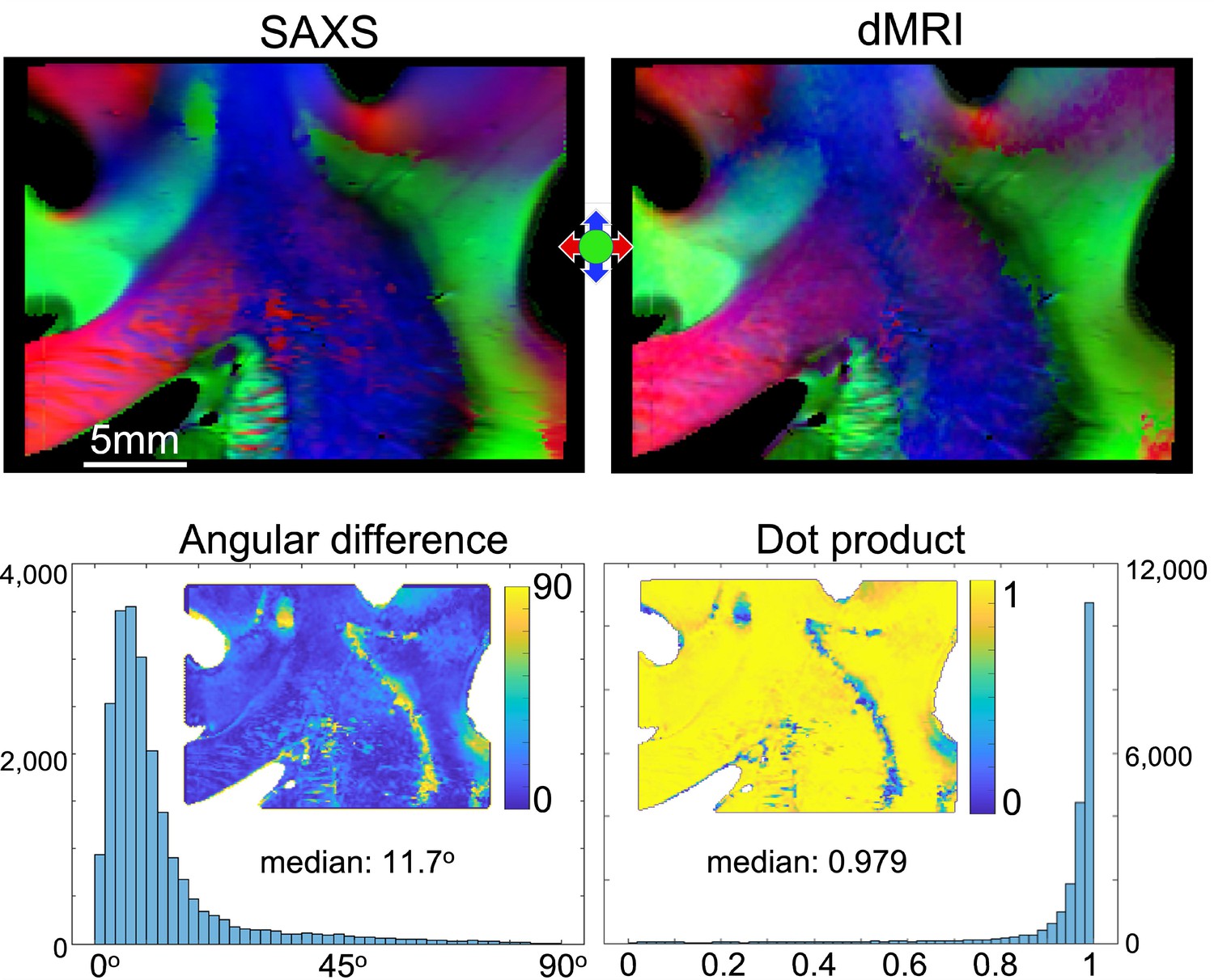
Small-angle X-ray scattering (SAXS)-diffusion magnetic resonance imaging (dMRI) comparison for the anterior human brain section no. 20.
The top row shows the 3-dimensional orientations of the fibers retrieved by 3D-scanning SAXS (3D-sSAXS) and dMRI, respectively. The dMRI image was upscaled and registered to the SAXS image (px = 150 µm). The bottom row quantifies the difference in the angles retrieved by the two methods. To the left, the absolute angular difference is plotted as a histogram and mapped on the section. To the right, the angular difference is quantified in the form of a dot product. The median angular difference found is 11.7o, which corresponds to a dot product of 0.970.
Figure 5—figure supplement 3
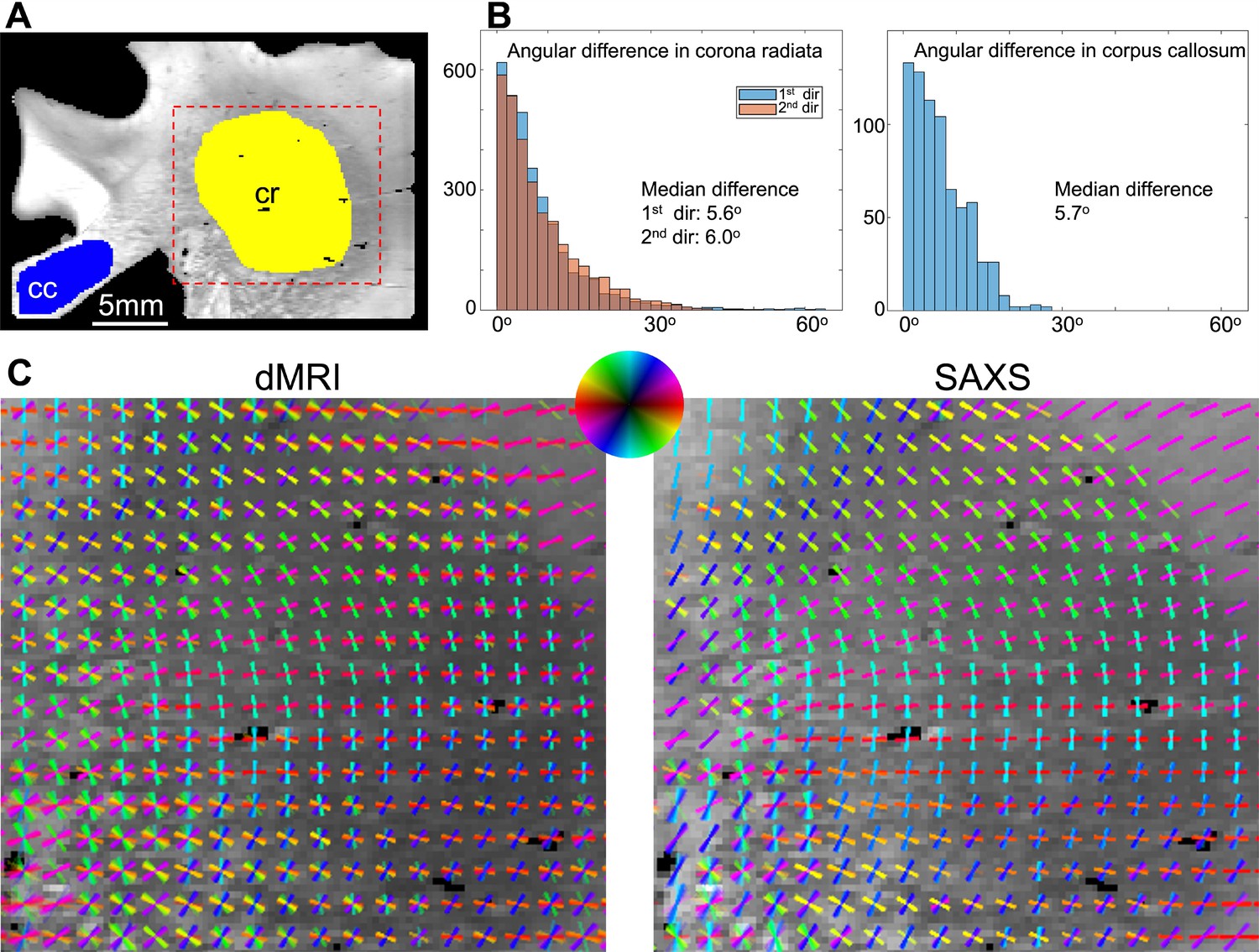
Quantifying in-plane angular differences between small-angle X-ray scattering (SAXS) and diffusion magnetic resonance imaging (dMRI) for the corpus callosum (cc) and corona radiata (cr) areas of the posterior human brain section no. 18.
(A) Map of the scattering intensity of the section, depicting the areas where quantification was performed. (B) Left, the histograms of the angular differences of the first and second fiber direction in the corona radiata are overlaid, showing very similar results (5.6° difference for the first direction, 6° for the second). Right, the same quantification for the corpus callosum area is shown (5.7° difference for the first direction; the second direction does not exist for SAXS in this region). (C) Zoom-in to the fiber orientations in the corona radiata, retrieved by dMRI and SAXS (orientations of 5 x 5 pixels are displayed on top of each other).
Figure 5—figure supplement 4
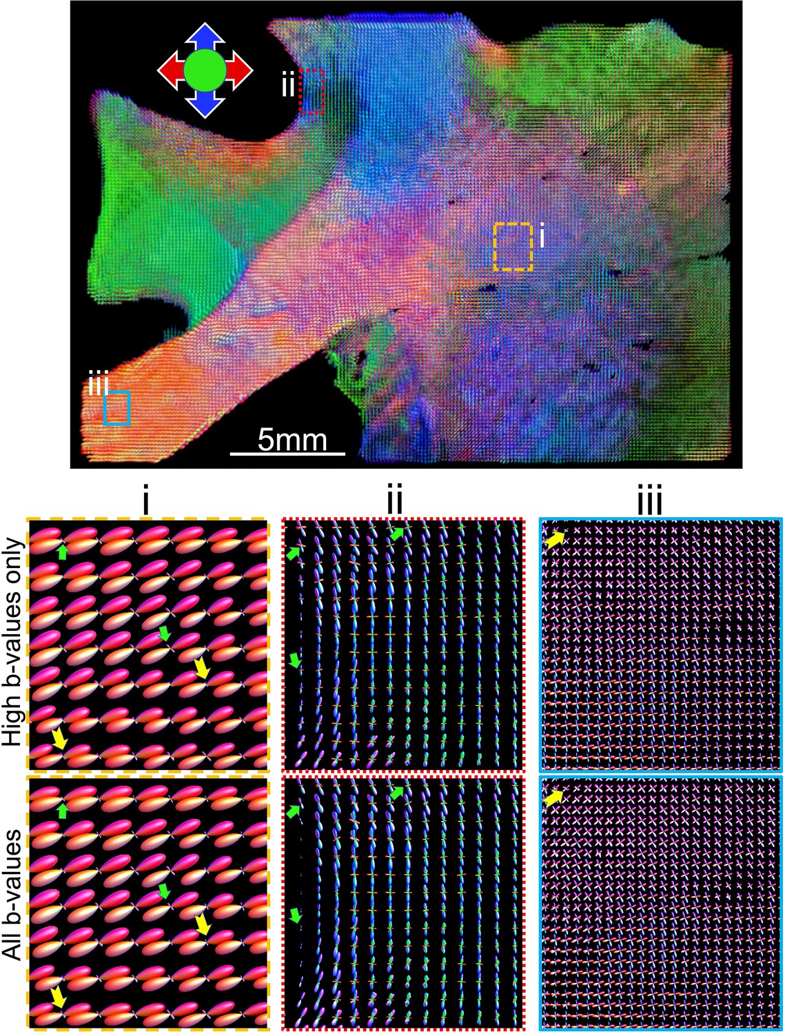
MRI fiber orientations of the posterior human brain section no. 18, calculated from all b-values and high b-values only (high b-values: 5 and 10 ms/μm2), with enlarged boxes i, ii, iii at the bottom.
Orientation distributions appear almost identical. Green flat-bottomed arrows indicate some of the few voxels where high b-values yield slightly stronger secondary orientations, and yellow arrow-bottomed arrows indicate some of the few voxels where all b-values yield slightly stronger secondary orientations,.
Figure 5—figure supplement 5
Single and crossing small-angle X-ray scattering (SAXS)- and diffusion magnetic resonance imaging (dMRI)-derived fiber orientations per voxel for the posterior human brain section no. 18.
Figure 6
Pixel-wise comparison of 3D-scanning SAXS (3D-sSAXS)/diffusion magnetic resonance imaging (dMRI) fiber inclinations and scattered light imaging (SLI) peak distances.
The images on the left show the analysis of one vervet brain section (no. 511, Figure 2B); the images on the right show the analysis for one human brain section (posterior section, cf. blue rectangle in Figure 5B). 3D-sSAXS and dMRI images were registered onto the corresponding SLI images with 3 µm resolution (Figure 4—figure supplement 1); the fornix in the vervet brain section was additionally shifted between the SLI and 3D-sSAXS images to account for the slight misalignment between the registered images in this region; only regions with unidirectional fibers were evaluated. (A,B) 3D-sSAXS fiber inclination angles of the vervet and human brain section are shown in different colors for the white matter (blue: in-plane, yellow: out-of-plane, dark gray: gray matter). The 3D-arrows indicate in four selected regions of the vervet brain section the orientation in which the fibers of these regions point out of the section plane. (C) Corresponding dMRI fiber inclination angles of the human brain sample. (D,E) Distance between two peaks in the corresponding SLI azimuthal profiles (cf. inset in G). Only profiles with one or two azimuthal peaks were evaluated (other pixels are shown in light gray). Regions used for the pixel-wise comparison with 3D-sSAXS are surrounded by colored outlines; asterisks mark three representative pixels. (F) dMRI orientation distribution functions of the region marked in C. The dashed lines indicate separation into the three regions in E (cg – cingulum, CiG – cingulate gyrus, cc - callosum). (G) SLI peak distance plotted against the 3D-sSAXS inclination for the corresponding regions marked in D and E for vervet and human brain samples, respectively (data points are displayed in similar colors as the corresponding outlines in D and E). The inset in the left panel shows the SLI azimuthal profiles for the three representative pixels in the vervet brain section (marked by similarly colored asterisks in D and G). The SLI profiles were centered for better comparison; the ticks on the inset x-axis denote azimuth steps of 15°. The dashed curves indicate the predicted SLI peak distance obtained from simulated scattering patterns of fiber bundles with different inclinations (Menzel et al., 2021a, Figure 7d).
Additional files
Download links
A two-part list of links to download the article, or parts of the article, in various formats.
Downloads (link to download the article as PDF)
Open citations (links to open the citations from this article in various online reference manager services)
Cite this article (links to download the citations from this article in formats compatible with various reference manager tools)
Using light and X-ray scattering to untangle complex neuronal orientations and validate diffusion MRI
eLife 12:e84024.
https://doi.org/10.7554/eLife.84024


