Cortical magnification eliminates differences in contrast sensitivity across but not around the visual field
- Department of Psychology, New York University, United States
- Center for Neural Science, New York University, United States
Figures
Figure 1
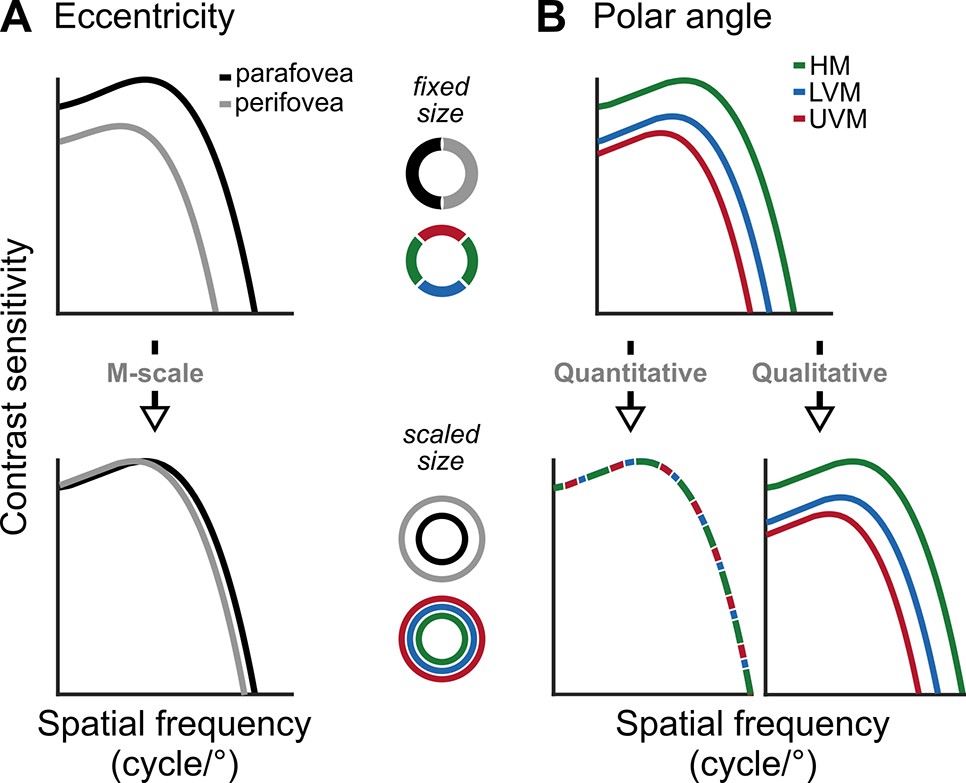
Schematic predictions of contrast sensitivity functions (CSFs).
(A) CSFs decline between the parafovea (2°) and perifovea (6°) for fixed-sized gratings (top row), but differences at low and medium SFs diminish after M-scaling Virsu and Rovamo, 1979 (bottom row). (B) CSFs differ among the horizontal meridian (HM), lower vertical meridian (LVM), and upper vertical meridian (UVM) for fixed-sized stimuli (top row). If polar angle asymmetries derive from differences in neural count among locations, M-scaling will diminish them (‘quantitative’ hypothesis). Alternatively, if the asymmetries derive from qualitatively different neural image-processing capabilities among locations, then M-scaling will not eliminate them (‘qualitative’ hypothesis).
Figure 2
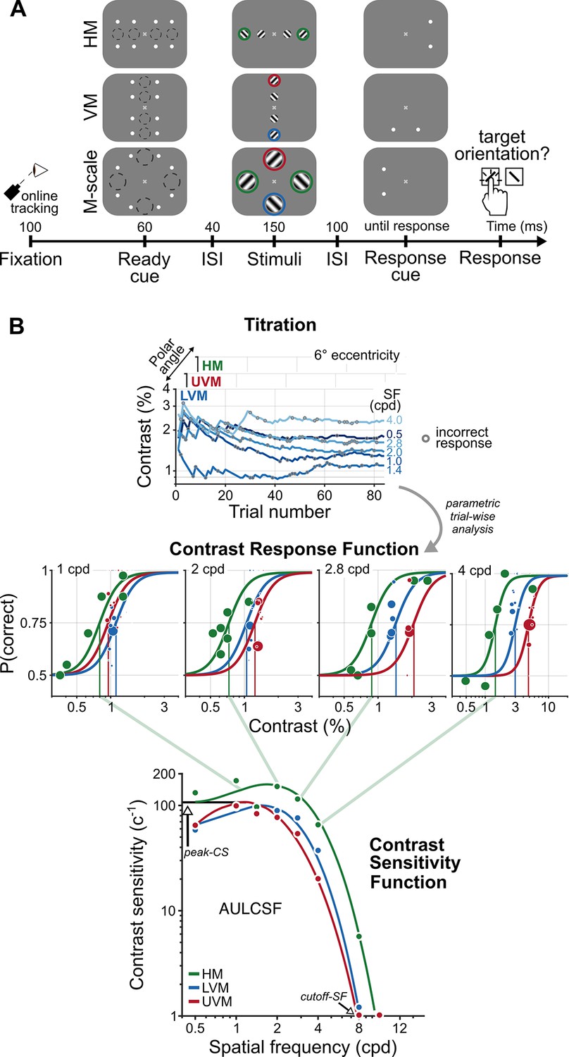
A psychophysical procedure to measure and a parametric model to characterize contrast sensitivity functions (CSFs).
(A) An example trial sequence for the orientation discrimination task. Each trial began with a fixation period, after which a cue indicated the onset of four gratings. The dashed circles illustrate the location and size of the grating stimuli; they did not appear during the experiment. Gratings appeared in the parafovea (2° eccentricity) and perifovea (6° eccentricity), separately along the horizontal (HM) or vertical meridian (VM) or were M-scaled, and presented simultaneously at each meridional location in the perifovea (M-scale). A response cue indicated which grating observers should report. The colored circles indicate the perifoveal locations we compared to assess the impact of M-scaling on polar angle asymmetries: Green, HM; blue, lower VM (LVM); red, upper VM (UVM). (B) Parametric contrast sensitivity model. Grating contrast varied throughout the experiment following independent titration procedures for each eccentricity and polar angle location. Gray circles indicate incorrect responses for a given trial (top row). A model composed of contrast response functions (CRF, middle row) and CSFs (bottom row) constrained the relation between trial-wise performance, SF, eccentricity, and polar angle. The diagonal green lines depict the connection between contrast thresholds from individual CRFs to contrast sensitivity on the CSF for the HM; contrast sensitivity is the inverse of contrast threshold. The colored dots in each CRF and CSF depict a representative observer’s task performance and contrast sensitivity, determined directly from the titration procedures. The colored lines depict the best-fitting model estimates. We derived key attributes of the CSF – peak contrast sensitivity (peak-CS), the acuity limit (cutoff-SF), and the area under the log contrast sensitivity function (AULCSF) – from the fitted parametric model.
Figure 3
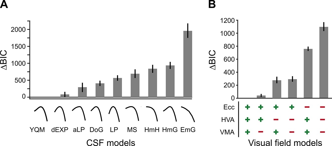
BIC model comparisons for contrast sensitivity function (CSF) and visual field models.
(A) CSF model comparisons for the nine candidate functional forms of the CSF applied to the group data (Table 1). Low ΔBIC values indicate superior model performance. Curves under each bar illustrate the best fit of each CSF model to a representative observer (n=10). (B) Visual field model comparisons (Table 2). ‘+’ and ‘-’ under each bar indicate the components included and excluded, respectively, in each model. For example, ‘+’ for ‘HVA’ indicates that CSFs could change between the horizontal and vertical meridians, whereas a ‘-’ indicates that CSFs for the horizontal meridian were identical to the lower vertical meridian.
Figure 4 with 1 supplement
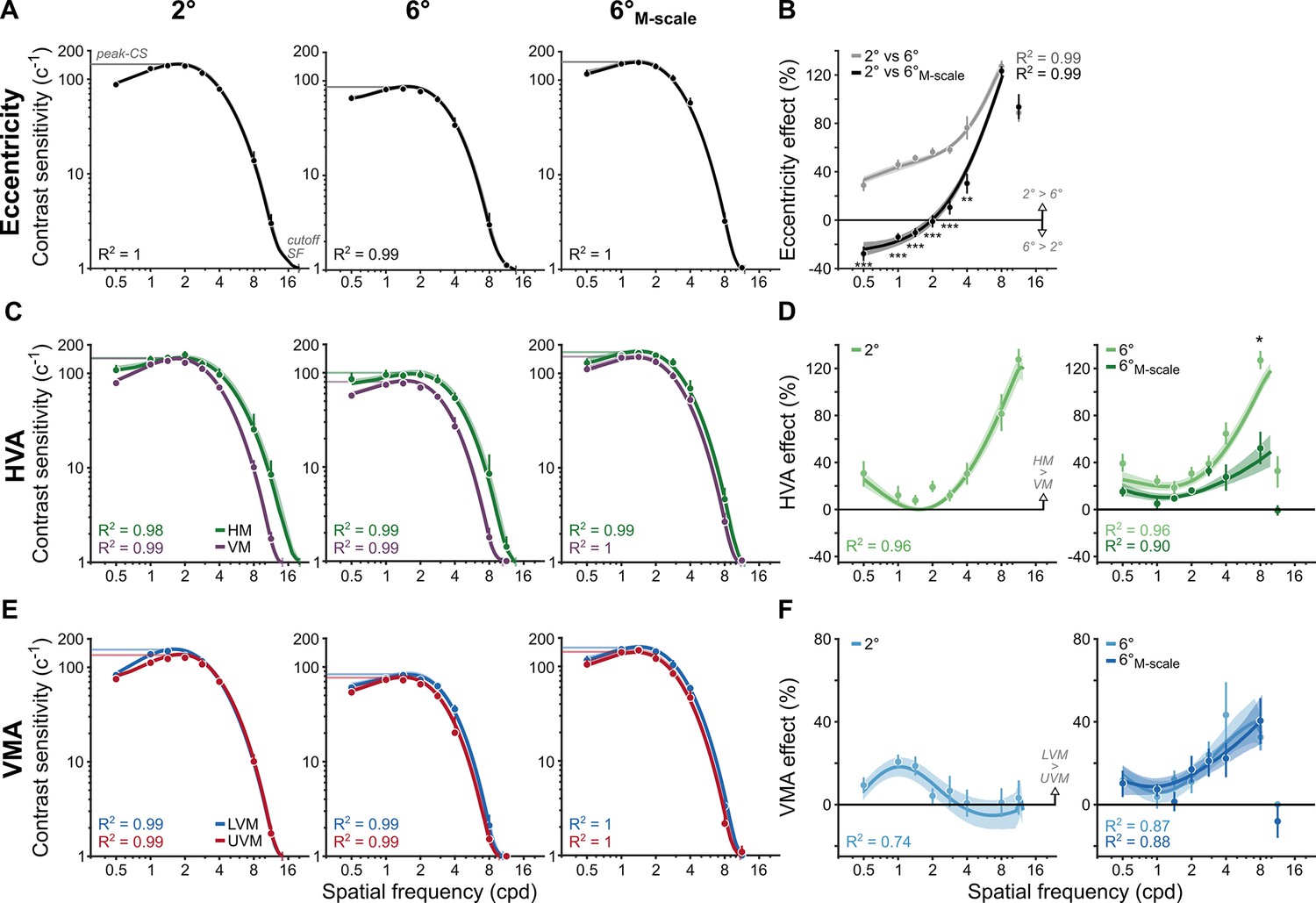
M-scaling diminishes the eccentricity effect, but neither the horizontal-vertical anisotropy (HVA) nor the vertical meridian asymmetry (VMA) (n=10).
(A) Contrast sensitivity functions (CSFs) averaged across polar angles for fixed-size gratings at 2° and 6°, as well as for M-scaled gratings at 6°. (B) Eccentricity effects are quantified as the percent change in contrast sensitivity between 2°and 6° as well as between 2° and 6°M-scale. Positive values indicate higher contrast sensitivity at 2° than 6°. Negative values indicate a reversal: higher contrast sensitivity at 6° than 2°. (C) CSFs for the horizontal meridian (HM) compared to the average CSF across the lower vertical meridian (LVM) and upper vertical meridian (UVM). (D) The percent change between horizontal and vertical meridians at 2° (left) and the percentage change between meridians for 6° and 6°M-scale (right). Values above 0% indicate higher sensitivity for the HM than VM. (E) CSFs for the LVM and UVM. (F) The percent change between LVM and UVM following the conventions in (D) (with a truncated y-axis); positive values indicate higher sensitivity for the LVM than UVM. All dots correspond to the group-average (n=10) contrast sensitivity and percent change in contrast sensitivity, as estimated from the titration procedures. Lines in panels (A, C, E) correspond to the group-average fit of the parametric contrast sensitivity model. Lines in panels (B, D, F) correspond to group average location percent differences as calculated in Equation 9 (see ‘Methods’). Note that the line does not reach the highest SF in these panels for the 6° and 6°M-scale comparison, as observers performed at chance, consistent with the fact that SF is harder to discriminate in the periphery. Error bars and shaded areas denote bootstrapped 68% confidence intervals. Repeated-measures ANOVA; *p<0.05, **p<0.01, ***p<0.001.
Figure 4—figure supplement 1
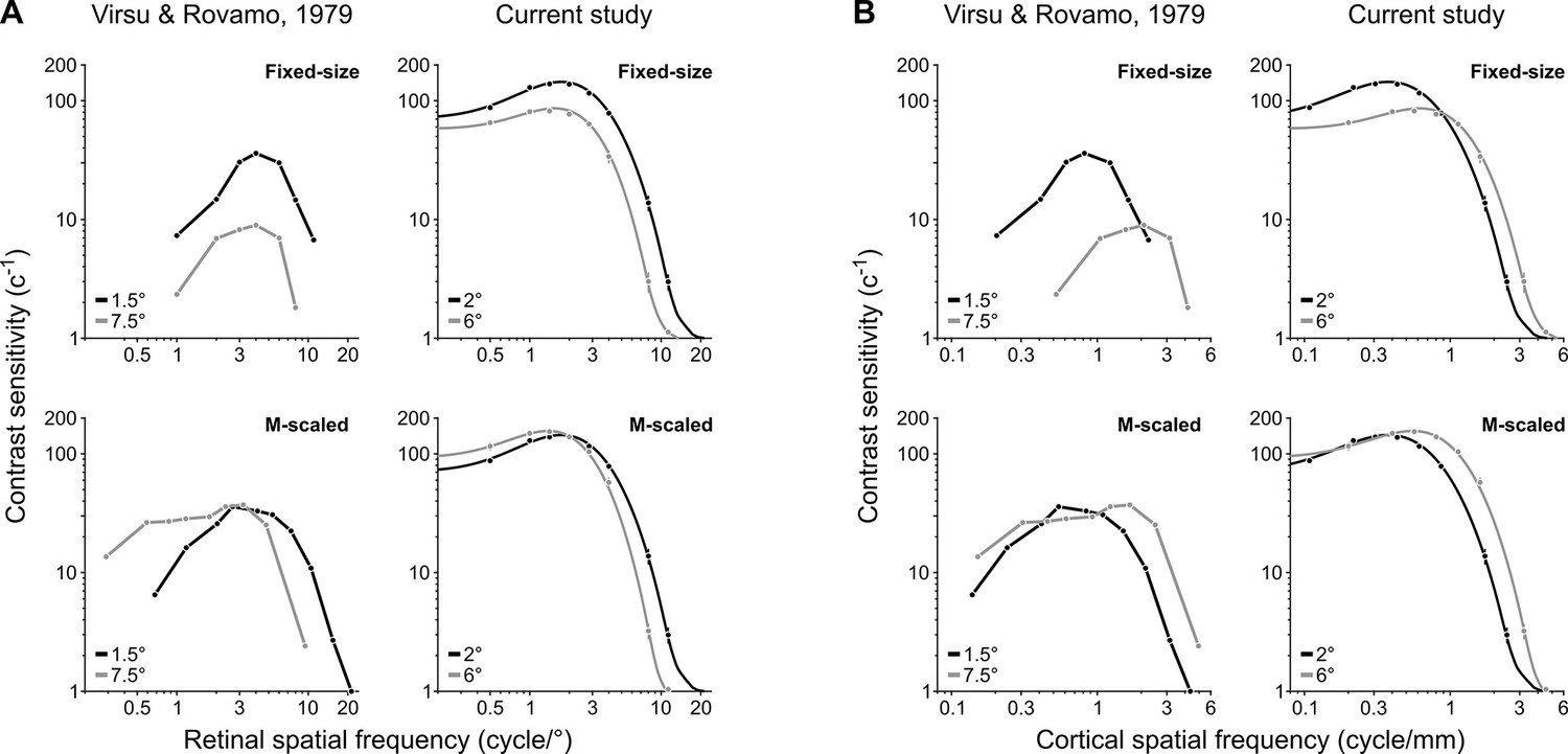
Qualitatively similar contrast sensitivity functions (CSFs) between previous reports (Rovamo and Virsu, 1979) and this study for fixed-size and M-scaled grating stimuli.
(A) CSFs expressed as a function of retinal spatial frequency (SF). For fixed-size stimuli, CSFs decline with increasing eccentricity at all SFs. After M-scaling, contrast sensitivity for the farther eccentricity exceeds that of the nearer eccentricity at low SFs. (B) CSFs expressed as a function of cortical SF. We used equations in Virsu and Rovamo, 1979 to determine the SF when projected onto the cortical surface at each eccentricity, resulting in the cycles per millimeter of striate-cortical surface area. The data for Virsu and Rovamo, 1979 depict contrast sensitivity for an individual observer as plotted in Figure 4 of Virsu and Rovamo, 1979. We extracted only the eccentricities most comparable to those tested in this study. The CSFs displayed under ‘current study’ follow the conventions of Figure 4.
Figure 5 with 1 supplement

Polar angle asymmetries emerge in key contrast sensitivity function (CSF) attributes.
(A, B) Peak contrast sensitivity for the horizontal-vertical anisotropy (HVA) and vertical meridian asymmetry (VMA), respectively. (C, D) Cutoff-SF for the HVA and VMA, respectively. (E, F) Area under the log contrast sensitivity function (AULCSF) for the HVA and VMA, respectively. Each bar depicts the group-average (n=10) attribute at a given location, and error bars depict bootstrapped 68% confidence intervals. Horizontal gray lines denote significant comparisons of an ANOVA and of post hoc comparisons. The vertical lines displayed on the gray bars depict the 68% confidence interval for the differences between eccentricities or locations. Repeated-measures ANOVA; *p<0.05, **p<0.01, ***p<0.001.
Figure 5—figure supplement 1
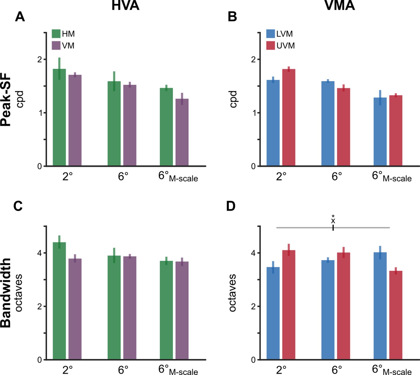
Neither polar angle asymmetries nor eccentricity effects emerge in retinal peak spatial frequency (SF) and SF bandwidth.
(A, B) Peak SF for the horizontal-vertical anisotropy (HVA) and vertical meridian asymmetry (VMA), respectively. (C, D) SF bandwidth for the HVA and VMA, respectively. Each bar depicts the group-average (n=10) attribute at a given meridional location. and error bars depict 68% confidence intervals. A significant interaction emerged in the bandwidth for the VMA (F(2,18) = 5.21, p=0.019, ηG2 = 0.367). However, none of the post hoc comparisons reached significance (all p>0.1). No other statistical comparisons were significant.
Figure 6
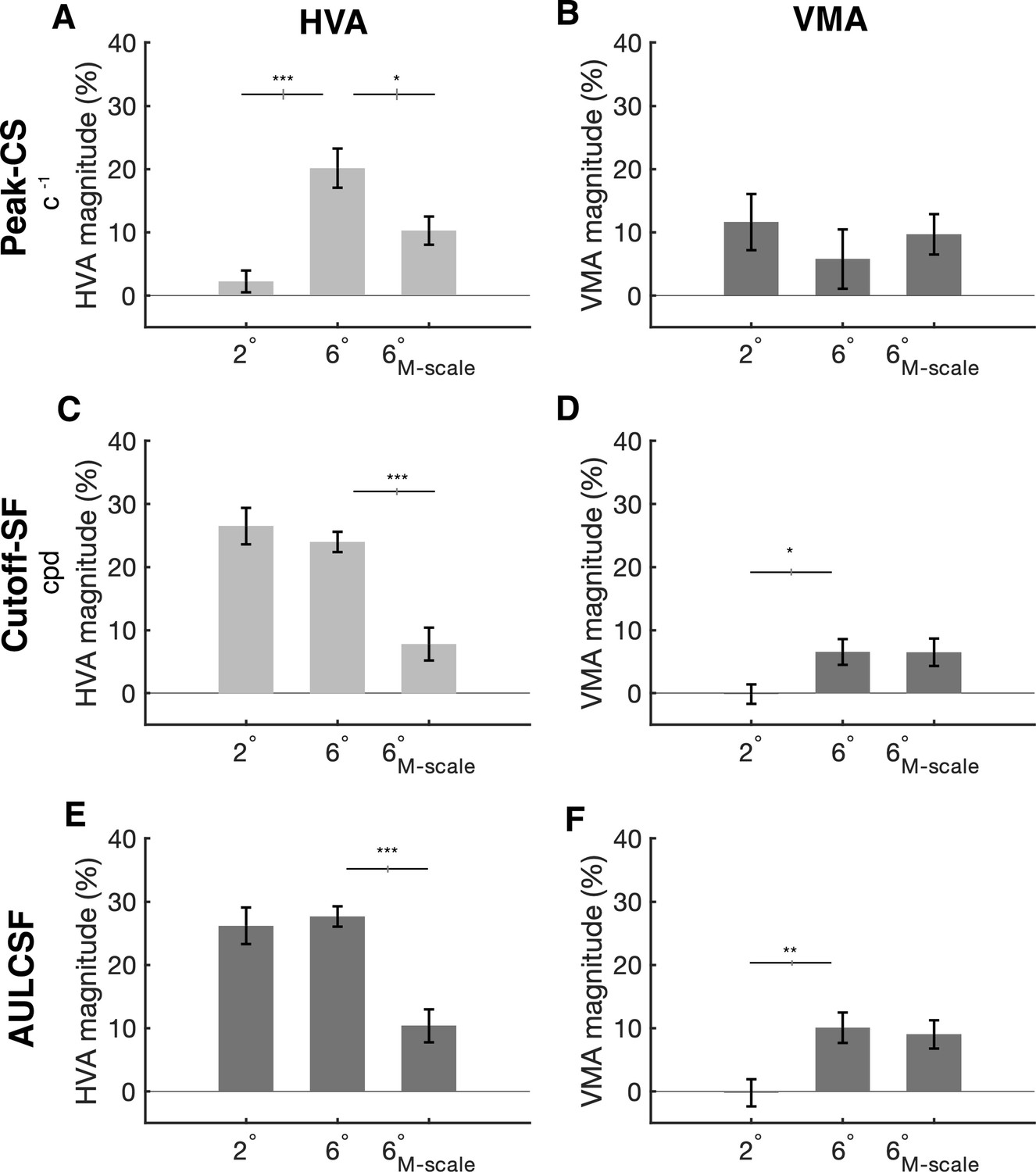
Horizontal-vertical anisotropy (HVA) and vertical meridian asymmetry (VMA) magnitudes for peak contrast sensitivity, spatial frequency cutoff, and area under the log contrast sensitivity function curve (AULCSF).
(A, B) Peak contrast sensitivity for the HVA and VMA, respectively, at 2°, 6°, and 6°M-scale. (C, D) Cutoff-SF for the HVA and VMA, respectively, at 2°, 6°, and 6°M-scale. (E, F) AULCSF for the HVA and VMA, respectively, at 2°, 6°, and 6° M-scaled. n=10. Error bars representing ±1 standard error of the mean (SEM) and horizontal gray lines denote significant comparisons of an ANOVA and post hoc comparisons. Vertical lines displayed on the gray bars denote the standard error of the difference (SED). *p<0.05, **p<0.01, ***p<0.001.
Figure 7
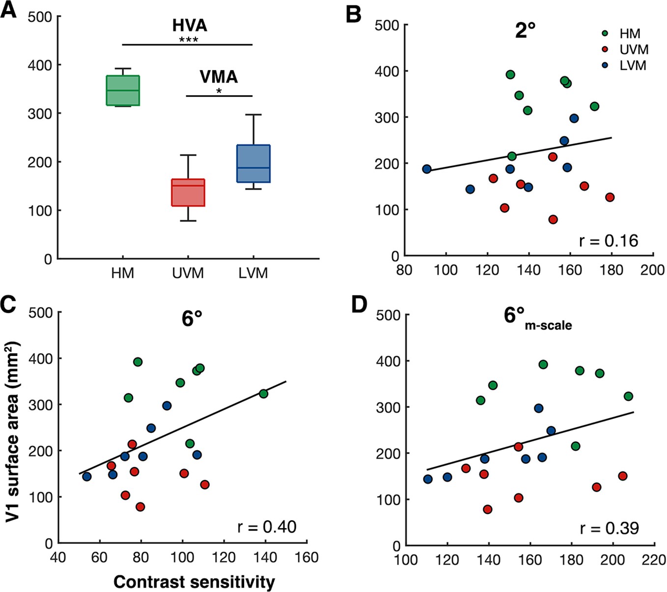
Individualized V1 surface area measurements at the cardinal meridians correlate with peak contrast sensitivity measurements.
(A) Group-level V1 surface area measurements (n=7) taken from the cortical representation of the horizontal meridian (HM) (mean of left and right HM), the upper vertical meridian (UVM), and lower vertical meridian (LVM). *p<0.05, ***p<0.001. (B–, C) Between-subject Spearman’s correlations of V1 surface area (±15° of angle, 1–8° eccentricity) at each meridian with peak contrast sensitivity measurements (n = 7, 3 measurements per observer) at the same meridian for (B) 2°, (C) 6°, and (D) 6°-M-scale stimulus conditions.
Tables
Table 1
Candidate contrast sensitivity function (CSF) models.
The number of parameters included in each model (n) is denoted under the corresponding label, along with a brief description and the model equation. The bolded entry indicates the best-fitting model.
| Label (n) | Description | Equation |
|---|---|---|
| YQM (4) | Derived from a model of contrast sensitivity Chung and Legge, 2016 | |
| dEXP (3) | Double exponential function Chakravarthi et al., 2022 | |
| aLP (4) | Asymmetric log parabola Corbett and Carrasco, 2011 | |
| DoG (4) | Difference of Gaussians Chung and Legge, 2016 | |
| LP (3) | Log parabola Chung and Legge, 2016 | |
| MS (4) | Generalized Gaussian with linear function of SF Chung and Legge, 2016 | |
| HmH (4) | Difference of hyperbolic secants Chung and Legge, 2016 | |
| HmG (4) | Hyperbolic secant minus a Gaussian Chung and Legge, 2016 | |
| EmG (4) | Exponential minus a Gaussian Chung and Legge, 2016 |
Table 2
Models of contrast sensitivity across eccentricity and polar angle.
The bolded entry indicates the best-fitting model.
| Model label | Description | Max number of parameters |
|---|---|---|
| Ecc + HVA + VMA | CSFs vary across eccentricity and polar angle | 24 |
| Ecc +HVA - VMA | CSFs do not vary along the VM | 16 |
| Ecc - HVA + VMA | CSFs do not vary along the HM | 16 |
| -Ecc + HVA + VMA | CSFs do not vary across eccentricity | 12 |
| Ecc - HVA - VMA | CSFs do not vary along the VM and HM | 8 |
| -Ecc - HVA - VMA | CSFs are identical at all visual field locations | 4 |
-
CSF: contrast sensitivity function; VM: vertical meridian; HM: horizontal meridian; HVA: horizontal-vertical anisotropy; VMA: vertical meridian asymmetry.
Additional files
Download links
A two-part list of links to download the article, or parts of the article, in various formats.
Downloads (link to download the article as PDF)
Open citations (links to open the citations from this article in various online reference manager services)
Cite this article (links to download the citations from this article in formats compatible with various reference manager tools)
Cortical magnification eliminates differences in contrast sensitivity across but not around the visual field
eLife 12:e84205.
https://doi.org/10.7554/eLife.84205


