Figures and data in Dynamics of co-substrate pools can constrain and regulate metabolic fluxes

Figures
Tables
Additional files

18 figures, 2 tables and 2 additional files

Figures

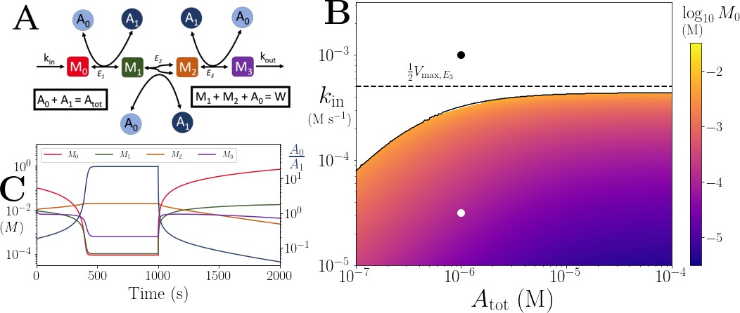
Figure 1

Download asset Open asset

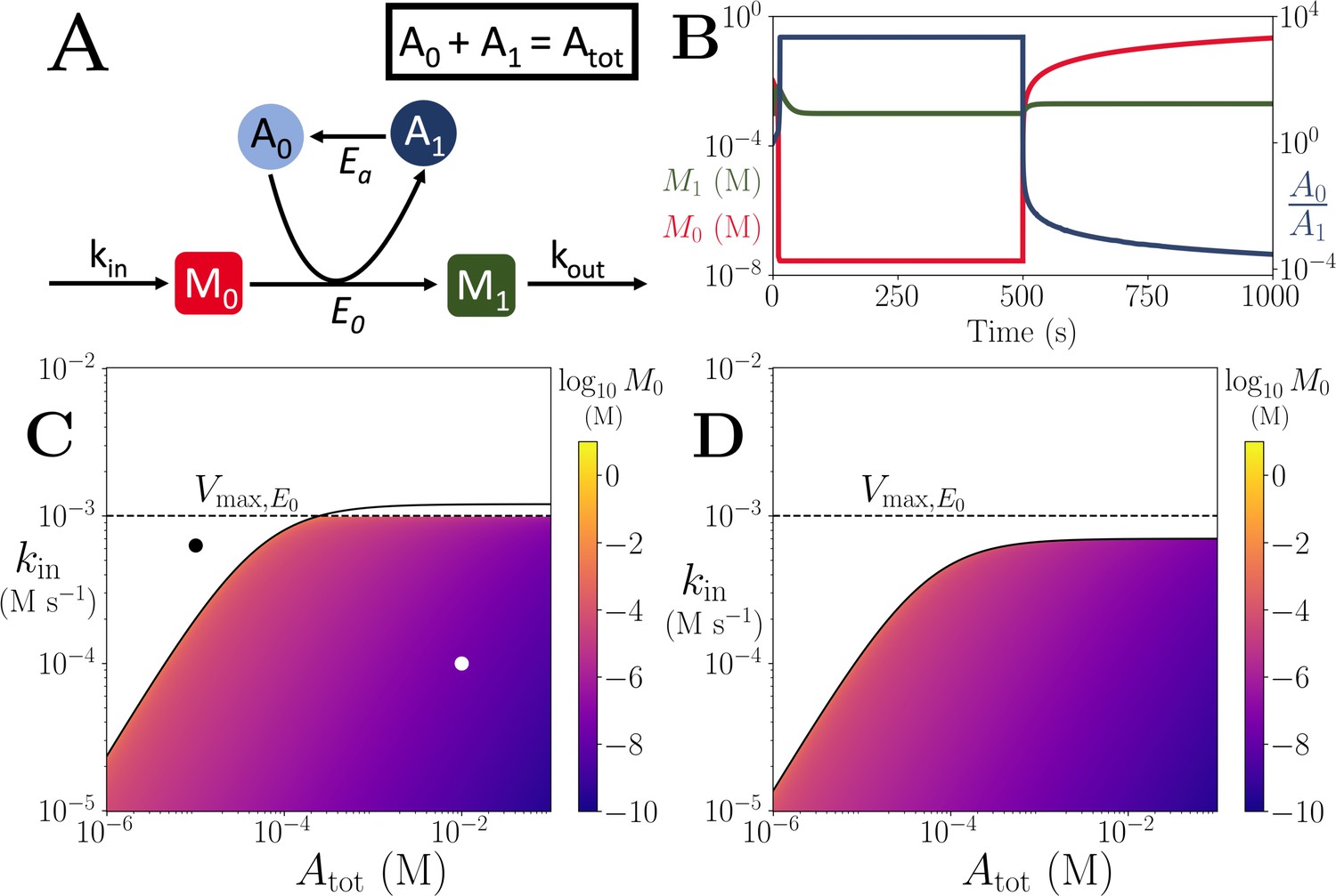
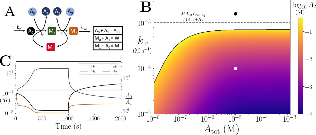
Motif, time-series and threshold in a single co-substrate involving reaction.

(A) Cartoon representation of a single irreversible reaction with co-substrate cycling (see Appendices for other reaction schemes). The co-substrate is considered to have two forms A₀ and A₁. (B) Concentrations of the metabolites M₀ (red) and M₁ (green), and the $A_{0} / A_{1}$ ratio (blue) are shown as a function of time. At $t = 500$ , the parameters are switched from the white dot in panel (C) (where a steady state exists) to the black dot (where we see continual build-up of M₀ and decline of A₀ without steady state). (C & D) Heatmap of the steady state concentration of M₀ as a function of the total co-substrate pool size ( $A_{tot}$ ) and inflow flux (k_in). White area shows the region where there is no steady state. On both panels, the dashed line indicates the limitation from the primary enzyme, $k_{i n} < V_{m a x, E_{0}}$ , and the solid line indicates the limitation from co-substrate cycling, $k_{i n} < A_{t o t} V_{m a x, E_{a}} / (K_{M, E_{a}} + A_{t o t})$ . In panel (C), there is a range of $A_{tot}$ values for which the first limitation is more severe than the second. In contrast, in panel (D), the second limitation is always more severe than the first. In (B & C) the parameters used for the primary enzyme (for the reaction converting M₀ into M₁) are picked from within a physiological range (see Supplementary file 1) and are set to: $E_{tot} = 0.01$ mM, $k_{c a t} = 100 / s$ , $K_{M, E_{0}} = K_{M, E_{a}} = 50 μ M$ , while k_out is set to 0.1/s. The $E_{tot}$ and k_cat for the co-substrate cycling enzyme are 1.2 times those for the primary enzyme. In panel (D) the parameters are the same except for the $E_{tot}$ and k_cat of the co-substrate cycling enzyme, which are set to 0.7 times those for the primary enzyme.

Figure 2

Download asset Open asset

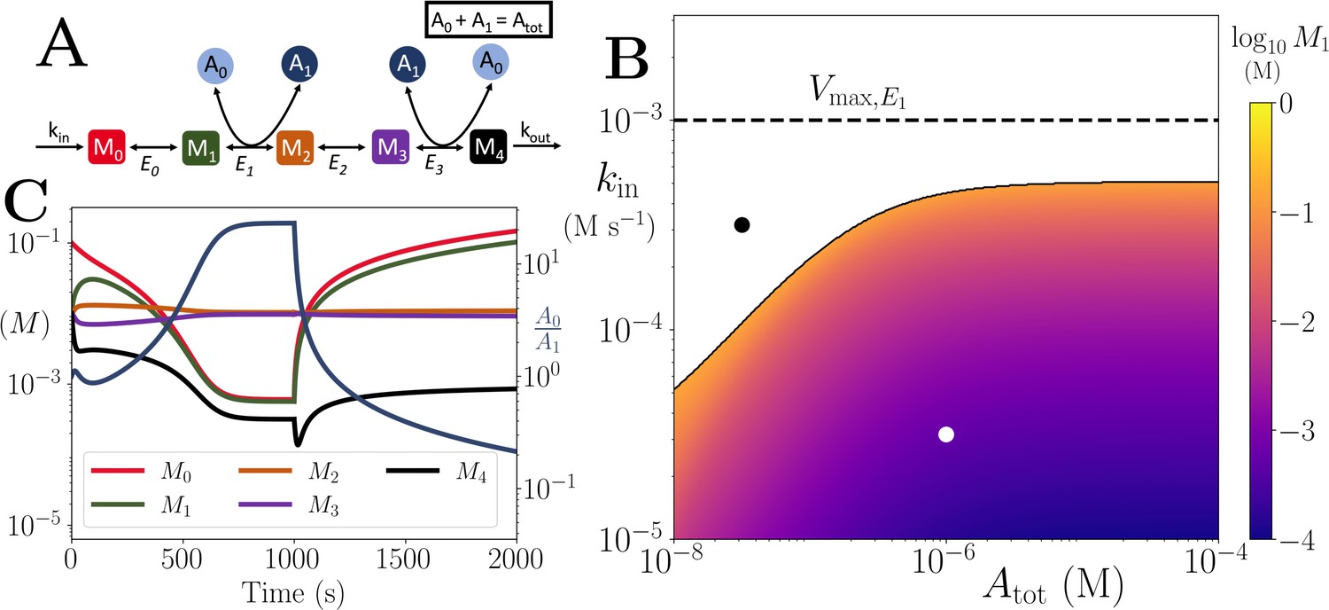
Motif, time-series and thresholds for the linear pathway model with $n = 4$ .

(A) Cartoon representation of a chain of reversible reactions with co-substrate cycling occurring solely inter-pathway. The co-substrate is considered to have two forms A₀ and A₁. (B) Heatmap of the steady state concentration of M₀ as a function of the total metabolite pool size ( $A_{tot}$ ) and inflow rate constant (k_in). White area shows the region where there is no steady state. The dashed and solid lines indicate the limitations arising from primary enzyme (E₁ in this case) and co-substrate cycling, respectively, as in Figure 1. (C) Concentrations of $M_{0 - 4}$ , and $A_{0} / A_{1}$ ratio as a function of time (with colours as indicated in the inset). At $t = 1000$ s, the parameters are switched from the white dot in panel (B) (where a steady state exists) to the black dot (where we see build-up of all substrates that are produced before the first co-substrate cycling reaction, and continued decline of A₀). The parameters used are picked from within a physiological range (see Supplementary file 1) and are set to: $E_{tot} = 0.01$ mM, $k_{c a t} = 100 / s$ , $K_{M} = 50 μ m$ , for all reactions, and $k_{o u t} = 0.1 / s$ .

Figure 3

Download asset Open asset

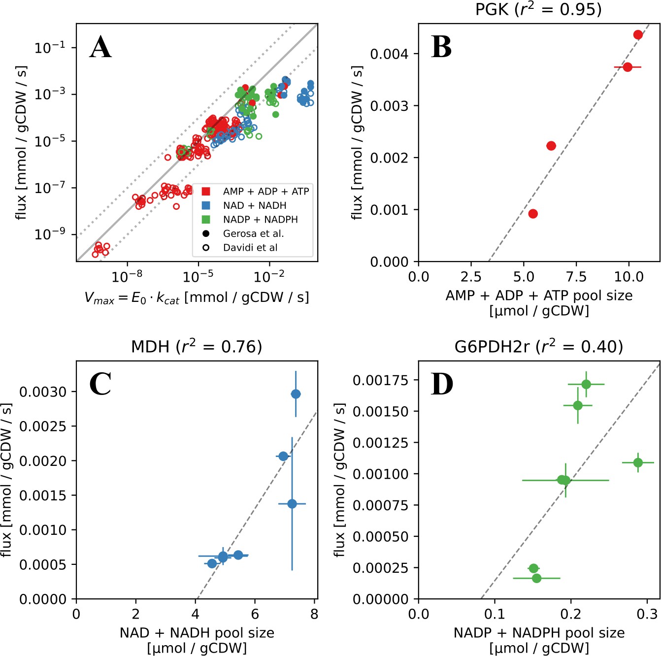
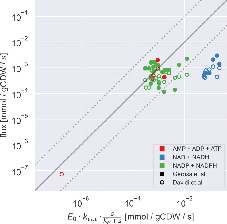
Measured and FBA-predicted flux values are typically lower than the calculated primary enzyme threshold.

(A) Measured and FBA-predicted flux values (from Davidi et al., 2016; Gerosa et al., 2015) plotted against the calculated primary enzyme kinetic threshold (first part of eq. (1)). Notice that there are 7 points for each reaction, corresponding to the different experimental conditions under which measurements or FBA modelling was done (see Supplementary file 1 for data, along with reaction names and metabolites involved). (**B–D**) Measured flux values under different experimental conditions (from Gerosa et al., 2015) for select reactions plotted against the corresponding co-substrate pool size. Panels B to D show reactions for phosphoglycerate kinase (*PGK*), malate dehydrogenase (*MDH*), and glucose-6-phosphate dehydrogenase (*G6PDH*). Each point on these panels is a separate flux measurement under a different environmental condition, where the co-substrate pool size is also measured. Error bars represent standard deviations of flux and metabolite measurements as they appear in the dataset from Gerosa et al. Point colours represent co-substrate type and are as shown in the legend to panel A. Lines show the best linear fit with the corresponding normalised RMSE shown in the panel title.

Figure 4

Download asset Open asset

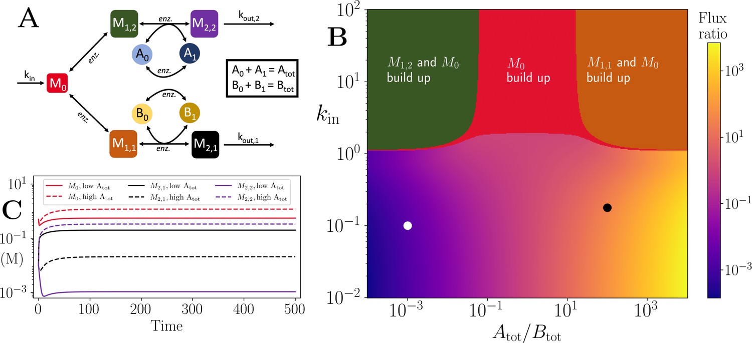
Motif, heatmap and time-series for the branching pathway model.

(A) Cartoon representation of two branching pathways from the same upstream metabolite. The two branches are linked to separate co-substrate pools, $A$ and $B$ . Note that pathway independent turnover of the co-substrates is included in the model (see Figure 4—source code 1). (B) The pathways’ flux ratio (i.e. flux into $M_{2, 2}$ divided by flux into $M_{2, 1}$ ) shown in colour mapping, against the ratio of co-substrate pool sizes, $A_{tot}$ and $B_{tot}$ , and the influx rate, k_in, into the upstream metabolite. In the block colour areas, the system has no steady state and the indicated metabolite(s) M₀ and one of the metabolites $M_{1, 2}$ or $M_{1, 1}$ accumulate towards infinity. (C) Concentrations of upstream and branch-endpoint metabolites over time, coloured as shown in the inset of the panel. The solid lines show results using parameters indicated by the white dot in panel (B), where $B_{t o t} > A_{t o t}$ , while the dashed lines show results using parameters indicated by the black dot in panel (B), where $A_{t o t} > B_{t o t}$ . For both simulations, all kinetic parameters are arbitrarily set to 1, apart from the pathway-independent co-substrate recycling ( $V_{\max, E_{a}}$ and $V_{\max, E_{b}}$ ) that is set to 10 (see Figure 4—source code 1).

Figure 4—source code 1 Python implementation of branched pathway model, presented in Figure 4.: https://cdn.elifesciences.org/articles/84379/elife-84379-fig4-code1-v2.zip
Download elife-84379-fig4-code1-v2.zip

Figure 5

Download asset Open asset

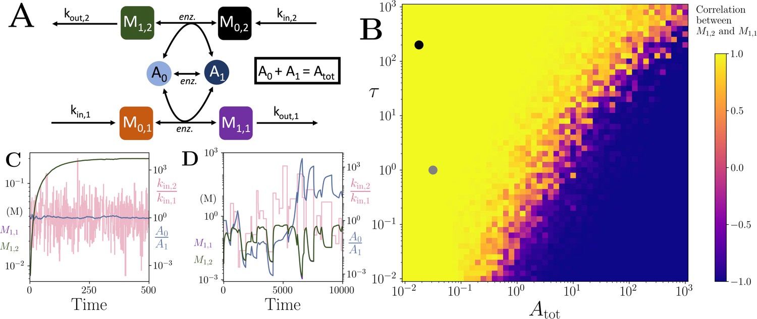
Motif, heatmap and time-series for the coupled pathway model with noisy influxes.

(A) Cartoon representation of two pathways coupled via the same co-substrate cycling. The two forms of the co-substrate are indicated as A₀ and A₁. It is converted from A₀ to A₁ on the lower pathway, and from A₁ to A₀ in the upper pathway. The presented results are for a model with reversible enzyme kinetics, while the results from a model with irreversible enzyme kinetics are shown in Appendix 10—figure 2. (B) Correlation coefficient of the two pathway product metabolites, $M_{1, 2}$ and $M_{1, 1}$ , as a function of the total amount of co-substrate ( $A_{tot}$ ) and the extent of fluctuations in the two pathway influxes, $k_{in, 1}$ and $k_{in, 2}$ . The influx fluctuation is characterised by a waiting time that is exponentially distributed with mean $τ$ , after which the log ratio of the k_in values is drawn from a standard normal distribution. The mean of the k_in values is set to be 0.1 and the pathway-independent cycling occurs at a much lower rate compared to the other reactions (see Figure 5—source code 1). (C) Concentrations of metabolites $M_{1, 2}$ (green) and $M_{1, 1}$ (magenta), pathway influx ratio (pink), and $A_{0} / A_{1}$ ratio (blue) as a function of time. The simulation is run with parameters corresponding to the grey dot in (B) where the products are correlated, and the rate of k_in fluctuations is on a similar timescale to the other reactions. The system is largely unresponsive to the noise, and the $M_{1, 2}$ and $M_{1, 1}$ are fully correlated (i.e. the green and magenta curves overlap). (D) Concentrations of metabolites $M_{1, 2}$ (green) and $M_{1, 1}$ (magenta), pathway influx ratio (pink), and $A_{0} / A_{1}$ ratio (blue) as a function of time. The simulation is run with parameters corresponding to the black dot in (B) where the products are correlated, but the fluctuations in k_in values occur at a much lower rate than the other reactions. The system is responsive to the noise, yet the $M_{1, 2}$ and $M_{1, 1}$ are fully correlated (i.e. the green and magenta curves overlap). For both simulations, all kinetic parameters are arbitrarily set to 1, apart from the pathway-independent co-substrate recycling ( $V_{\max, E_{a}}$ ) that is set to 0.01 (see Figure 5—source code 1).

Figure 5—source code 1 Python implementation of connected pathway model, presented in Figure 5.: https://cdn.elifesciences.org/articles/84379/elife-84379-fig5-code1-v2.zip
Download elife-84379-fig5-code1-v2.zip

Appendix 1—figure 1

Download asset Open asset

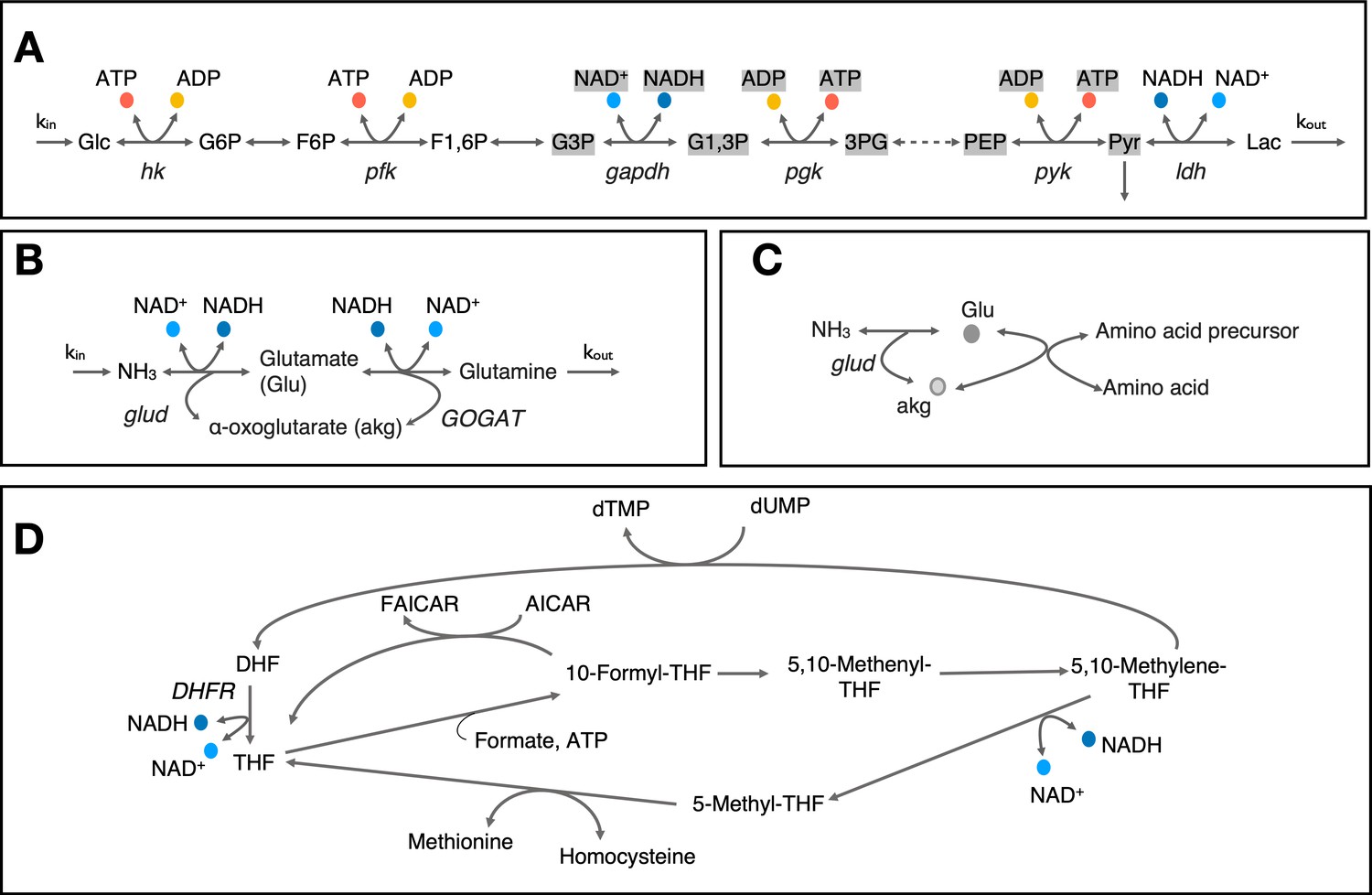
Cartoon representation of select metabolic pathways involving co-substrate cycling.

(A) Cartoon representation of upper glycolysis pathway. Note that stoichiometric balance across the pathway changes after F1,6P and metabolites and co-substrates highlighted with gray background have a stoichiometry of 2. (**B & C**) Cartoon representation of nitrogen assimilation via glutamate and involvement of glutamate cycling in amino acid biosynthesis. (D) Cartoon representation of metabolite cycles involved in one-carbon metabolism around tetrahydorfolate. Enzyme and metabolite name abbreviations are: Glc – Glucose, G6P – Glucose-6-phosphate, F6P – Fructose-6-phosphate, F1,6P – Fructose-1,6-biphosphate, G3P – glyceraldehyde-3-phosphate, G1,3P – 1,3-biphospho-D-glycerate, 3 PG – 3-phospho-D-glycerate, PEP – Phosphoenolpyruvate, Pyr – Pyruvate, Lac – Lactate, DHF – Dihydrofolate, THF - Tetrahydrofolate, AICAR - 5-amino-4-imidazolecarboxamide ribotide, FAICAR - 5’-phosphoribosyl-formamido-carboxamide, hk – hexokinase, pfk – phosphofructokinase, gapdh – glyceraldehyde-3-phosphate dehydrogenase, pgk – phosphoglycerate kinase, pyk – phophoenolpyruvate kinase, ldh – lactate dehydrogenase, glud – glutamate dehydrogenase, GOGAT – glutamate synthase, DHFR – dihydrofolate reducatase.

Appendix 3—figure 1

Download asset Open asset

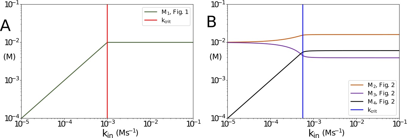
Concentrations of non-accumulating metabolites vs k_in in the models presented in Figures 1 and 2 of the main text.

(A) Concentration of non-accumulating metabolite M₁ from Figure 1. Red line shows the critical $k_{in}$ value, after which the concentration of M₁ remains constant (B) Concentrations of non-accumulating metabolites from the models presented in Figure 2. Blue line shows the threshold value for k_in. Once the threshold value for k_in is reached the concentrations of the non-accumulating metabolites do not change. $A_{tot} = 10^{- 1}$ in panel (A) and 10^-6 in panel (B). All other parameters are the same as their counterparts in the main text.

Appendix 5—figure 1

Download asset Open asset

Motif, time series and threshold for the linear pathway model with multiple co-substrates.

(A) Cartoon representation of a chain of reversible reactions with metabolite cycling of two different metabolites, as shown in Equation 33. Each cycled metabolite has two forms, and there is no pathway independent cycling. (B) Heatmap of of the steady state concentration of M₀ as a function of the metabolite pool sizes ( $A_{tot} = B_{tot}$ ) and the inflow flux (k_in). White area shows the region where there is no steady state. (C) Concentrations of $M_{0 - 4}$ , $A_{0} / A_{1}$ and $B_{0} / B_{1}$ ratios as a function of time. At $t = 1000$ s, parameters are switched from the white dot in panel (B) (where a steady state exists) to the black dot (where we see build up of M₀), and continued decline of A₀. The $B_{0} / B_{1}$ ratio remains constant however as these are still cycled by reactions after the build up. In (B) and (C) the other parameters are $k_{cat} = 100 s^{- 1}$ , $E_{tot} = 0.01 m M$ , $K_{m} = 50 μ M$ and $k_{out} = 0.1 s^{- 1}$ .

Appendix 6—figure 1

Download asset Open asset

Motif, time series and threshold for a model with differential co-substrate stoichiometry, as seen in glycolysis.

(A) Reaction system modelled in Appendix 6. Branching arrowhead from M₁ to M₂ indicates that two M₂ molecules are produced/used in the forward/backward reactions. (B) Heatmap of the steady state M₀ concentration. In the white area there is no steady state due to continual build up of M₀. Dashed line shows the smallest limit imposed by Equation 35. (C) Time series of $M_{0 \to 4}$ and $A_{0} / A_{1}$ . At $t = 1000$ s, parameters are switched from the white dot in panel (B) (where a steady state exists) to the black dot (where we see build up of M₀). Note that in the build up regime, M₂ reduces as well as $A_{0} / A_{1}$ , as M₂ production is dependent on the presence of A₀. In (B) and (C) the other parameters are $k_{cat} = 100 s^{- 1}$ , $E_{tot} = 0.01 m M$ , $K_{m} = 50 μ M$ and $k_{out} = 0.1 s^{- 1}$ .

Appendix 7—figure 1

Download asset Open asset

Motif, time series and threshold for model with both co-substrate and metabolite cycling, mimicking nitrogen assimilation.

(A) Reaction system modelled in Appendix 7. (B) Heatmap of the steady state A₂ concentration. In the white area there is no steady state due to continual build up of A₂. Dashed line shows the limit $k_{in} < \frac{M T E_{2}}{M T + K_{2}}$ , which is the smallest limit for these parameters. (C) Time series of $M_{0 \to 2}$ , A₂ and $A_{0} / A_{1}$ . At $t = 1000$ s, parameters are switched from the white dot in panel (B) (where a steady state exists) to the black dot (where there is continual build up of A₂). In (B) and (C) the other parameters are $k_{cat} = 100 s^{- 1}$ , $E_{tot} = 0.01 m M$ , $K_{m} = 50 μ M$ and $k_{out} = 0.1 s^{- 1}$ .

Appendix 8—figure 1

Download asset Open asset

Measured flux values (from Davidi et al., 2016; Gerosa et al., 2015) plotted against the calculated primary enzyme kinetic threshold (first part of Eq. (1) of the main text) adjusted by substrate affinity of the enzyme.

Note that the flux data shown here is a subset of the flux data presented in (Figure 3 of the main text), focusing only on those where the main substrate concentration was experimentally measured and the relevant $K_{M}$ is known. For both panels, the solid line indicates the equivalence of the two values and the dashed lines indicate 10-fold change interval on this, as a guide to the eye. Point colour indicates the nature of co-substrate involved and fill state indicates the data source (as shown on the inset).

Appendix 8—figure 2

Download asset Open asset

Cumulative distribution of the ratio of observed flux (measured or FBA-predicted) to enzyme kinetic based limit ( $V_{\max}$ ) (left panel) or to enzyme kinetic based limit accounting for substrate affinity (right panel).

Appendix 8—figure 3

Download asset Open asset

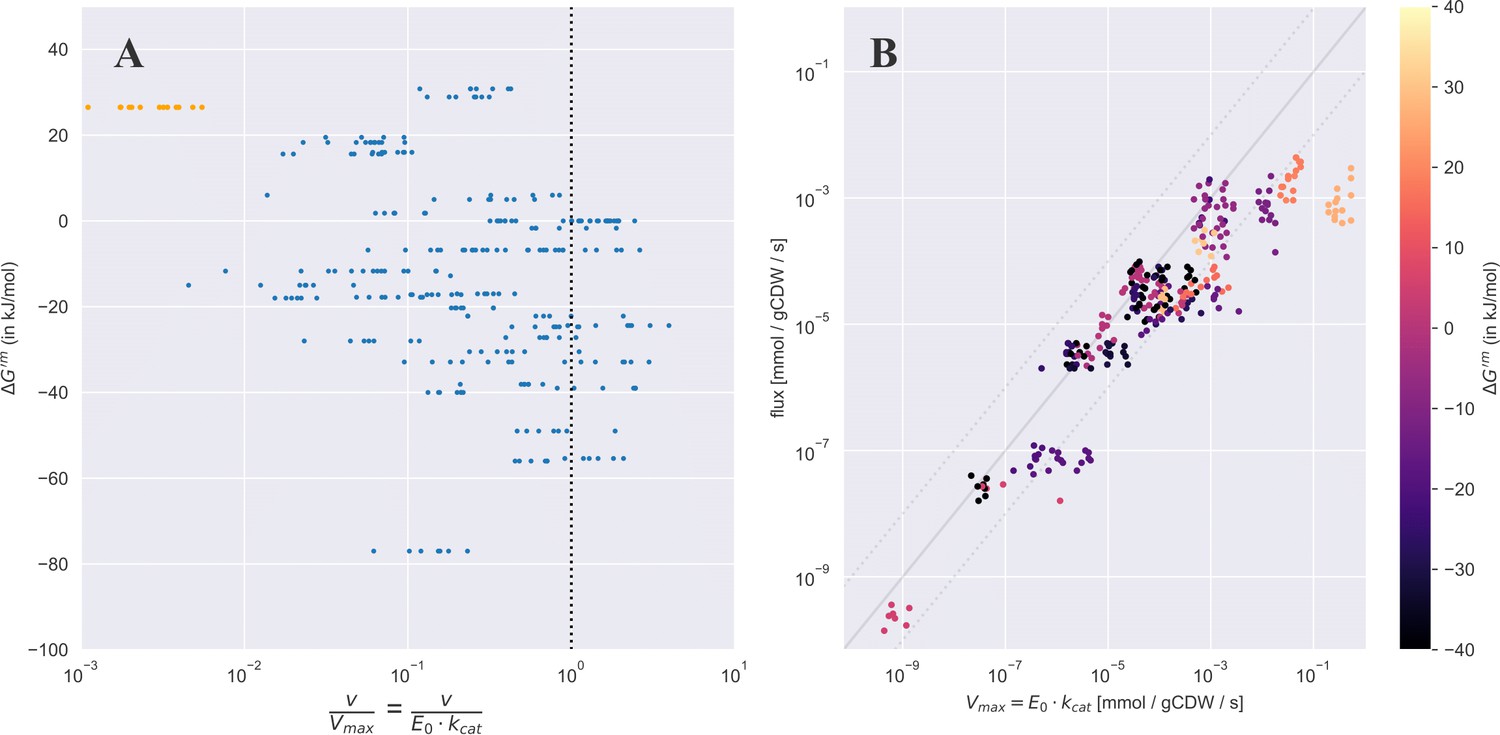
Measured flux values (from Davidi et al., 2016; Gerosa et al., 2015) plotted against $Δ G^{', m}$ which is the standard Gibbs energy of the reaction assuming all metabolites are at 1 mM concentrations (note this can be different than the usual definition of $Δ G^{', \circ}$ where concentrations are set to 1 M – a concentration that is not reflective of standard physiological conditions).

(A) shows a scatter plot of the ratio between the observed flux and the enzyme kinetic based limit ( $V_{m a x}$ ) against the $Δ G^{', m}$ . The points highlighted in orange are for the malate dehydrogenase reaction. (B) A scatter plot of the enzyme kinetic based limit against the measured flux (same data as in Figure 3 of the main text), where the $Δ G^{', m}$ is shown using a colourmap.

Appendix 8—figure 4

Download asset Open asset

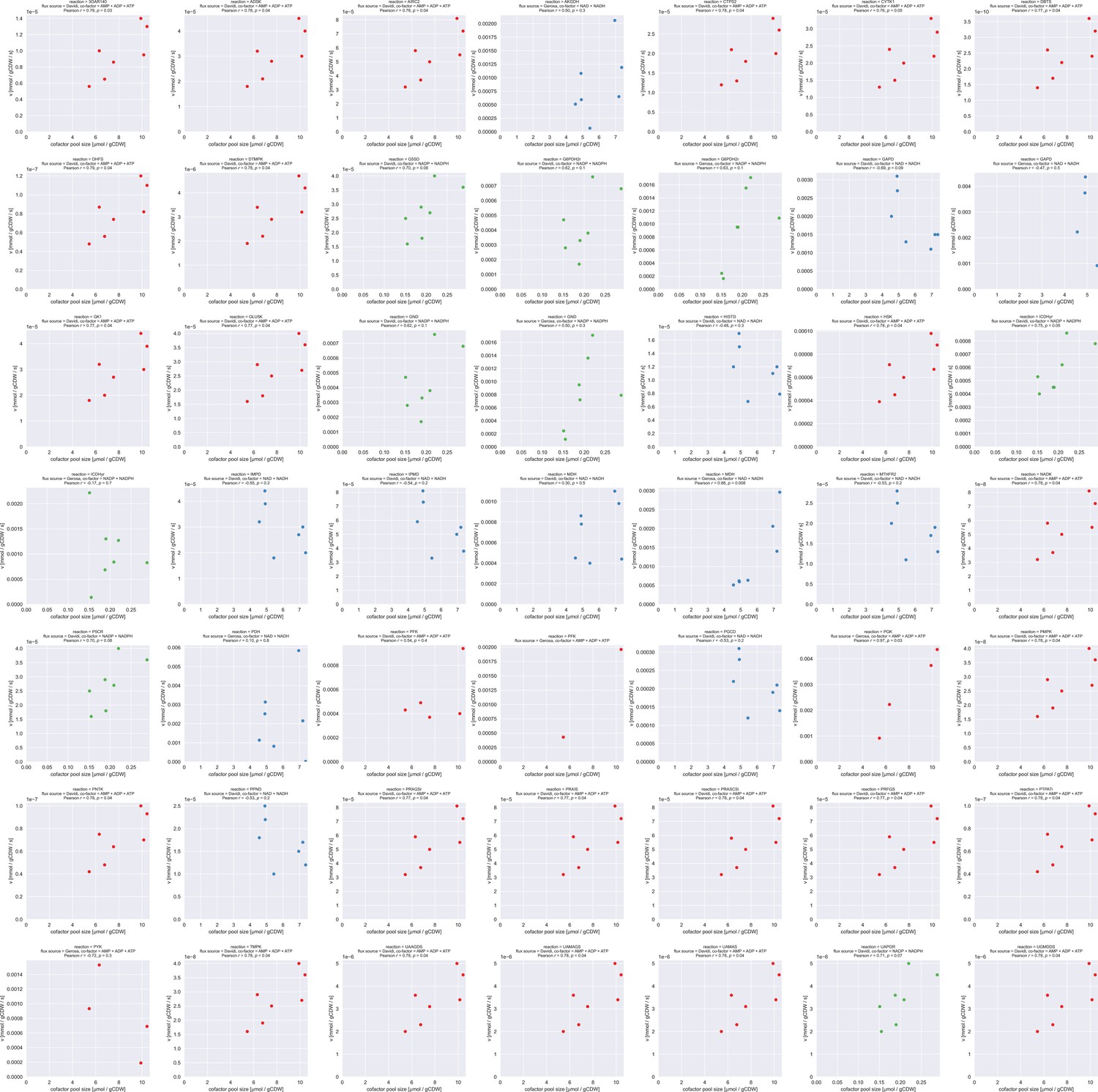
Measured flux values under different experimental conditions (from Davidi et al., 2016; Gerosa et al., 2015) for select reactions plotted against the corresponding co-substrate pool size.

See Supplementary file 1 for short notations for reactions. Each point on each panel is a separate flux measurement under a different environmental condition, where the co-substrate pool size is also measured. Point colours represent co-substrate type, with red for AMP +ADP + ATP, blue for NAD +NADH, and green for NADP +NADPH. Normalised RMSE of the best linear fit and the p-value are shown in the panel title.

Appendix 9—figure 1

Download asset Open asset

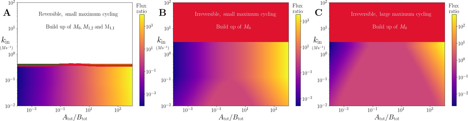
Effect of varying $A_{tot} / B_{tot}$ and k_in in the branching system shown in Figure 4A, on the ratio of flux into $M_{2, 2} / M_{2, 1}$ for reversible and irreversible dynamics and different $V_{\max, A}$ and $V_{\max, B}$ values.

Downstream metabolite has higher flux when it’s respective co-substrate has a higher concentration. (A) Reversible reactions with $V_{\max, A} = V_{\max, B} = 0.1$ (i.e. one order of magnitude smaller than the other reaction rates). (B) Irreversible reactions with $V_{\max, A} = V_{\max, B} = 0.1$ (i.e. one order of magnitude smaller than the other reaction rates). (C) Reversible reactions with $V_{\max, A} = V_{\max, B} = 10$ (i.e. one order of magnitude larger than the other reaction rates).

Appendix 9—figure 2

Download asset Open asset

Effect of varying $V_{\max, B} / V_{\max, A}$ (i.e maximum back-cycling) ratio and k_in in the branching system shown in Figure 4A.

(A) Motif showing the dynamics. (B) Heatmap showing the ratio of flux into $M_{2, 2} / M_{2, 1}$ . Downstream metabolite has higher flux when the back-cycling rate of its co-substrate is higher, with a greater effect for higher k_in values. (C) Time series of downstream metabolites and shared precursor. Solid/dashed lines show parameters for black/white dot in (B).

Appendix 10—figure 1

Download asset Open asset

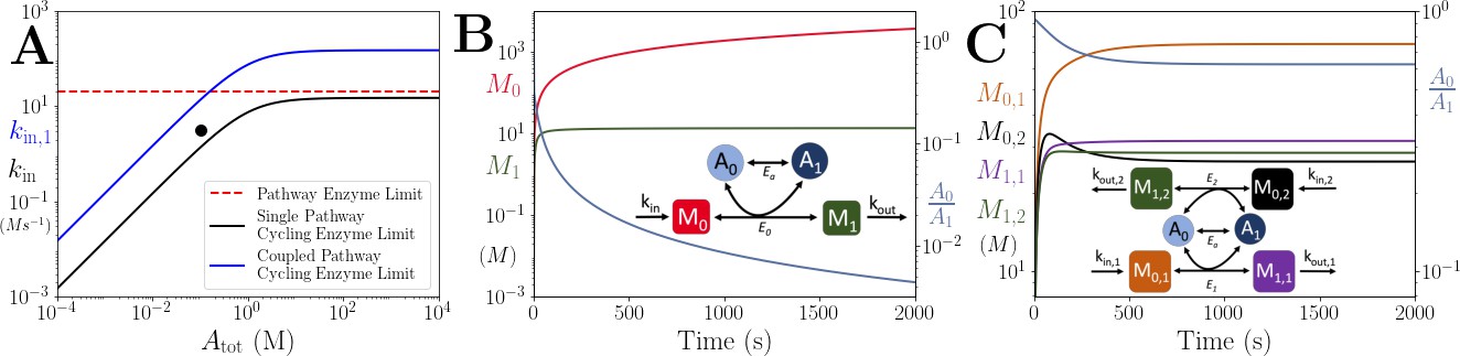
Comparison of the onset of instability in the coupled pathway case vs the single pathway case.

(A) Pathway enzyme and cycling enzyme limits in the single and coupled pathway cases (see legend, pathway enzyme limit is the same for each case). For the coupled pathway, $k_{in, 2}$ is set to. $0.9 k_{in, 1}$ Since the limiting factor depends on the difference between $k_{in, 1}$ and $k_{in, 2}$ , higher $k_{in}$ values are possible without build up of upstream metabolites if all other parameters are kept the same. (B) Time series of M₀, M₁ and $A_{0} / A_{1}$ in the single pathway case where the parameters for $A_{tot}$ and $k_{in}$ are set by the black dot in (A). Here we see build up M₀ because $k_{in} > A_{t o t} F_{a} / (A_{t o t} + L_{a})$ . (C) Time series of $M_{0, 1}$ , $M_{0, 2}$ , $M_{1, 1}$ , $M_{1, 2}$ and $A_{0} / A_{1}$ in the coupled pathway case where the parameters for $A_{tot}$ , $k_{in, 1}$ and $k_{in, 2}$ are set by the black dot in (A). Here we see the system admits a steady state because. $k_{i n, 1} - k_{i n, 2} < A_{t o t} F_{a} / (A_{t o t} + L_{a})$ The parameters in all panels are: $\frac{A_{t o t} F_{a}}{A_{t o t} L_{a}} > k_{i n, 1} - k_{i n, 2} > m a x (- \frac{A_{t o t} E_{a}}{A_{t o t} K_{a}}, \frac{E_{a} L_{a} + F_{a} K_{a}}{(K_{a} - L_{a})})$ , $K_{1} = L_{0} = K_{1, 1} = K_{1, 2} = L_{0, 1} = L_{0, 2} = 1 M$ , $k_{out} = k_{out, 1} = k_{out, 2} = 0.1 s^{- 1}$ , $E_{a} = F_{a} = 15 M s^{- 1}$ . $K_{a} = L_{a} = 1 M .$

Appendix 10—figure 2

Download asset Open asset

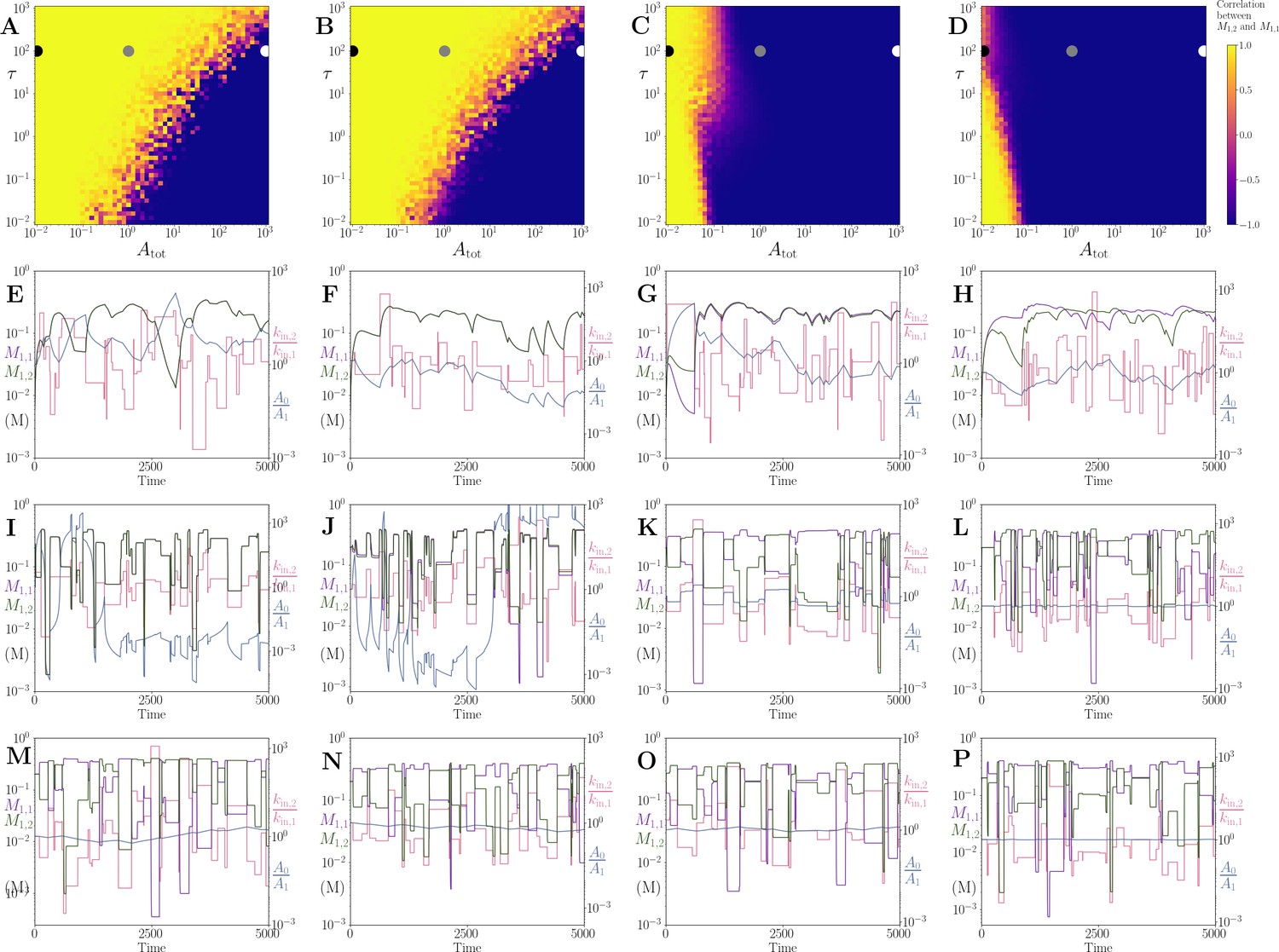
Correlation between products of two coupled pathways, using a model with irreversible reaction rates.

(A) - (D) show results for $E_{a} = F_{a} = 0, 0.01, 1$ and 10, respectively. As in the Figure 5 of the main text, all other parameters are set to 1, apart from the $k_{out}$ values that are each 0.5. As $E_{a}$ increases, the products become anti-correlated at smaller $A_{tot}$ values. This is also true for the model using reversible reaction rates (see Figure 5 of the main text). (E) - (P) show time series for the products $M_{1, 1}$ and $M_{1, 2}$ (purple and green respectively) on the left axis and the ratios $A_{0} / A_{1}$ and $k_{in, 2} / k_{in, 1}$ (blue and pink respectively) on the right axis. Panels in the same column share the same $E_{a}$ value as the heatmap in the top (*e.g*. $E_{a} = 0$ in (E), (I) and (M)). Panels (E) - (H), (I) - (L) and (M) - (P) have $A_{tot}$ and $τ$ given by the black, grey and white dots respectively. See text.

Tables

Appendix 8—table 1

Correlation coefficients between observed flux (measured or FBA-predicted) and co-substrate pool size.

For reaction ID and descriptions, see Supplementary file 1.

	Reaction	Flux source	Number of conditions	Pearson-r	p-Value
25	MDH	Gerosa	7	0.874310	0.010042
33	PGK	Gerosa	4	0.973547	0.026453
0	3OAR140	Davidi	7	0.794377	0.032850
7	DHFS	Davidi	7	0.787719	0.035438
46	UAMAS	Davidi	7	0.783767	0.037025
45	UAMAGS	Davidi	7	0.783767	0.037025
44	UAAGDS	Davidi	7	0.783767	0.037025
48	UGMDDS	Davidi	7	0.783767	0.037025
2	AIRC2	Davidi	7	0.783523	0.037125
39	PRASCSi	Davidi	7	0.783523	0.037125
27	NADK	Davidi	7	0.783523	0.037125
19	HSK	Davidi	7	0.783042	0.037321
4	CTPS2	Davidi	7	0.782303	0.037624
41	PTPATi	Davidi	7	0.781795	0.037833
35	PNTK	Davidi	7	0.781795	0.037833
8	DTMPK	Davidi	7	0.780177	0.038501
43	TMPK	Davidi	7	0.777454	0.039643
34	PMPK	Davidi	7	0.777454	0.039643
1	ADSK	Davidi	7	0.777418	0.039658
15	GLU5K	Davidi	7	0.774461	0.040918
37	PRAGSr	Davidi	7	0.773900	0.041159
40	PRFGS	Davidi	7	0.773900	0.041159
38	PRAIS	Davidi	7	0.773900	0.041159
14	GK1	Davidi	7	0.772918	0.041584
6	DBTS	Davidi	7	0.771900	0.042026
5	CYTK1	Davidi	7	0.762125	0.046410
20	ICDHyr	Davidi	7	0.743003	0.055681
47	UAPGR	Davidi	7	0.702799	0.078196
9	G5SD	Davidi	7	0.692830	0.084415
28	P5CR	Davidi	7	0.692830	0.084415
12	GAPD	Davidi	7	–0.681203	0.091988
11	G6PDH2r	Gerosa	7	0.629982	0.129423
10	G6PDH2r	Davidi	7	0.617909	0.139204
16	GND	Davidi	7	0.617909	0.139204
22	IMPD	Davidi	7	–0.539918	0.210941
23	IPMD	Davidi	7	–0.535973	0.214953
36	PPND	Davidi	7	–0.520516	0.231016
26	MTHFR2	Davidi	7	–0.519049	0.232569
32	PGCD	Davidi	7	–0.517475	0.234241
3	AKGDH	Gerosa	7	0.498666	0.254643
17	GND	Gerosa	7	0.498636	0.254676
42	PYK	Gerosa	4	–0.718821	0.281179
18	HISTD	Davidi	7	–0.469323	0.288020
30	PFK	Davidi	5	0.537260	0.350444
24	MDH	Davidi	7	0.311471	0.496502
13	GAPD	Gerosa	4	–0.451817	0.548183
21	ICDHyr	Gerosa	7	–0.169510	0.716347
29	PDH	Gerosa	7	0.098015	0.834403
31	PFK	Gerosa	2	nan	nan

Appendix 11—table 1

List of parameters together with the biological meanings and units.

M and t stand for Molar and time, respectively. Where different notation is used between this and the main text, the equivalent parameters have been made clear.

Parameter	Biological meaning and notes	Units
$E_{i}$ , $F_{i}$	Catalytic rate coefficients for forward and backward reactions respectively. In the main text we only use the forward rate and denote it $V_{\max, E_{i}}$ .	$M t^{- 1}$
$K_{i}$ , $L_{i - 1}$	Michaelis-Menten coefficients for forward and backward reactions, respectively. In the main text, we only use the forward rate and denote it $K_{M, E_{i}}$ .	$M^{n}$ , where $n$ is the number of different substrates involved in the reaction.
$k_{in}$	Influx rate.	$M t^{- 1}$
$k_{out}$	Outflow rate.	$t^{- 1}$

Additional files

Supplementary file 1 Enzyme kinetics, flux, metabolite concentration, and enzyme abundance data associated with flux analyses.: https://cdn.elifesciences.org/articles/84379/elife-84379-supp1-v2.xls
Download elife-84379-supp1-v2.xls
MDAR checklist: https://cdn.elifesciences.org/articles/84379/elife-84379-mdarchecklist1-v2.pdf
Download elife-84379-mdarchecklist1-v2.pdf

Download links

A two-part list of links to download the article, or parts of the article, in various formats.

Downloads (link to download the article as PDF)

Article PDF

Open citations (links to open the citations from this article in various online reference manager services)

Mendeley

Cite this article (links to download the citations from this article in formats compatible with various reference manager tools)

Robert West
Hadrien Delattre
Elad Noor
Elisenda Feliu
Orkun S Soyer

(2023)

Dynamics of co-substrate pools can constrain and regulate metabolic fluxes

eLife 12:e84379.

https://doi.org/10.7554/eLife.84379

Share this article

Cite this article

Motif, time-series and threshold in a single co-substrate involving reaction.

Motif, time-series and thresholds for the linear pathway model with n=4.

Measured and FBA-predicted flux values are typically lower than the calculated primary enzyme threshold.

Motif, heatmap and time-series for the branching pathway model.

Figure 4—source code 1

Motif, heatmap and time-series for the coupled pathway model with noisy influxes.

Figure 5—source code 1

Cartoon representation of select metabolic pathways involving co-substrate cycling.

Concentrations of non-accumulating metabolites vs kin in the models presented in Figures 1 and 2 of the main text.

Motif, time series and threshold for the linear pathway model with multiple co-substrates.

Motif, time series and threshold for a model with differential co-substrate stoichiometry, as seen in glycolysis.

Motif, time series and threshold for model with both co-substrate and metabolite cycling, mimicking nitrogen assimilation.

Measured flux values (from Davidi et al., 2016; Gerosa et al., 2015) plotted against the calculated primary enzyme kinetic threshold (first part of Eq. (1) of the main text) adjusted by substrate affinity of the enzyme.

Cumulative distribution of the ratio of observed flux (measured or FBA-predicted) to enzyme kinetic based limit (Vmax) (left panel) or to enzyme kinetic based limit accounting for substrate affinity (right panel).

Measured flux values under different experimental conditions (from Davidi et al., 2016; Gerosa et al., 2015) for select reactions plotted against the corresponding co-substrate pool size.

Effect of varying Atot/Btot and kin in the branching system shown in Figure 4A, on the ratio of flux into M2,2/M2,1 for reversible and irreversible dynamics and different Vmax,A and Vmax,B values.

Effect of varying Vmax,B/Vmax,A (i.e maximum back-cycling) ratio and kin in the branching system shown in Figure 4A.

Comparison of the onset of instability in the coupled pathway case vs the single pathway case.

Correlation between products of two coupled pathways, using a model with irreversible reaction rates.

Correlation coefficients between observed flux (measured or FBA-predicted) and co-substrate pool size.

List of parameters together with the biological meanings and units.

Supplementary file 1

MDAR checklist

Downloads (link to download the article as PDF)

Open citations (links to open the citations from this article in various online reference manager services)

Cite this article (links to download the citations from this article in formats compatible with various reference manager tools)

Motif, time-series and thresholds for the linear pathway model with $n = 4$ .

Concentrations of non-accumulating metabolites vs k_in in the models presented in Figures 1 and 2 of the main text.

Cumulative distribution of the ratio of observed flux (measured or FBA-predicted) to enzyme kinetic based limit ( $V_{\max}$ ) (left panel) or to enzyme kinetic based limit accounting for substrate affinity (right panel).

Effect of varying $A_{tot} / B_{tot}$ and k_in in the branching system shown in Figure 4A, on the ratio of flux into $M_{2, 2} / M_{2, 1}$ for reversible and irreversible dynamics and different $V_{\max, A}$ and $V_{\max, B}$ values.

Effect of varying $V_{\max, B} / V_{\max, A}$ (i.e maximum back-cycling) ratio and k_in in the branching system shown in Figure 4A.