The genomic footprint of social stratification in admixing American populations
- Department of Life Sciences, Silwood Park Campus, Imperial College London, United Kingdom
- Department of Statistical Sciences, University of Bologna, Italy
- Department of Computer Science, Haverford College, United States
- School of Biological and Behavioural Sciences, Queen Mary University of London, United Kingdom
Figures
Figure 1 with 1 supplement
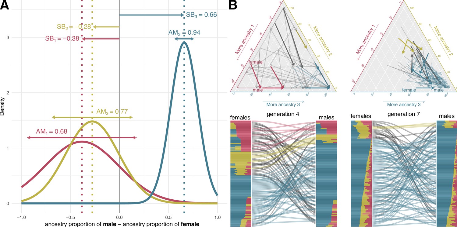
Mating model.
(A) Assortative mating (AM) and sex bias (SB) values that modulate the mating probabilities in a simulation example of 19 generations from the colonization of America to nowadays. The mating probability for a given couple is set as a function of the differences in the genetic ancestry proportions for each ancestry. We assume the mating probability follow a three-dimensional normal distribution. In this normal distribution, SB sets the expected value and AM is inversely proportional to its variance. (B) Ancestry proportions of mating couples at generations 4 and 7 in ternary plots (top) and barplots (bottom) based on the mating probabilities defined in A. In the top plots, each arrow represents a couple. The arrow tail and head coordinates in the ternary plots show the ancestry proportions of the female and the male, respectively. In the bottom, the barplots represent male and female ancestry proportions, linked by curved lines reflecting mating. Red, yellow, and blue correspond to ancestries 1, 2, and 3. The arrows in the ternary plot and the lines between barplots representing a mating couple are colored with the color corresponding to the predominant ancestry in both male and female, and they are depicted in black if it differs between them.
Figure 1—figure supplement 1
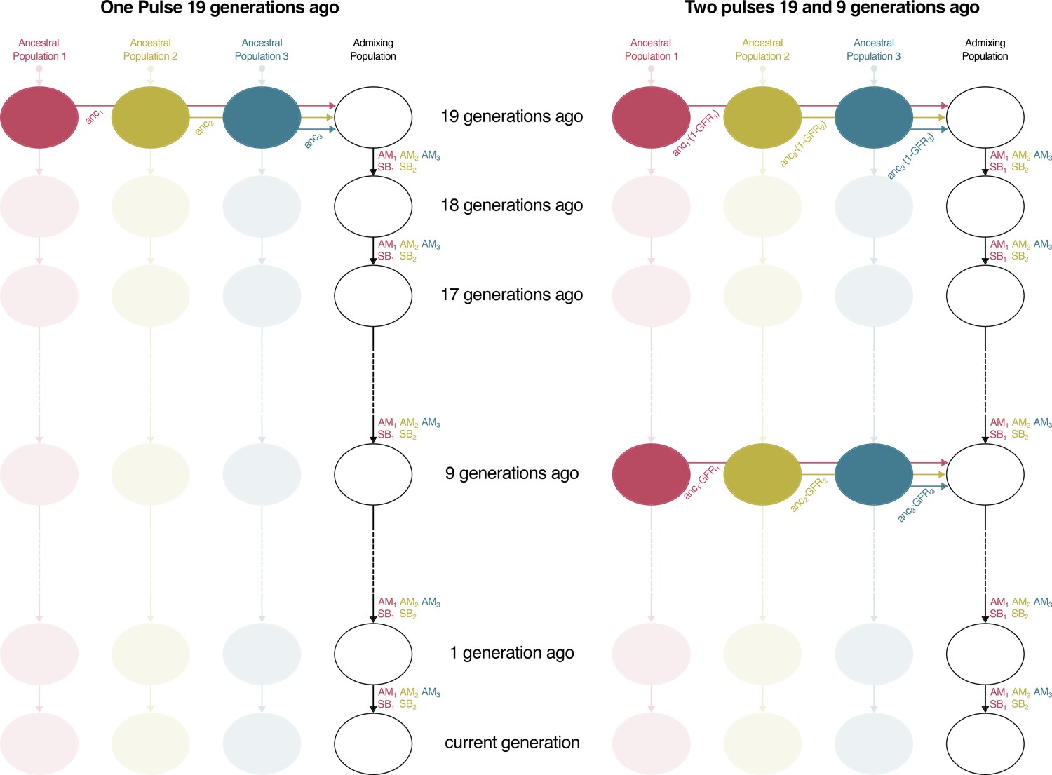
Admixture Model for One Pulse and Two Pulses.
In the One Pulse model, the first generation of the admixing population is formed 19 generations ago by a migration pulse from the ancestral population that equals the ancestry proportions observed in the studied population. In the Two Pulses model, an extra pulse is modeled 9 generations ago. The proportion of migrants that arrive in the second pulse is modeled by gene flow rate (GFR). In the admixing population, there is no random mating from one generation to the other, but mating is constrained by the mating parameters (AM1, AM2, AM3, SB1 and SB2).
Figure 2 with 6 supplements
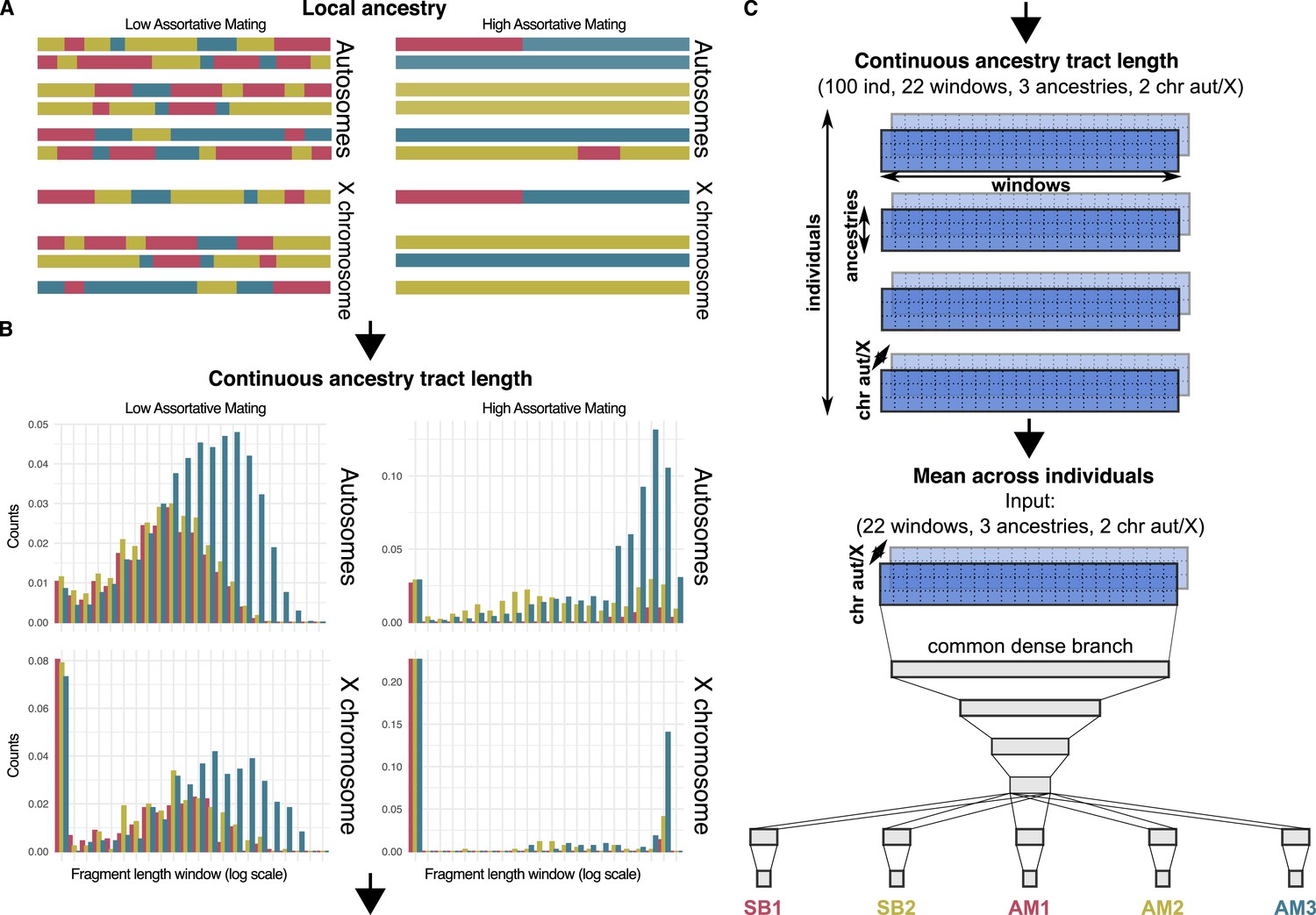
Local ancestry, Contiuous ancestry tract length and Neural network.
(A) Schematic view of the autosomal and sex chromosomes split into the continuous ancestry tracts inherited from each of the three ancestries after a local ancestry analysis with RFMix. (B) Continuous ancestry tract length profile displaying the number of tracts for each ancestry in each tract length bin. The break points that define the bin widths are set in a logarithmic scale. (C) Matrix representing the continuous ancestry tract length profile accounting for the amount of tracts in each length bin, for each ancestry in either autosomal or sex chromosome for each individual. The mean across individuals summarises the four-dimensional matrix in a population three-dimensional matrix, which is used as the input of the neural network. The neural network has four fully connected layers that split into a branch for each parameter, each one made of a last hidden layer connected to the output layer.
Figure 2—figure supplement 1
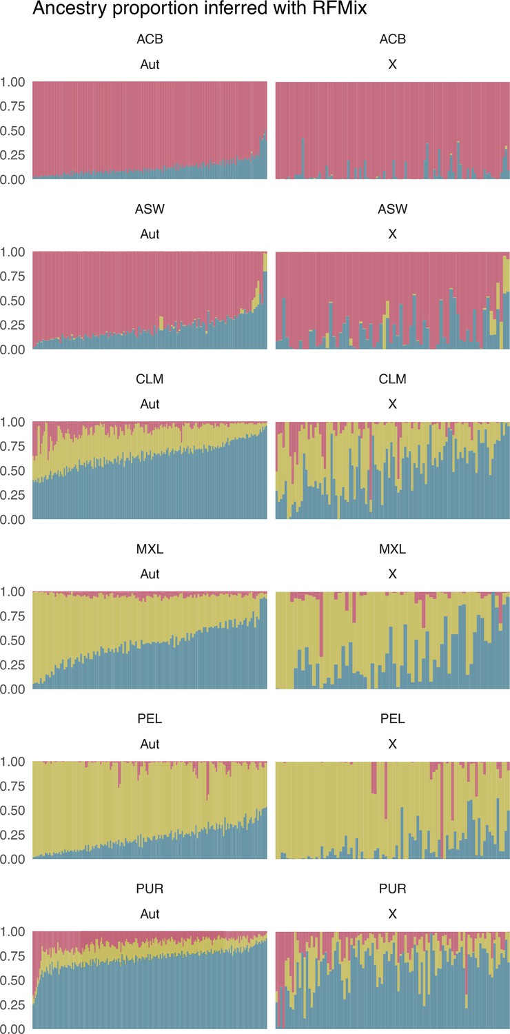
Individual proportions of sub-Saharan (red), Native American (green), and European (blue) ancestry were inferred after a Local Ancestry analysis with RFMix for autosomes (Aut), on the left, and X chromosome (X), on the right, for each population.
Each vertical bar represents an individual. Individuals are sorted along the x-axis based on the autosomal proportions inferred with RFMix in both autosomes and X chromosome plots.
Figure 2—figure supplement 2
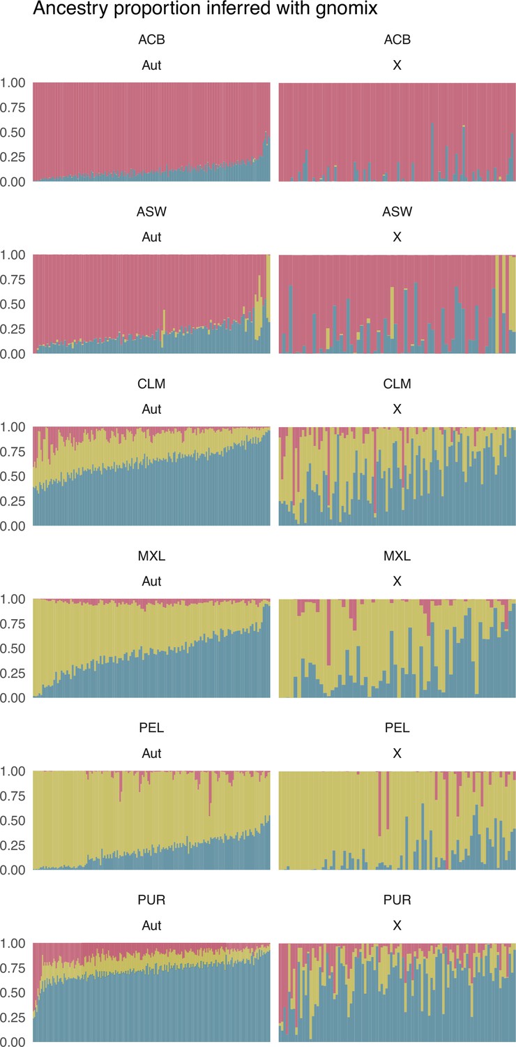
Individual proportions of sub-Saharan (red), Native American (green), and European (blue) ancestry inferred after a Local Ancestry analysis with Gnomix for autosomes (Aut), on the left, and X chromosome (X), on the right, for each population.
Each vertical bar represents an individual. Individuals are sorted along the x-axis based on the autosomal proportions inferred with RFMix in both autosomes and X chromosome plots.
Figure 2—figure supplement 3
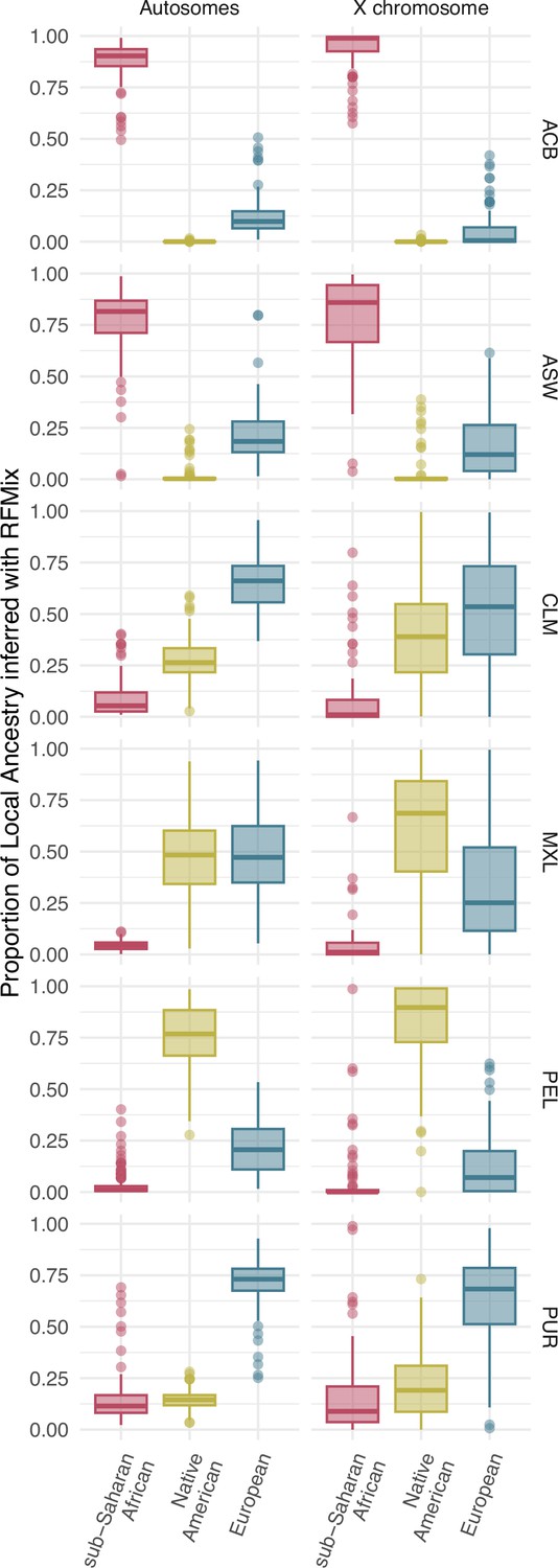
Distribution of individual proportions of sub-Saharan (red), Native American (green), and European (blue) ancestry inferred after a Local Ancestry analysis with RFMix for autosomes (Aut), on the left, and X chromosome (X), on the right, for each population. The box limits are the 25th and 75th percentiles and the points show the outliers 1.5 times the interquartile range above the 75th percentile and below the 25th percentile.
Figure 2—figure supplement 4
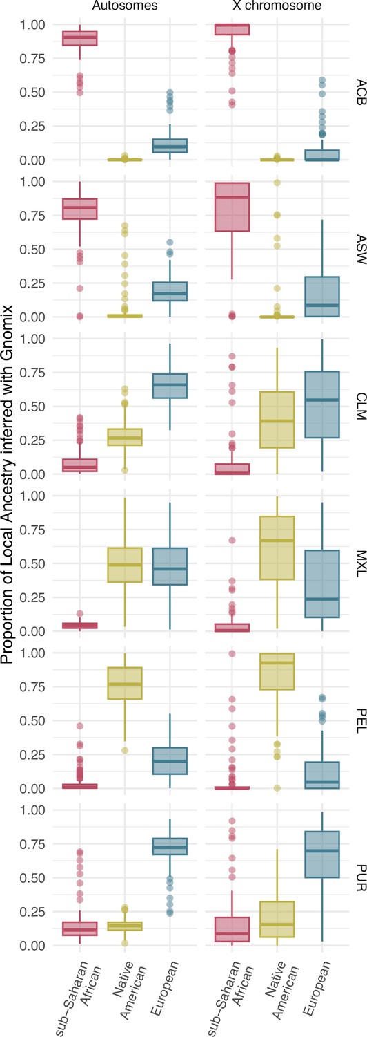
Distribution of individual proportions of sub-Saharan (red), Native American (green), and European (blue) ancestry inferred after a Local Ancestry analysis with Gnomix for autosomes (Aut), on the left, and X chromosome (X), on the right, for each population. The box limits are the 25th and 75th percentiles and the points show the outliers 1.5 times the interquartile range above the 75th percentile and below the 25th percentile.
Figure 2—figure supplement 5
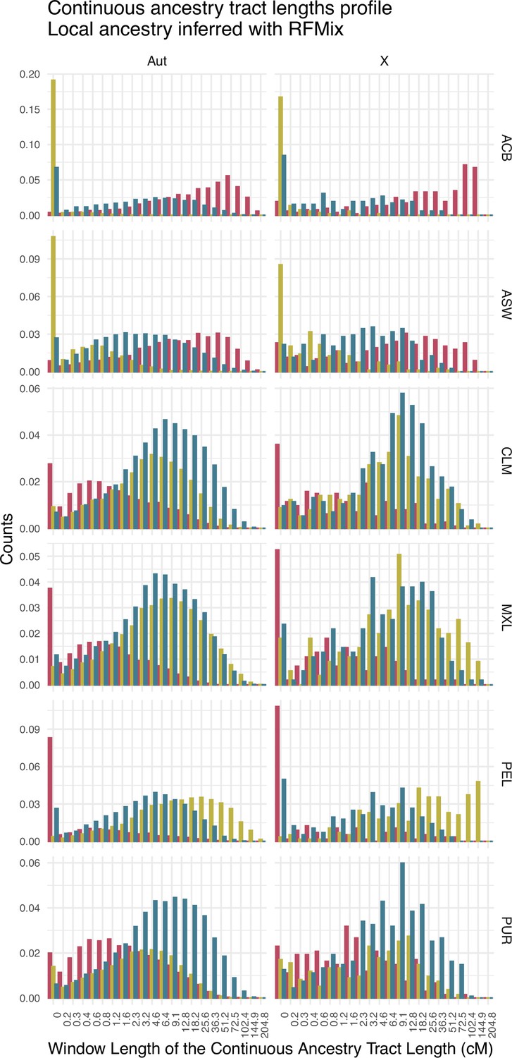
Continuous ancestry tract lengths profile showing the amount of fragments in each length window for sub-Saharan (red), Native American (green), and European (blue) ancestry for each population, after a local ancestry analysis with RFMix.
Figure 2—figure supplement 6
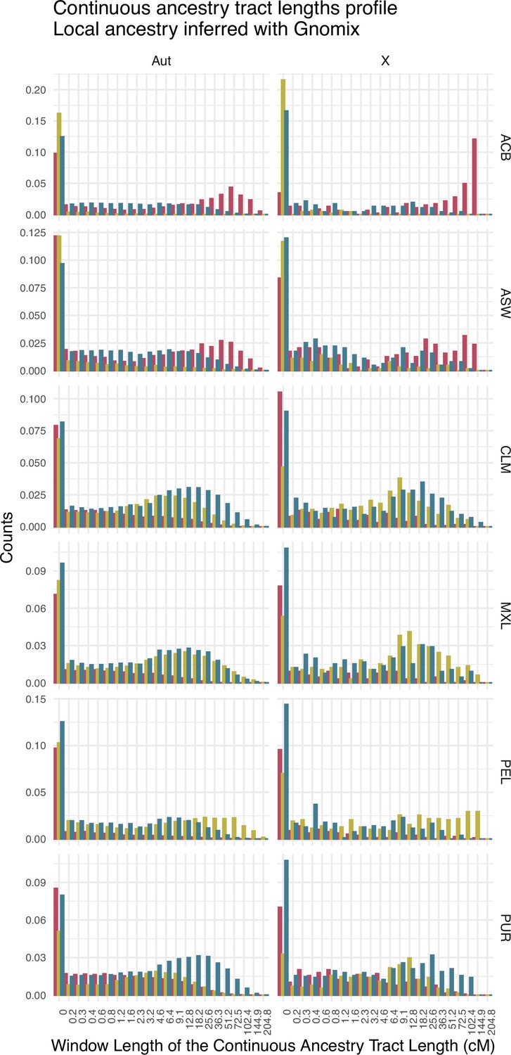
Continuous ancestry tract lengths profile showing the amount of fragments in each length window for sub-Saharan (red), Native American (green), and European (blue) ancestry for each population, after a local ancestry analysis with Gnomix.
Figure 3 with 2 supplements
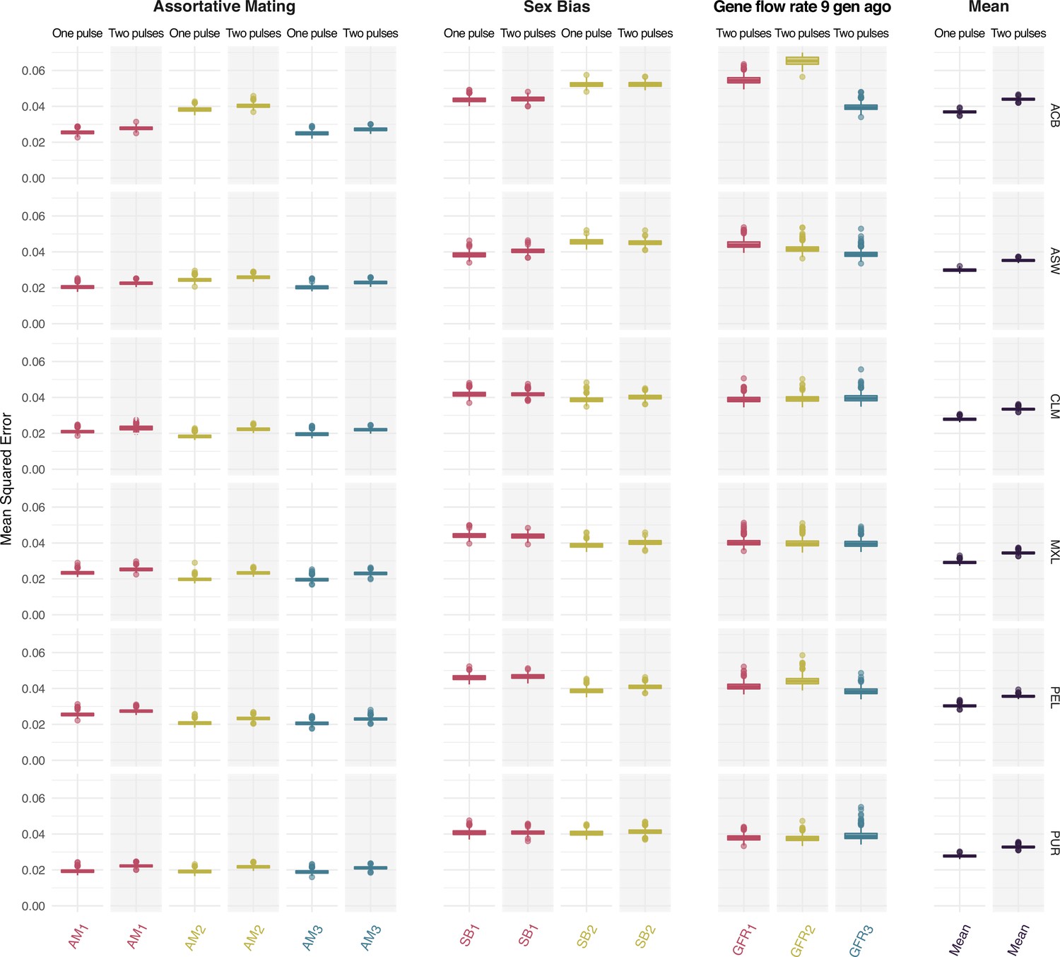
Mean squared error comparing true and predicted values at testing for the assortative mating, sex bias, gene flow rate 9 generations ago parameters for each ancestry for both One Pulse and Two Pulses models and mean values for each model.
Each color represents the values for a different ancestry (red, yellow, and blue for ancestries 1, 2, and 3 respectively, which correspond to sub-Saharan, Native American and European ancestries). The boxplot shows the distributions of values across the 1000 trained neural networks. The box limits are the 25th and 75th percentiles and the points show the outliers 1.5 times the interquartile range above the 75th percentile and below the 25th percentile.
Figure 3—figure supplement 1
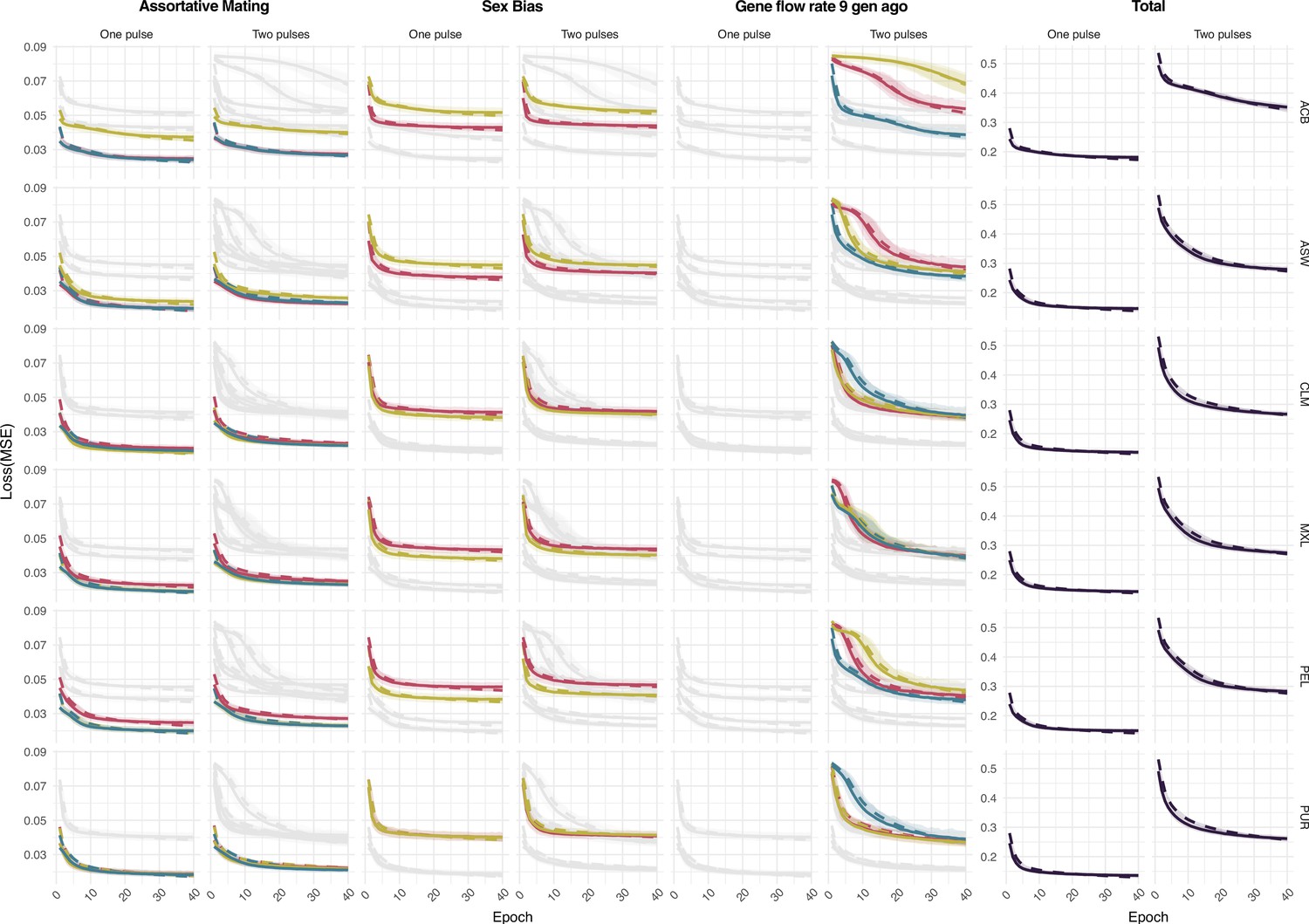
Loss function at training for the assortative mating, sex bias, gene flow rate 9 generations ago parameters for each ancestry for both One Pulse and Two Pulses models and mean values for each model.
Each color is related to a different ancestry as in Figure 3.
Figure 3—figure supplement 2
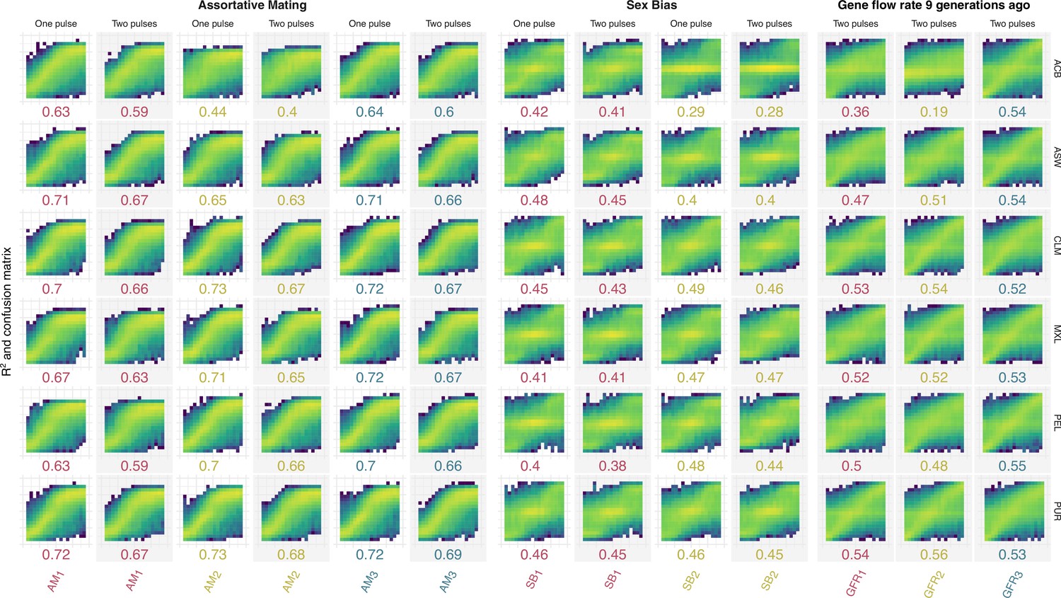
Confusion matrices and R2 comparing true (x-axis) and predicted (y-axis) values at testing for assortative mating, sex bias, gene flow Rate 9 generations ago parameters for each ancestry for both One Pulse and Two Pulses models.
Each color is related to a different ancestry as in Figure 3.
Figure 4 with 7 supplements
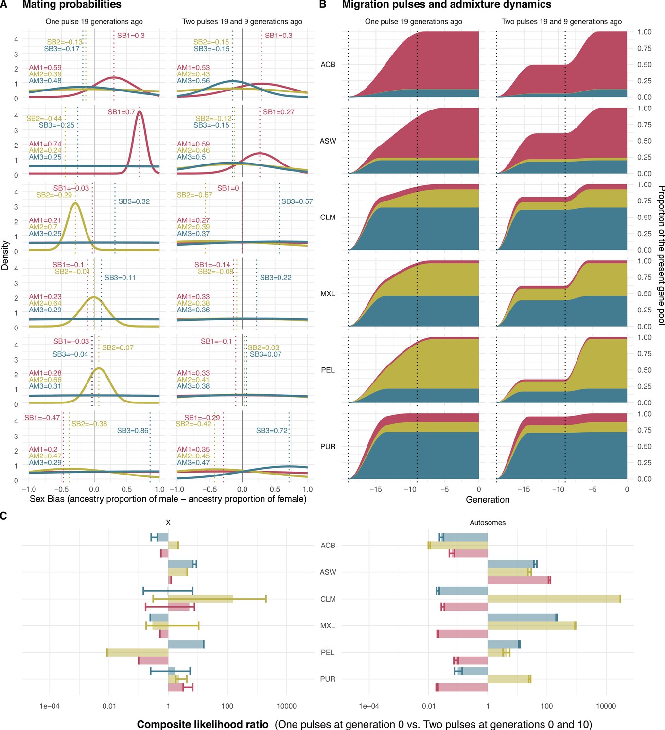
Mating probabilities, migration pulses and admixture dynamics.
(A) Mating probabilities as a function of male and female proportions of each ancestry, for each population. (B) Migration pulses of each ancestry according to scenarios allowing One Pulse and Two Pulses for each population. The y-axis represents the cumulative increase in the ancestry-specific gene pool relative to the final ancestry proportions, at each generation. The ancestry proportions at generation 19 represent the observed ancestry proportions of each population in real data. The increase in the cumulative ancestry-specific gene pool is defined by gene flow rate (GFR), while the slope of the increase is represented inversely proportional to assortative mating (AM). (C) Composite likelihood ratio comparing Two Pulses model vs. One Pulse model, for each ancestry for both the X chromosome and the autosomes. In this plot, positive values show a higher likelihood of the Two Pulses model based on the fit of the real fragment lengths in the distribution of fragment lengths of simulated data under the AM and sex bias (SB) parameters predicted by the neural network. Error bars define the 95% CI obtained by bootstrapping the tract lengths profile.
Figure 4—figure supplement 1
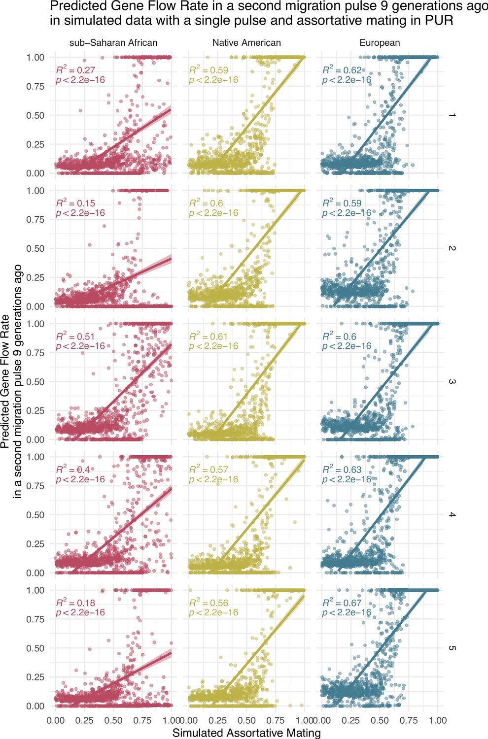
Correlation between simulated assortative mating (AM) values and predicted gene flow rate (GFR) values (Simulation only for PUR, due to large computational requirements).
The Neural network for the Two Pulses model has been trained with Two Pulses simulations, but once trained it has been used to predict GFR from the output tract length of simulations of the One Pulse model that only iterates AM1, AM2, and AM3 but keeps SB1 and SB2 equal to 0. Each of the five rows of plots represents a different training of the neural network.
Figure 4—figure supplement 2
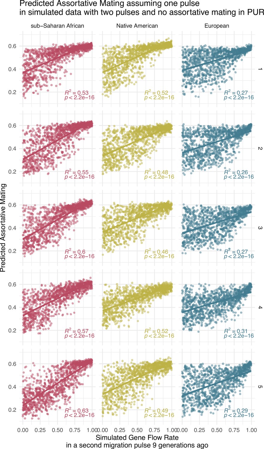
Correlation between simulated gene flow rate (GFR) values and predicted assortative mating (AM) values (Simulation only for PUR, due to large computational requirements).
The Neural network for the One Pulse model has been trained with One Pulse simulations, but once trained it has been used to predict AM from the output tract length of simulations of the Two Pulses model that only iterates GFR1, GFR2, and GFR3 but keeps SB1, SB2, AM1, AM2, and AM3 equal to 0. Each of the five rows of plots represents a different training of the neural network.
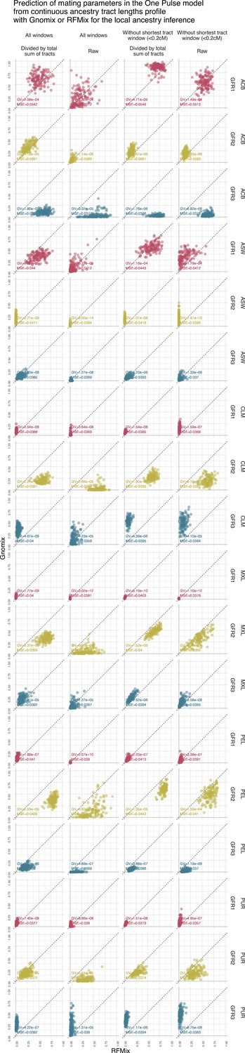
Figure 4—figure supplement 3
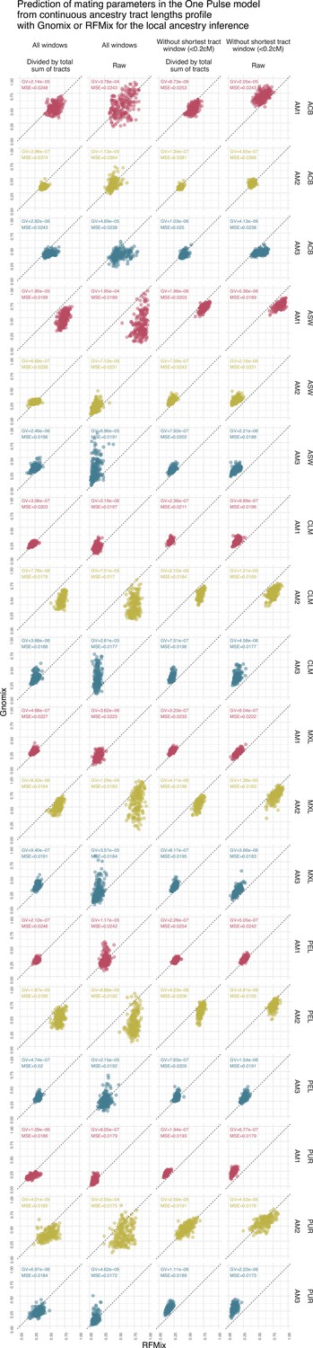
Prediction of assortative mating in the One Pulse model using the continuous ancestry tract lengths profile from Gnomix or RFMix.
Each point is the estimated parameter from each of the 1000 trainings using either RFMix or Gnomix tract length profile as input to the trained neural network. The tract length profile has been modified either by dividing each value by the total number of tracts or by removing the window corresponding to the shortest tracts, or both. We have evaluated the test MSE reported in Figure 3 and the genaralized variance (GV) in each case . Table 7 show mean GV and mean MSE for each tract length modification.
Figure 4—figure supplement 4
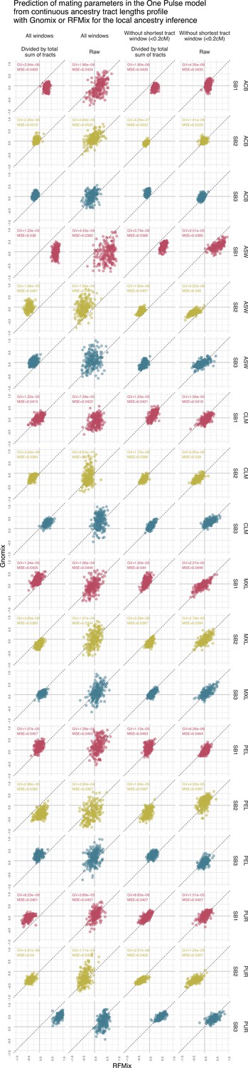
Prediction of sex bias in the One Pulse model using the continuous ancestry tract lengths profile from Gnomix or RFMix.
Each point is the estimated parameter from each of the 1000 trainings using either RFMix or Gnomix tract length profile as input to the trained neural network. The tract length profile has been modified either by dividing each value by the total number of tracts or by removing the window corresponding to the shortest tracts, or both. We have evaluated the test MSE reported in Figure 3 and the genaralized variance (GV) in each case . Table 8 show mean GV and mean MSE for each tract length modification.
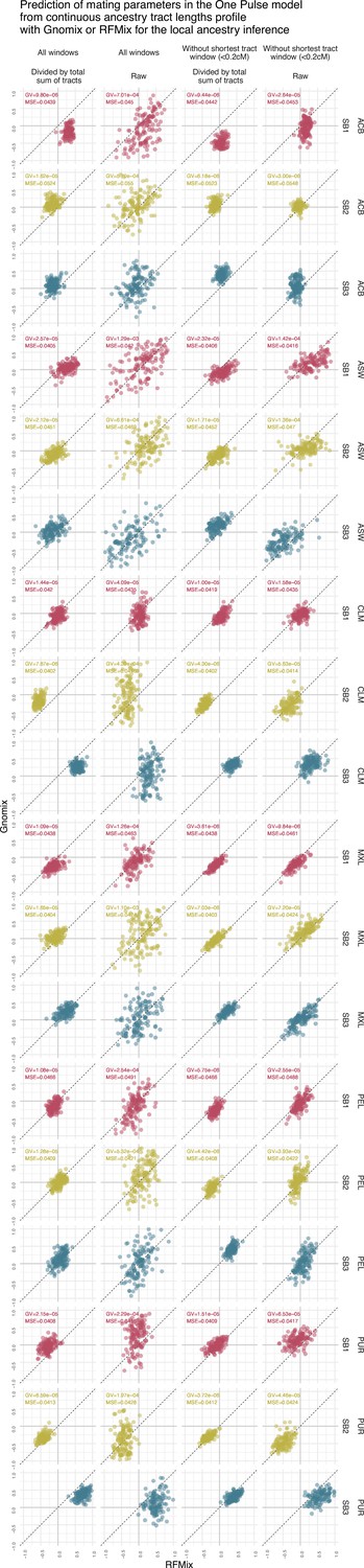
Figure 4—figure supplement 5
Prediction of assortative mating in the Two Pulses model using the continuous ancestry tract lengths profile from Gnomix or RFMix.
Each point is the estimated parameter from each of the 1000 trainings using either RFMix or Gnomix tract length profile as input to the trained neural network. The tract length profile has been modified either by dividing each value by the total number of tracts or by removing the window corresponding to the shortest tracts, or both. We have evaluated the test MSE reported in Figure 3 and the genaralized variance (GV) in each case . Table 8 show mean GV and mean MSE for each tract length modification.
Figure 4—figure supplement 6
Prediction of sex bias in the Two pulses model using the continuous ancestry tract lengths profile from Gnomix or RFMix.
Each point is the estimated parameter from each of the 1000 trainings using either RFMix or Gnomix tract length profile as input to the trained neural network. The tract length profile has been modified either by dividing each value by the total number of tracts or by removing the window corresponding to the shortest tracts, or both. We have evaluated the test MSE reported in Figure 3 and the genaralized variance (GV) in each case . Table 8 show mean GV and mean MSE for each tract length modification.
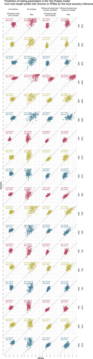
Figure 4—figure supplement 7
Prediction of gene flow rate in the Two Pulses model using the continuous ancestry tract lengths profile from Gnomix or RFMix.
Each point is the estimated parameter from each of the 1000 trainings using either RFMix or Gnomix tract length profile as input to the trained neural network. The tract length profile has been modified either by dividing each value by the total number of tracts or by removing the window corresponding to the shortest tracts, or both. We have evaluated the test MSE reported in Figure 3 and the genaralized variance (GV) in each case . Table 8 show mean GV and mean MSE for each tract length modification.
Tables
Table 1
Average proportions percentage (and 95% CI) of genetic ancestry for each population, inferred after a local ancestry analysis with RFMix.
| Population | Ancestry | Aut | X |
|---|---|---|---|
| ACB | AFR | 88.3 (75.9, 97.4) | 94 (72.6, 99.6) |
| ACB | NAT | 0.1 (0, 0.2) | 0.1 (0, 1) |
| ACB | EUR | 11.8 (2.8, 24.2) | 5.4 (0, 25.7) |
| ASW | AFR | 76.9 (49.9, 91.4) | 77.5 (39.7, 99.6) |
| ASW | NAT | 1.5 (0, 13.2) | 3.7 (0, 27.6) |
| ASW | EUR | 21.7 (8.7, 41.2) | 18.3 (0, 54.2) |
| CLM | AFR | 8.2 (1.4, 23.5) | 8 (0, 43.4) |
| CLM | NAT | 26.8 (10.5, 43.4) | 40.1 (4.8, 81.4) |
| CLM | EUR | 65.1 (41.6, 86.8) | 51.5 (12.5, 91.9) |
| MXL | AFR | 4.4 (1, 7.7) | 5.2 (0, 29.7) |
| MXL | NAT | 49.3 (23.3, 87.7) | 61.2 (11.4, 99.5) |
| MXL | EUR | 46.5 (11.5, 72.9) | 33.2 (0, 86.4) |
| PEL | AFR | 3.2 (0.1, 14) | 5.1 (0, 32.9) |
| PEL | NAT | 75.4 (50.5, 95.4) | 81.9 (37.3, 99.6) |
| PEL | EUR | 21.6 (4, 43) | 12.5 (0, 47.8) |
| PUR | AFR | 13.8 (4.8, 24.2) | 15.4 (0.3, 56.6) |
| PUR | NAT | 14.4 (7, 21.2) | 21.2 (0.4, 53.3) |
| PUR | EUR | 72 (56.1, 86.3) | 63 (21.9, 88.2) |
Table 2
Average proportions (%) of genetic ancestry for each population, inferred after a local ancestry analysis with Gnomix.
| PopulatioAn | ancestry | Aut | X |
|---|---|---|---|
| ACB | AFR | 88.5 (75.8, 97.6) | 93.6 (70.9, 99.5) |
| ACB | NAT | 0.1 (0, 0.5) | 0.1 (0, 0.4) |
| ACB | EUR | 11.4 (2.3, 23.7) | 5.9 (0, 28.6) |
| ASW | AFR | 77 (47.7, 91.7) | 76.2 (13.6, 99.5) |
| ASW | NAT | 3.8 (0, 24.2) | 5.7 (0, 55.5) |
| ASW | EUR | 19.3 (6.8, 36) | 17.6 (0, 65.3) |
| CLM | AFR | 7.9 (0.9, 24.4) | 7.8 (0, 51.6) |
| CLM | NAT | 27.1 (10, 44.9) | 39.1 (3, 84.8) |
| CLM | EUR | 65(41, 89) | 52.6 (8.4, 95.9) |
| MXL | AFR | 4.2 (0.8, 8.2) | 5.1 (0, 28.6) |
| MXL | NAT | 50(23, 87) | 60.2 (9.1, 99.5) |
| MXL | EUR | 45.8 (11.3, 73.9) | 34.1 (0, 87) |
| PEL | AFR | 3.1 (0, 13.5) | 5.1 (0, 33.2) |
| PEL | NAT | 77 (52.2, 98.2) | 81.6 (32.5, 99.5) |
| PEL | EUR | 19.9 (1.6, 40.6) | 12.8 (0, 51.3) |
| PUR | AFR | 13.5 (4.8, 25.1) | 15 (0, 56.1) |
| PUR | NAT | 14.3 (6.7, 21.5) | 20.4 (0, 60.7) |
| PUR | EUR | 72.2 (57.3, 87.9) | 64.1 (23.6, 93.1) |
Table 3
Estimated Mean (and 95 %CI) of the mating parameters for the One Pulse Model, using the continuous ancestry tract lengths profile obtained from RFMix as input to 1000 trained neural networks.
| Population | CLM | MXL | PEL | PUR | ASW | ACB |
|---|---|---|---|---|---|---|
| AM1 | 0.21 (0.17, 0.26) | 0.23 (0.19, 0.28) | 0.28 (0.25, 0.31) | 0.2 (0.13, 0.28) | 0.74 (0.64, 0.81) | 0.59 (0.48, 0.69) |
| AM2 | 0.7 (0.64, 0.76) | 0.64 (0.55, 0.71) | 0.66 (0.58, 0.74) | 0.47 (0.33, 0.62) | 0.24 (0.18, 0.31) | 0.39 (0.35, 0.44) |
| AM3 | 0.25 (0.2, 0.31) | 0.29 (0.24, 0.33) | 0.31 (0.27, 0.34) | 0.29 (0.21, 0.39) | 0.25 (0.19, 0.32) | 0.48 (0.41, 0.59) |
| SB1 | –0.03 (-0.28, 0.16) | –0.1 (-0.31, 0.1) | –0.03 (-0.18, 0.15) | –0.47 (−0.64, –0.25) | 0.7 (0.56, 0.81) | 0.3 (0.2, 0.4) |
| SB2 | –0.29 (−0.43, –0.17) | –0.01 (-0.15, 0.13) | 0.07 (-0.23, 0.26) | –0.38 (−0.54, –0.23) | –0.44 (−0.6, –0.31) | –0.13 (−0.23, –0.02) |
| SB3 | 0.32 (0.18, 0.49) | 0.11 (-0.03, 0.25) | –0.04 (-0.17, 0.13) | 0.86 (0.68, 1.01) | –0.25 (−0.41, –0.1) | –0.17 (−0.27, –0.08) |
Table 4
Estimated Mean (and 95 %CI) of the mating parameters for the One Pulse Model, using the continuous ancestry tract lengths profile obtained from Gnomix as input to 1000 trained neural networks.
| population | CLM | MXL | PEL | PUR | ASW | ACB |
|---|---|---|---|---|---|---|
| AM1 | 0.22 (0.18,0.26) | 0.26 (0.22,0.31) | 0.27 (0.24,0.31) | 0.16 (0.12,0.21) | 0.51 (0.33,0.65) | 0.51 (0.39,0.64) |
| AM2 | 0.45 (0.32,0.6) | 0.52 (0.38,0.64) | 0.48 (0.33,0.62) | 0.35 (0.24,0.49) | 0.26 (0.23,0.3) | 0.36 (0.32,0.4) |
| AM3 | 0.31 (0.24,0.44) | 0.34 (0.28,0.42) | 0.31 (0.27,0.37) | 0.23 (0.16,0.32) | 0.32 (0.26,0.39) | 0.4 (0.35,0.46) |
| SB1 | –0.01 (-0.24,0.2) | 0.17 (-0.04,0.41) | 0.12 (-0.1,0.36) | –0.08 (-0.28,0.08) | 0.01 (-0.35,0.31) | –0.08 (-0.29,0.11) |
| SB2 | –0.21 (−0.39,,–0.06) | –0.21 (−0.39,,–0.03) | –0.36 (−0.59,,–0.06) | –0.36 (−0.5,,–0.2) | –0.04 (-0.22,0.25) | 0.02 (-0.1,0.19) |
| SB3 | 0.21 (0.07,0.4) | 0.04 (-0.1,0.18) | 0.23 (0.04,0.39) | 0.44 (0.25,0.62) | 0.03 (-0.15,0.23) | 0.05 (-0.09,0.21) |
Table 5
Estimated Mean (and 95 %CI) of the mating parameters for the Two Pulses model, using the continuous ancestry tract lengths profile obtained from RFMix as input to 1000 trained neural networks.
| population | CLM | MXL | PEL | PUR | ASW | ACB |
|---|---|---|---|---|---|---|
| AM1 | 0.27 (0.22,0.34) | 0.33 (0.23,0.42) | 0.33 (0.25,0.44) | 0.35 (0.26,0.44) | 0.59 (0.45,0.73) | 0.53 (0.42,0.63) |
| AM2 | 0.39 (0.28,0.5) | 0.38 (0.28,0.48) | 0.41 (0.32,0.52) | 0.45 (0.32,0.6) | 0.46 (0.35,0.58) | 0.43 (0.36,0.52) |
| AM3 | 0.37 (0.29,0.45) | 0.36 (0.25,0.47) | 0.38 (0.3,0.47) | 0.47 (0.38,0.56) | 0.5 (0.39,0.61) | 0.56 (0.43,0.7) |
| SB1 | 0 (-0.18,0.18) | –0.14 (-0.35,0.13) | –0.1 (-0.27,0.07) | –0.29 (−0.54,,–0.06) | 0.27 (-0.03,0.52) | 0.3 (0.18,0.43) |
| SB2 | –0.57 (−0.68,,–0.42) | –0.08 (-0.33,0.15) | 0.03 (-0.17,0.23) | –0.42 (−0.59,,–0.26) | –0.12 (-0.36,0.15) | –0.15 (-0.33,0.06) |
| SB3 | 0.57 (0.42,0.72) | 0.22 (-0.07,0.45) | 0.07 (-0.17,0.26) | 0.72 (0.5,0.93) | –0.15 (-0.42,0.17) | –0.15 (-0.32,0.05) |
| GFR1 | 0.01 (0.01,0.02) | 0 (0,0.01) | 0.03 (0.01,0.06) | 0.02 (0.01,0.04) | 0.49 (0.27,0.69) | 0.5 (0.32,0.71) |
| GFR2 | 0.58 (0.44,0.7) | 0.64 (0.47,0.76) | 0.79 (0.7,0.87) | 0.23 (0.11,0.35) | 0 (0,0.01) | 0.27 (0.14,0.43) |
| GFR3 | 0.06 (0.02,0.1) | 0.14 (0.07,0.26) | 0.22 (0.13,0.34) | 0.02 (0.01,0.03) | 0.11 (0.03,0.21) | 0.61 (0.45,0.74) |
Table 6
Estimated Mean (and 95 %CI) of the mating parameters for the Two Pulses model, using the continuous ancestry tract lengths profile obtained from Gnomix as input to 1000 trained neural networks.
| population | CLM | MXL | PEL | PUR | ASW | ACB |
|---|---|---|---|---|---|---|
| AM1 | 0.45 (0.38,0.54) | 0.54 (0.47,0.63) | 0.54 (0.44,0.64) | 0.49 (0.39,0.57) | 0.76 (0.69,0.83) | 0.61 (0.48,0.71) |
| AM2 | 0.51 (0.4,0.6) | 0.6 (0.51,0.68) | 0.68 (0.58,0.77) | 0.59 (0.48,0.71) | 0.62 (0.53,0.72) | 0.53 (0.42,0.65) |
| AM3 | 0.66 (0.57,0.74) | 0.64 (0.55,0.72) | 0.57 (0.46,0.69) | 0.66 (0.58,0.76) | 0.62 (0.53,0.71) | 0.57 (0.48,0.65) |
| SB1 | –0.06 (-0.29,0.15) | –0.27 (−0.44,,–0.12) | –0.14 (-0.37,0.09) | –0.04 (-0.28,0.2) | 0.05 (-0.15,0.25) | –0.18 (-0.41,0.08) |
| SB2 | –0.21 (-0.41,0.06) | 0.04 (-0.16,0.25) | 0.01 (-0.22,0.22) | –0.33 (−0.48,,–0.13) | –0.1 (-0.32,0.13) | 0.09 (-0.09,0.33) |
| SB3 | 0.27 (0.12,0.41) | 0.23 (0.02,0.44) | 0.13 (-0.18,0.46) | 0.37 (0.15,0.56) | 0.05 (-0.25,0.32) | 0.09 (-0.14,0.32) |
| GFR1 | 0.09 (0.04,0.15) | 0.05 (0.02,0.1) | 0.1 (0.04,0.2) | 0.07 (0.03,0.12) | 0.33 (0.18,0.46) | 0.63 (0.4,0.82) |
| GFR2 | 0.21 (0.14,0.32) | 0.33 (0.22,0.44) | 0.38 (0.22,0.54) | 0.18 (0.09,0.29) | 0.17 (0.08,0.27) | 0.34 (0.22,0.49) |
| GFR3 | 0.31 (0.18,0.46) | 0.21 (0.11,0.32) | 0.1 (0.04,0.17) | 0.25 (0.14,0.37) | 0.1 (0.05,0.17) | 0.11 (0.04,0.2) |
Table 7
Neural Network mean MSE and RFMix-Gnomix mean generalized variance (GV) after each modification of the continuous ancestry tract length profile in the One Pulse model.
The tract length profile has been modified either by dividing or not each value of the histogram by the total number of tracts in the Autosomes or in the X Chromosome, or by either removing or not the window corresponding to the shortest tracts. We have evaluated GV and the MSE reported in Figure 3 in each case. GV is the determinant of the covariance matrix: increases its value when the correlation between RFMix and Gnomix estimates is high, and the variances within Gnomix and RFMix estimates are low Figure 4—figure supplements 5 and 6 show the scatter plots for all the mating parameters estimations.
| Windows | Scaling | Mean GV | Mean MSE |
|---|---|---|---|
| All windows | Divided by total sum of tracts | 8.34e-06 | 0.0297 |
| All windows | Raw | 1.07e-04 | 0.0295 |
| Without shortest tract window (<0.2 cM) | Divided by total sum of tracts | 4.44e-06 | 0.0303 |
| Without shortest tract window (<0.2 cM) | Raw | 1.03e-05 | 0.0295 |
Table 8
Neural Network mean MSE and RFMix-Gnomix mean generalized variance (GV) after each modification of the continuous ancestry tract length profile in the Two Pulses model.
The tract length profile has been modified either by dividing or not each value of the histogram by the total number of tracts in the Autosomes or in the X Chromosome, or by either removing or not the window corresponding to the shortest tracts. We have evaluated GV and the MSE reported in Figure 3 in each case. GV is the determinant of the covariance matrix: increases its value when the correlation between RFMix and Gnomix estimates is high, and the variances within Gnomix and RFMix estimates are low. Figure 4—figure supplements 5–7 show the scatter plots for all the mating parameters estimations.
| Windows | Scaling | Mean GV | Mean MSE |
|---|---|---|---|
| All windows | Divided by total sum of tracts | 1.96e-05 | 0.0358 |
| All windows | Raw | 2.46e-04 | 0.0354 |
| Without shortest tract window (<0.2 cM) | Divided by total sum of tracts | 1.10e-05 | 0.0359 |
| Without shortest tract window (<0.2 cM) | Raw | 5.17e-05 | 0.0353 |
Additional files
Download links
A two-part list of links to download the article, or parts of the article, in various formats.
Downloads (link to download the article as PDF)
Open citations (links to open the citations from this article in various online reference manager services)
Cite this article (links to download the citations from this article in formats compatible with various reference manager tools)
The genomic footprint of social stratification in admixing American populations
eLife 12:e84429.
https://doi.org/10.7554/eLife.84429


