Figures and data in Are single-peaked tuning curves tuned for speed rather than accuracy?

Version of Record: November 11, 2024
Version of Record: June 9, 2023
Accepted Manuscript: May 16, 2023

Download
A two-part list of links to download the article, or parts of the article, in various formats.
Downloads (link to download the article as PDF)
- Article PDF
- Figures PDF
Open citations (links to open the citations from this article in various online reference manager services)
- Mendeley
Cite this article (links to download the citations from this article in formats compatible with various reference manager tools)
Movitz Lenninger

Mikael Skoglund

Pawel Andrzej Herman

Arvind Kumar

(2023)
Are single-peaked tuning curves tuned for speed rather than accuracy?

eLife 12:e84531.

https://doi.org/10.7554/eLife.84531
- Download BibTeX
- Download .RIS
Cite
Share
CommentOpen annotations (there are currently 0 annotations on this page).

Figures
Tables
Additional files

9 figures, 3 tables and 1 additional file

Figures

Figure 1

Download asset Open asset

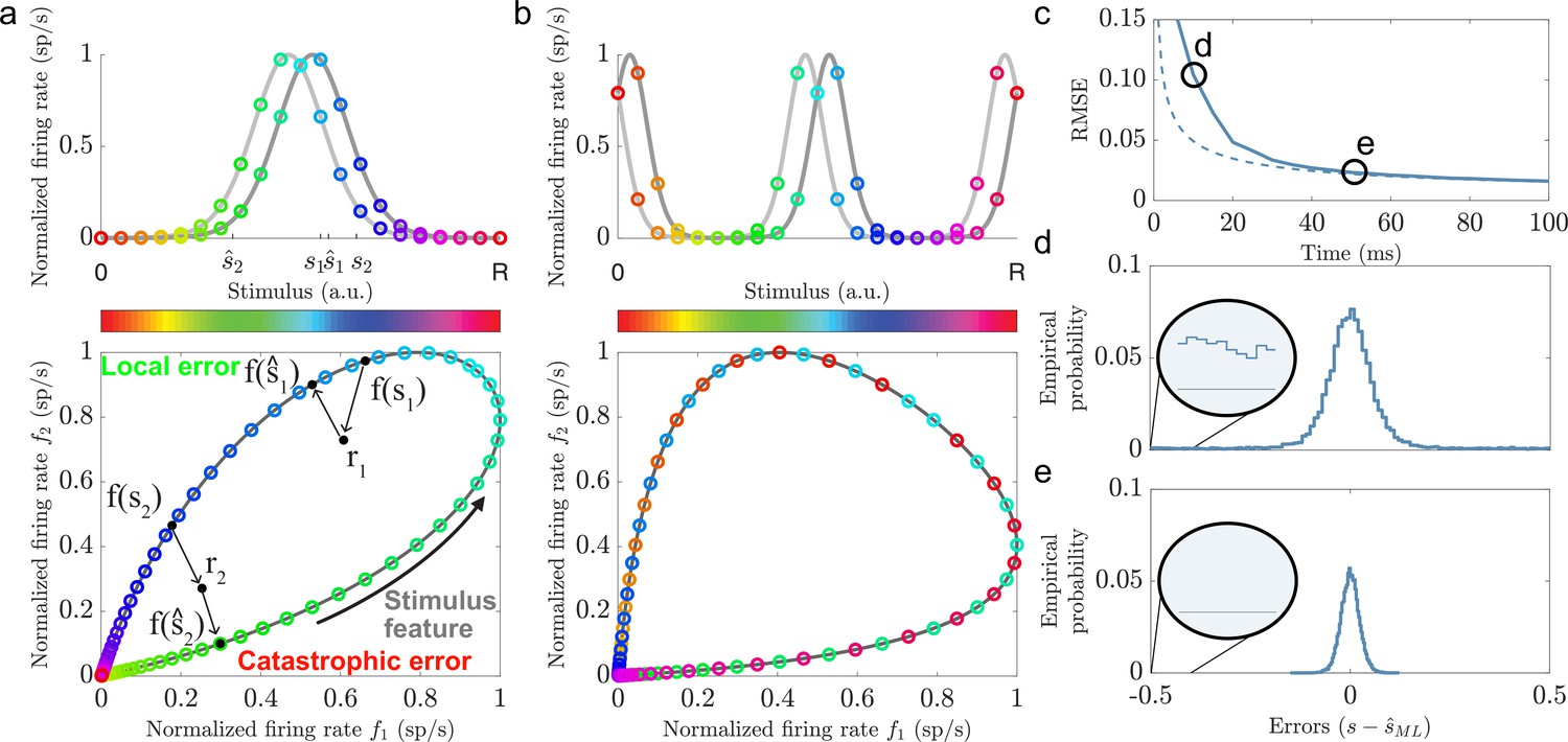
Illustrations of local and catastrophic errors.

(a) Top: A two-neuron system encoding a single variable using single-peaked tuning curves ( $λ = 1$ ). Bottom: The tuning curves create a one-dimensional activity trajectory embedded in a two-dimensional …

Figure 2

Download asset Open asset

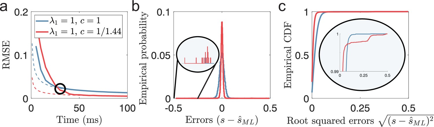
(Very) Short decoding times when both Fisher information and MSE fails.

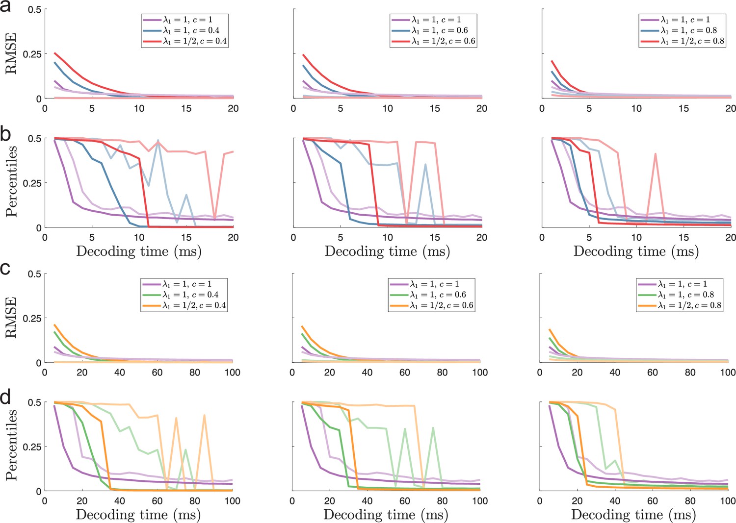
(a) Time evolution of root mean squared error (RMSE), averaged across trials and stimulus dimensions, using maximum likelihood estimation (solid lines) for two populations (blue: $λ_{1} = 1$ , $c = 1$ , red: $λ_{1} = 1$ , $c = 1 / 1.44$ )…

Figure 3 with 2 supplements

Download asset Open asset

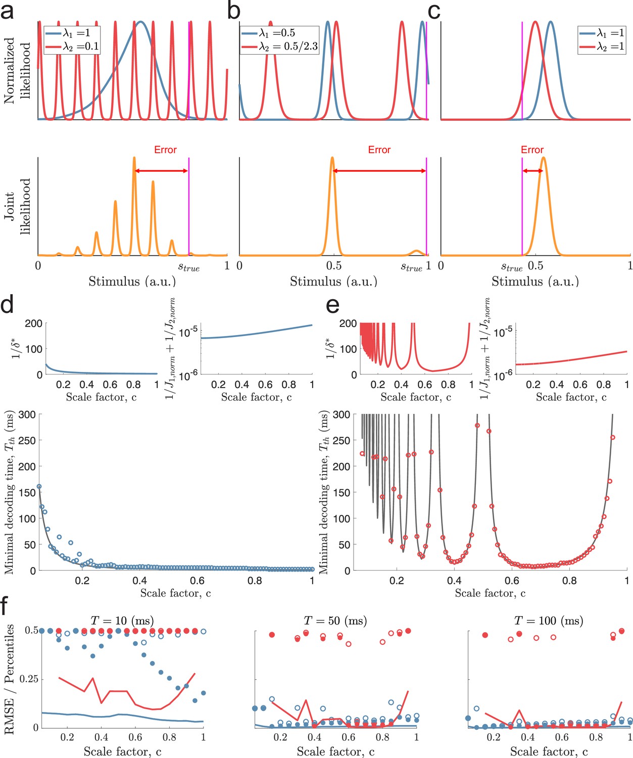
Catastophic errors and minimal decoding times in populations with two modules.

(a) Top: Sampled individual likelihood functions of two modules with very different spatial periods. Bottom: The sampled joint likelihood function for the individual likelihood functions in the top …

Figure 3—figure supplement 1

Download asset Open asset

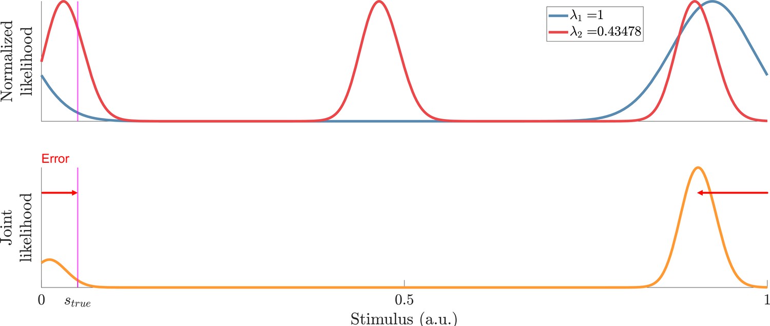
Example of decoding a stimulus close to the periodic edge.

Top: Sampled likelihood functions of two modules with $λ_{1} = 1$ and $λ_{2} = 1 / 2.3$ . Bottom: The joint likelihood function is shifted across the periodic boundary. Such shifts across the periodic boundary can become …

Figure 3—figure supplement 2

Download asset Open asset

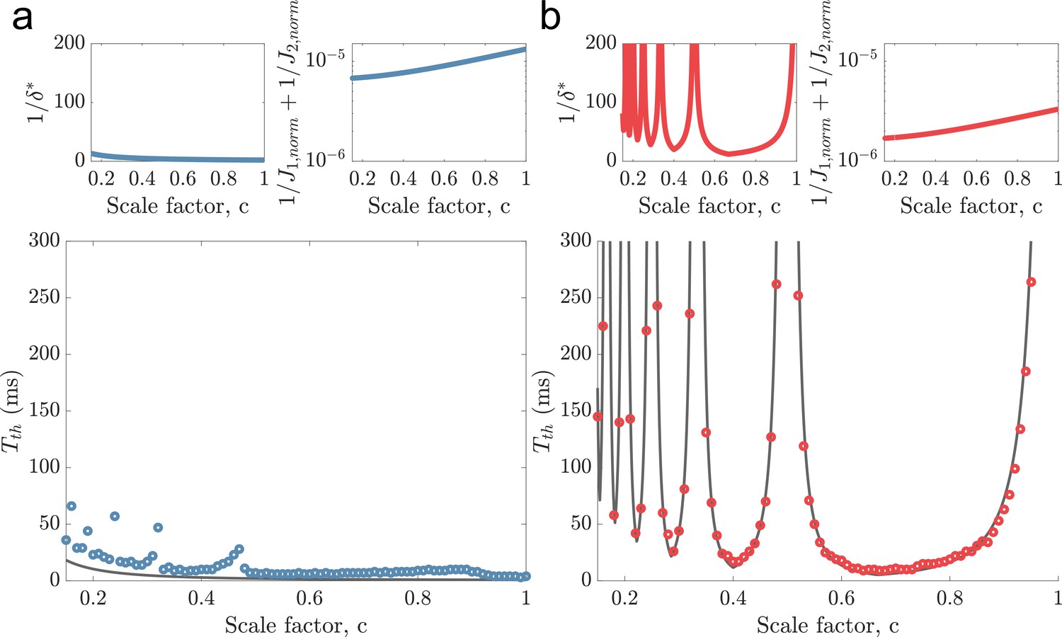
Same as (Figure 2d–e) but using threshold factor $α = 1.2$ .

Notice the stronger deviations from the predicted minimal decoding time for $λ_{1} = 1$ when c is slightly below $1 / 2, 1 / 3, 1 / 4, \dots$ , etc.

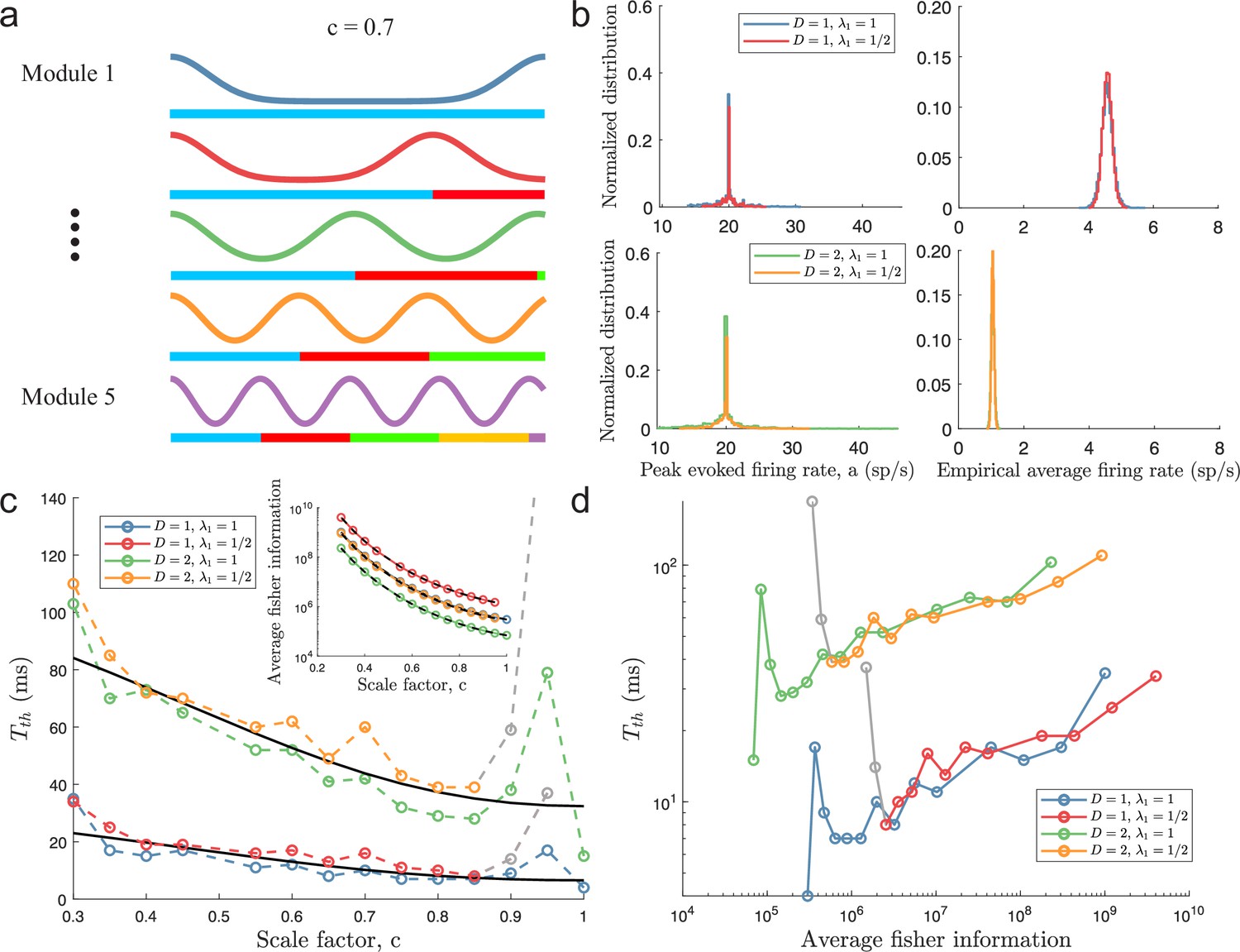
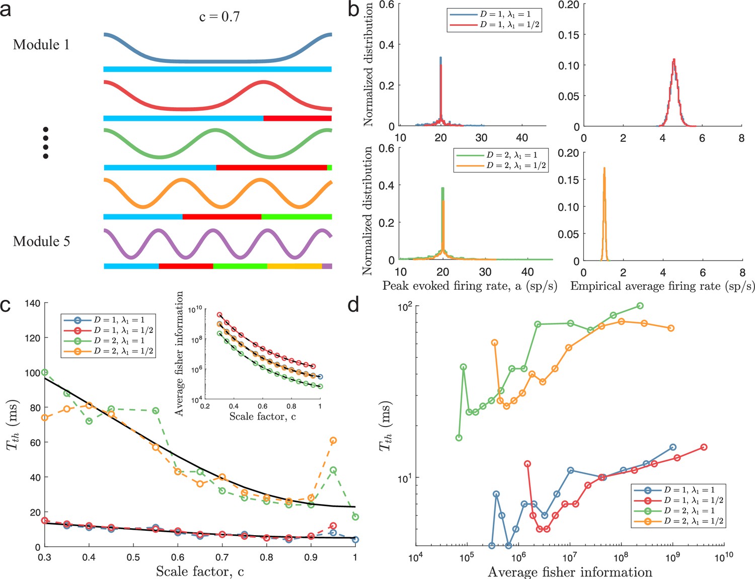
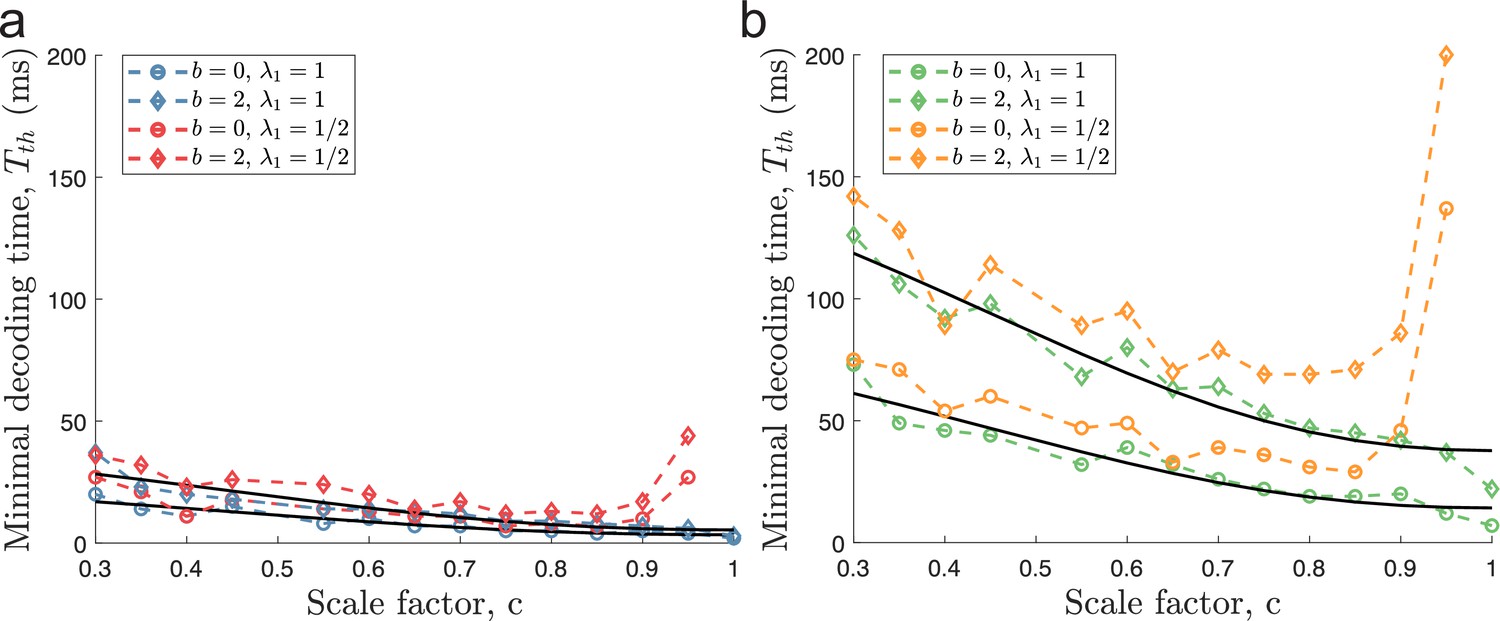
Figure 4 with 6 supplements

Download asset Open asset

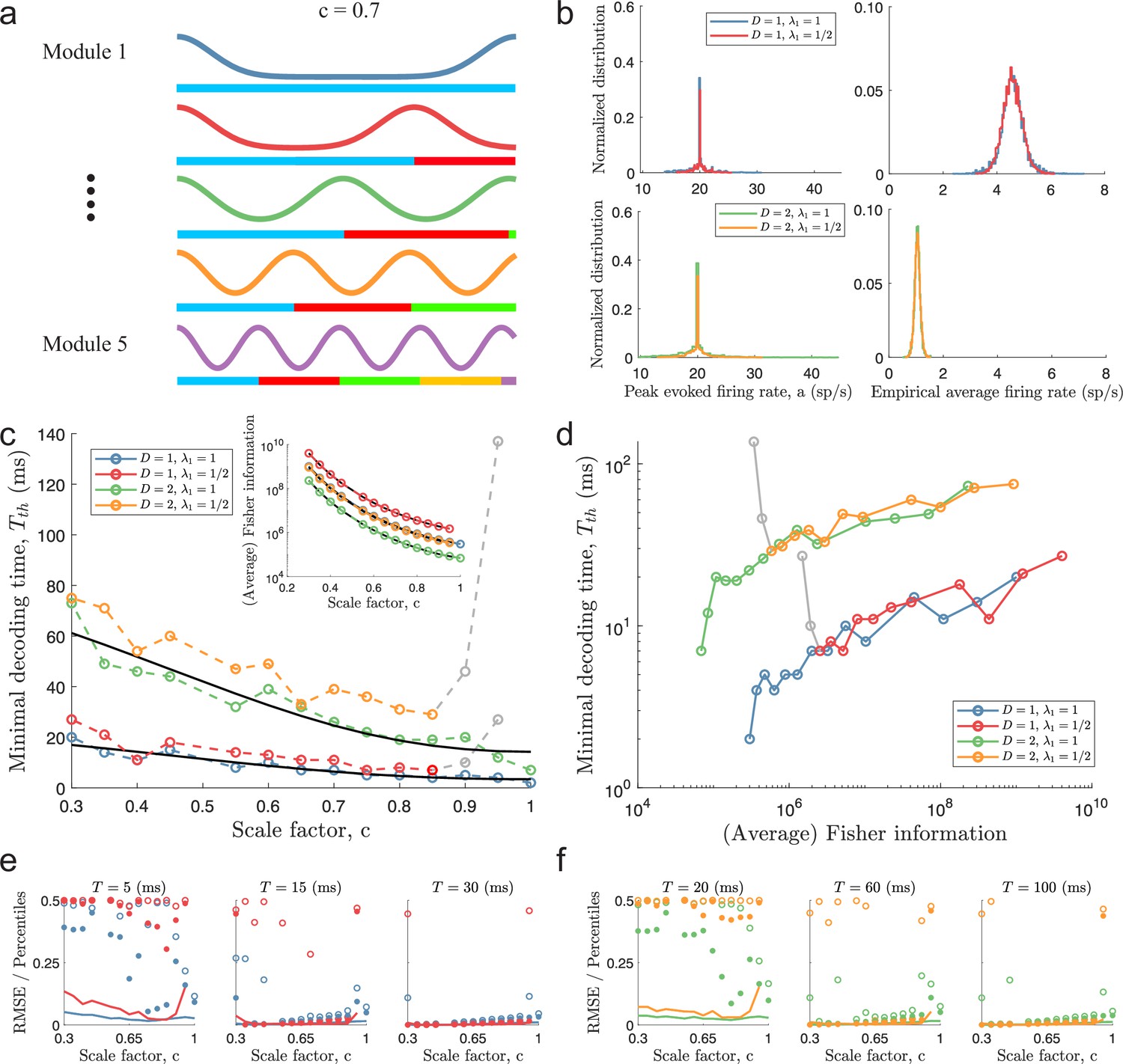
Minimal decoding times for populations with five modules.

(a) Illustration of the likelihood functions of a population with $L = 5$ modules using scale factor $c = 0.7$ . (b) The peak stimulus-evoked amplitudes of each neuron (left column) were selected such that all …

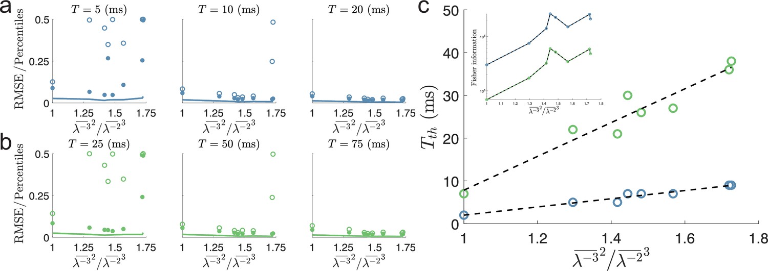
Figure 4—figure supplement 1

Download asset Open asset

Scaling of minimal decoding time with stimulus dimensionality and tuning width.

(a) The predicted minimal decoding time from $D = 1$ scaled by $\frac{\exp (1 / w)}{B_{0} (1 / w)}$ provides a reasonable prediction of the minimal decoding time for $D = 2$ . The data used is the same as in Figure 4c (solid lines with …

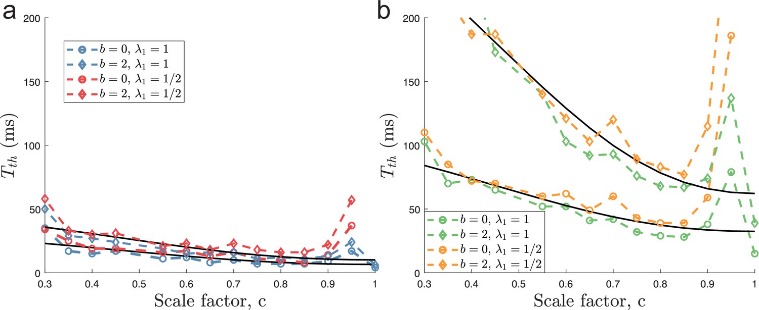
Figure 4—figure supplement 2

Download asset Open asset

Minimal decoding times using a different threshold factor.

Same as Figure 4a–d in the main text, but simulated using threshold factor. For each $T$ , the MSE is evaluated based on 15,000 random stimulus samples.

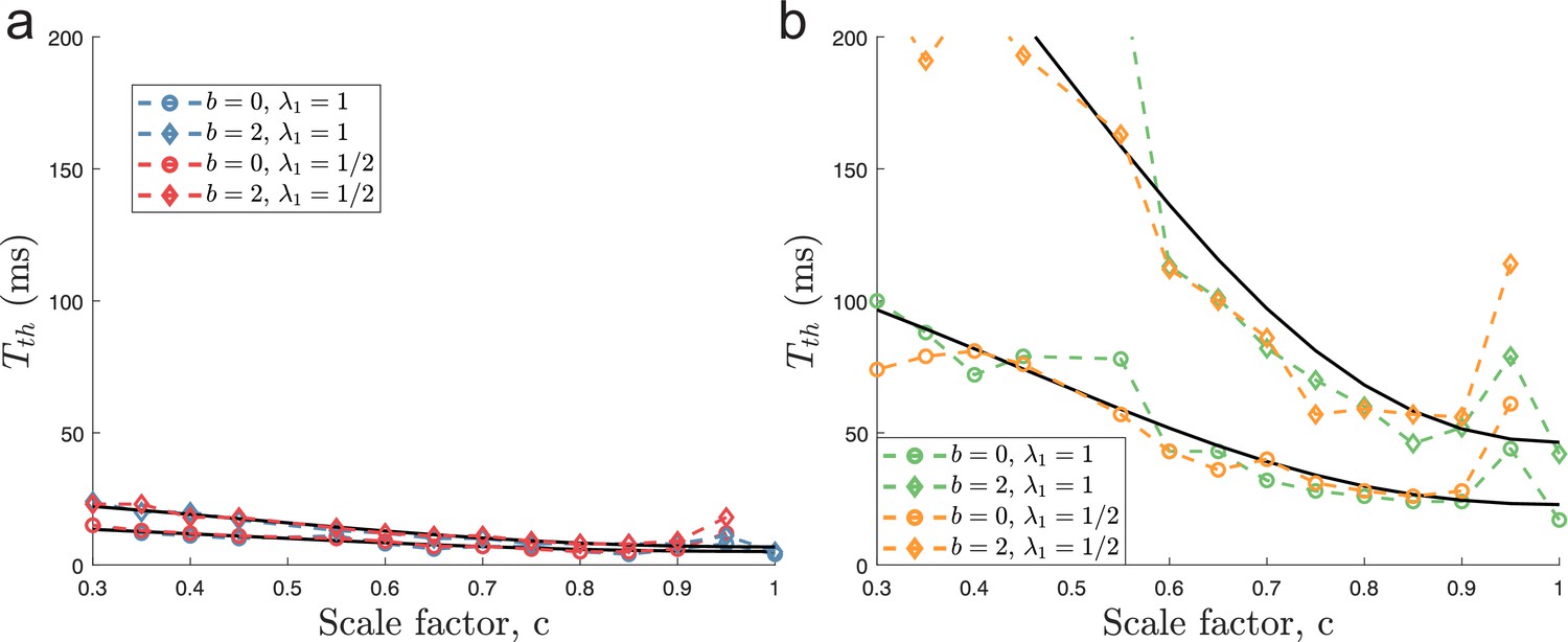
Figure 4—figure supplement 3

Download asset Open asset

Minimal decoding times based on one-sided KS-tests.

Same as Figure 4a–d in the main text, but simulated using the one-sided KS-test for determining minimal decoding time (see main text for details). For each $T$ , the MSE is evaluated based on 15,000 …

Figure 4—figure supplement 4

Download asset Open asset

Time evolution of MSE and outlier errors.

(a) Time evolution of the RMSE (non-transparent lines) for periodic and single-peaked populations and the lower bound set by the Cramér-Rao bound (transparent lines) when decoding a $D = 1$ stimulus. (b) …

Figure 4—figure supplement 5

Download asset Open asset

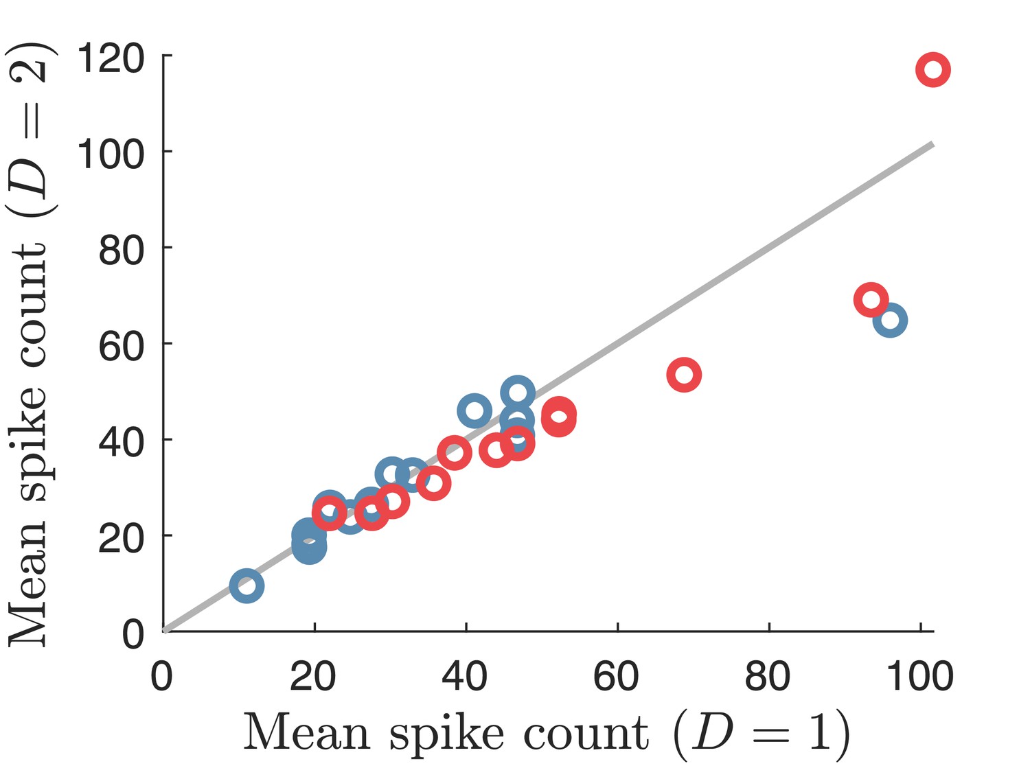
Spike counts required for removing catastrophic errors.

Plot of the mean spike counts (summed over the population) required to remove catastrophic errors for the populations in Figure 4. Each circle indicates the minimal spike count for a single …

Figure 4—figure supplement 6

Download asset Open asset

Minimal decoding times for populations without scale factors.

Same as Figure 4c, e and f, but only using tuning curves with an integer number of peaks, that is, being all integers. Thus, there is no common scale factor relating the spatial frequencies of the …

Figure 5

Download asset Open asset

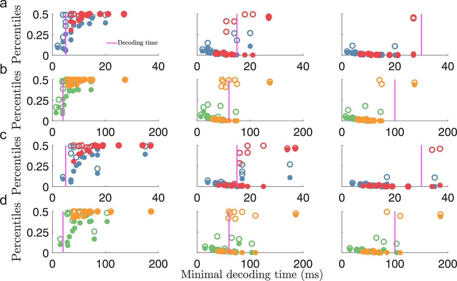
Minimal decoding time predicts the removal of large estimation errors.

(a) The 99.8th percentile (filled circles) and the maximal error (i.e., 100th percentile, open circles) of the root squared error distributions for $D = 1$ against the estimated minimal decoding time for …

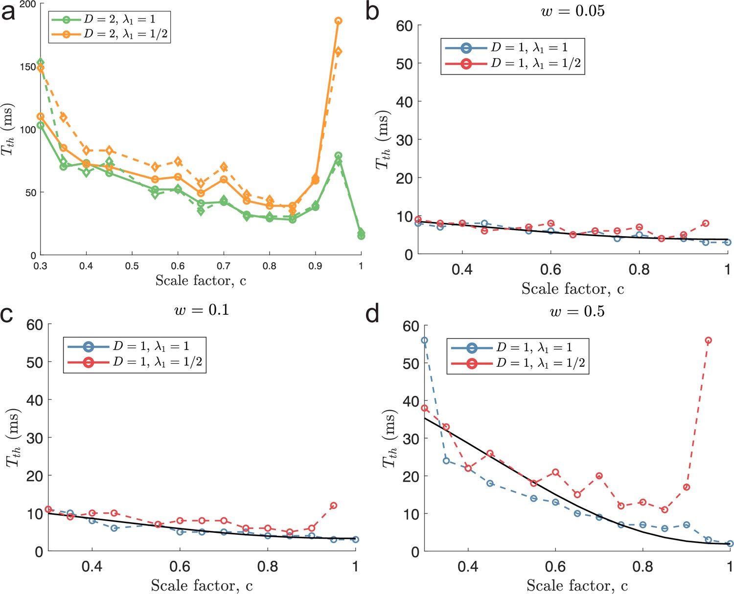
Figure 6 with 2 supplements

Download asset Open asset

Ongoing activity increases minimal decoding time.

(a) The case of encoding a one-dimensional stimulus ( $D = 1$ ) with or without ongoing activity at 2 sp/s (diamond and circle shapes, respectively). (b) The case of a two-dimensional stimulus ( $D = 2$ ) under …

Figure 6—figure supplement 1

Download asset Open asset

Minimal decoding times using a different threshold factor.

Same as Figure 6 in the main text, but using $α = 1.2$ .

Figure 6—figure supplement 2

Download asset Open asset

Minimal decoding times based on one-sided KS-test.

Same as Figure 6 in the main text, but using the one-sided KS-test criterion described before (see Figure 4—figure supplement 4).

Figure 7

Download asset Open asset

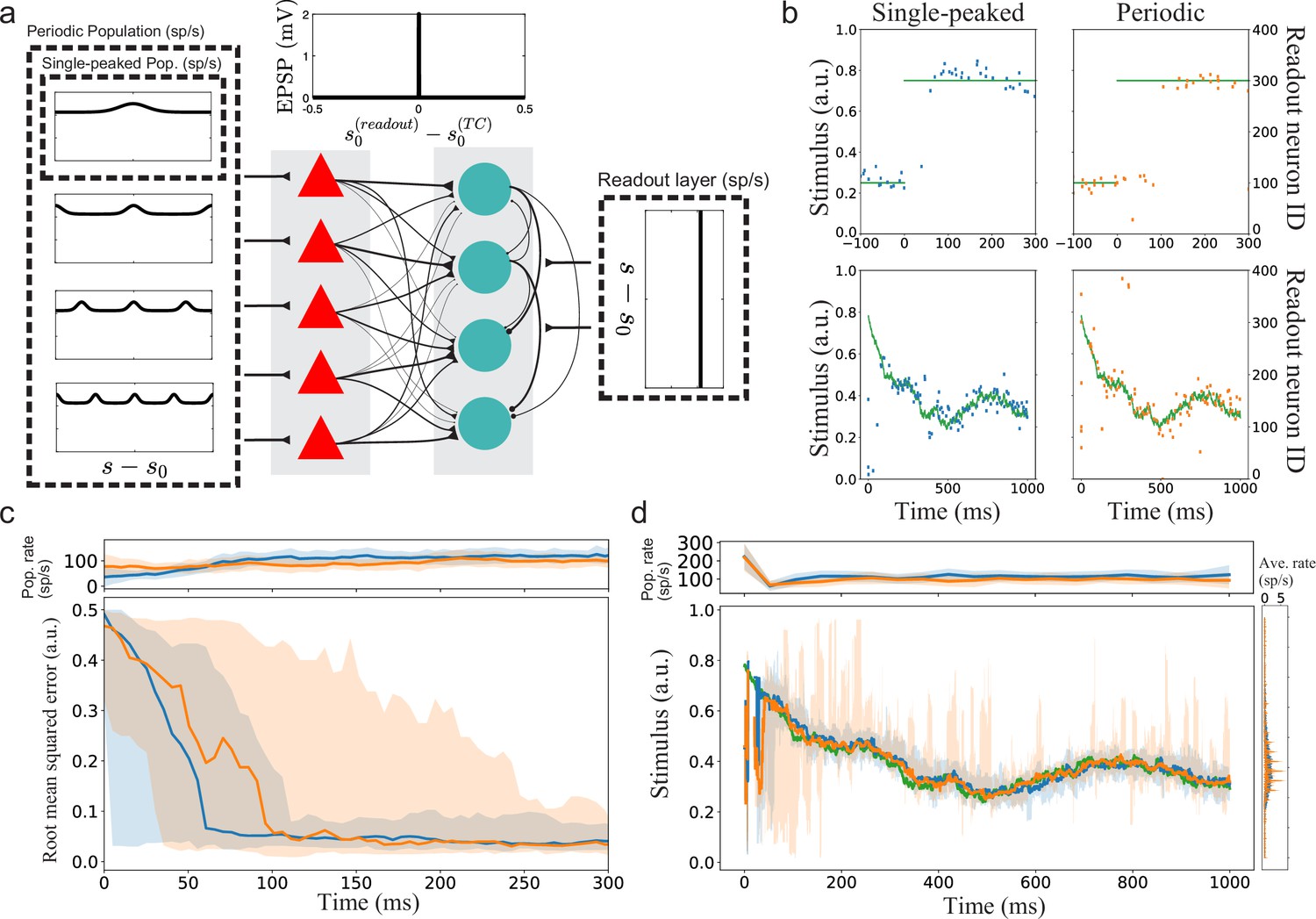
Implications for a simple spiking neural network with suboptimal readout.

(a) Illustration of the spiking neural networks (SNNs). (b) Example of single trials. Top row: Two example trials for step-like change in stimulus (green line). The left and right plots show the …

Figure 8

Download asset Open asset

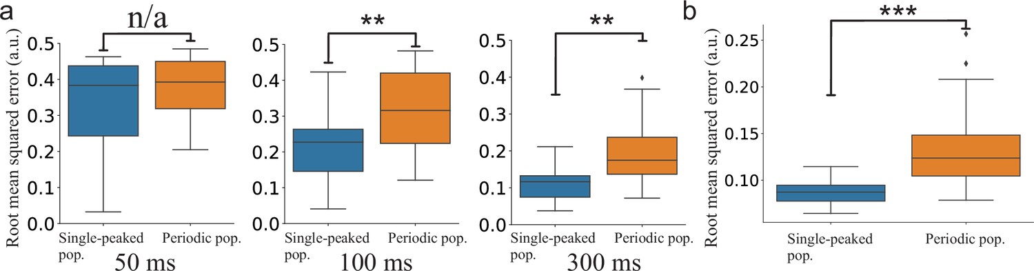
Statistical comparison of the SNN models.

(a) Step-like change: Comparison between the distributions of accumulated RMSEs at different decoding times ( $p = 0.4$ , $9.0 \cdot 10^{- 4}$ , and $8.7 \cdot 10^{- 5}$ , respectively). (b) OU-stimulus: The distributions of RMSE across trials …

Figure 9

Download asset Open asset

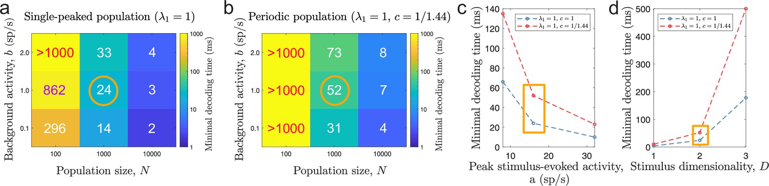
Minimal decoding time for various tuning and stimulus parameters.

(**a-b**) Minimal decoding time for different combinations of population sizes ( $N$ ) and levels of ongoing background activity ( $b$ ) for the single-peaked population (a) and the periodic population (b). (c…

Tables

Table 1

Parameters and parameter values for O-U stimulus.

Parameters	Parameter values
$τ_{s}$	0.5 (s)
$σ_{s}$	0.1

Table 2

Parameters and parameter values for LIF neurons.

Parameters	Parameter values
Membrane time constant, $τ_{m e m b}$ (ms)	20
Threshold memb. potential, $V_{t h}$ (mV)	20
Reset memb. potential (mV)	10
Resting potential, V₀ (mV)	0
Refractory period, $τ_{r p}$ (ms)	2

Table 3

Spiking network parameters and parameter values.

Parameters	Parameter values
Number of neurons 1st layer, N₁	500
Number of neurons 2nd layer, N₂	400
Maximal stimulus-evoked input rate, $a$ (sp/s)	750
Baseline input rate, $b$ (sp/s)	4250
Spatial periods, $λ_{j}$	[1] or [1,2,3,4]
Width parameter, $w$	0.3
Width parameter (readout layer), $w_{r o}$	$\frac{(π / N_{2})^{2}}{2 \log (2)}$
Input EPSP (1st layer), $J_{E}$ (mV)	0.2
Maximal EPSP (2nd layer), $J_{E E}$ (mV)	2
Maximal IPSP (2nd layer), $J_{I I}$ (mV)	2
Synaptic delays, $d$ (ms)	1.5